Modeling the Effects of Anthropogenic Land Cover Changes to the Main Hydrometeorological Factors in a Regional Watershed, Central Greece

Abstract

In this study, the physically-based hydrological model MIKE SHE was employed to investigate the effects of anthropogenic land cover changes to the hydrological cycle components of a regional watershed in Central Greece. Three case studies based on the land cover of the years 1960, 1990, and 2018 were examined. Copernicus Climate Change Service E-OBS gridded meteorological data for 45 hydrological years were used as forcing for the model. Evaluation against observational data yielded sufficient quality for daily air temperature and precipitation. Simulation results demonstrated that the climatic variabilities primarily in precipitation and secondarily in air temperature affected basin-averaged annual actual evapotranspiration and average annual river discharge. Nevertheless, land cover effects can locally outflank the impact of climatic variability as indicated by the low interannual variabilities of differences in annual actual evapotranspiration among case studies. The transition from forest to pastures or agricultural land reduced annual actual evapotranspiration and increased average annual river discharge while intensifying the vulnerability to hydrometeorological-related hazards such as droughts or floods. Hence, the quantitative assessment of land cover effects presented in this study can contribute to the design and implementation of successful land cover and climate change mitigation and adaptation policies.

1. Introduction

The quantitative and qualitative state of water resources of a watershed are formed by a variety of drivers that interact in a complex and often indirect way [1]. Climate elements (precipitation; relative humidity; wind speed and direction; solar radiation and temperature that also controls evaporation/evapotranspiration and snow melt and their temporal and spatial distribution) and the biogeophysical characteristics of a catchment (topography, land—vegetation cover, geological structure, soil coverage) are fundamental determinants of regional hydrology [2,3]. The conceptual model describing the interactions among the abovementioned drivers is the hydrological cycle that links the exchange, storage and movement of water among the biosphere, atmosphere, cryosphere, lithosphere, anthroposphere, and hydrosphere [4], while the quantification of the relationships among the components of the hydrological cycle at a given location constitutes the water balance [5].

All characteristics of the catchment (climate elements and biogeophysical characteristics) are factors that can be largely affected by anthropogenic activities and pressures [3]. Humanly imposed climate change due to increased emissions of greenhouse gases and dust from anthropogenically-disturbed soils [6], is expected to significantly increase freshwater-related risks such as modification of the hydrological regime, floods and droughts, and to affect water cycle components [7,8]. Climate change is projected to reduce renewable surface water and groundwater resources significantly in most dry subtropical regions and is likely to increase the frequency of meteorological droughts (less rainfall) and agricultural droughts (less soil moisture) in presently dry regions. Additionally, projections imply variations in the frequency of floods and negative impacts on freshwater ecosystems by changing streamflow and water quality [4,7]. Regarding anthropogenic interventions in catchment’s physical characteristics (for example alteration of the land surface soil moisture, albedo and roughness [9]), land cover changes due to livestock grazing, agriculture, timber harvest, deforestation, and urbanization can reduce retention of water in watersheds and lead to an increase of the size and frequency of floods and to the reduction of baseflow levels [10]. Dam constructions and diversion, canalization, snagging and dredging of rivers, streams and drainage ditches, and groundwater overexploitation, disrupt the dynamic equilibrium between the movement of water and sediment that exists in rivers [10]. Based on recent studies, direct human impacts on the terrestrial water cycle are in some large river basins of the same order of magnitude, or even larger than climate change [11,12]. Especially land cover change alters annual global runoff to a similar or greater extent than other major drivers [13], while land use change contribution in regional runoff values in tropical regions is larger than that of climate change [14], especially in the case of smaller catchments [15].

Worldwide studies support the impacts of land cover changes, mainly deforestation and urbanization, on the hydrometeorological factors, leading primary to river discharge increase [16,17,18,19,20,21,22,23] and generally to an increase of eco-environmental vulnerability of the watersheds [24,25]. In Greece, studies confirm the impact of land cover change and deforestation in river discharge. For example, a study conducted in Pinios river basin proved that expanding the agricultural land over forest by 20%, a mean monthly increase in the river discharge of up to 3%, can be observed from October to April and a respective reduction from May to September, reaching a maximum of 6% in July [26]. Moreover, human interference in streams crossing urban or suburban areas raise the vulnerability to flash floods. For example, the hydrometeorological analysis of a fatal flash flood event which occurred on 15 November 2017 in the suburban area of Mandra, western Attica, Greece resulting in extensive damages and 24 fatalities, showcased heavy storm-induced run-off water in combination with human pressures on streams as the reason for the flood [27].

Regarding the impact of land cover change to evapotranspiration, it has been reported that mean annual evapotranspiration can be up to 39% lower in agricultural ecosystems than in natural ecosystems in Brazil [20]. A recent study concerning the whole of China showed that the average annual land surface evapotranspiration decreased at a rate of −0.6 mm/yr from 2001 to 2013, attributed partly to land use and land cover changes of forests to other land types [28]. In Greece, a study in a small catchment showed that 16% increase of agricultural land against wetland and forest area led to a 6% increase of evapotranspiration and 10% increase of the water deficit in the soil [29].

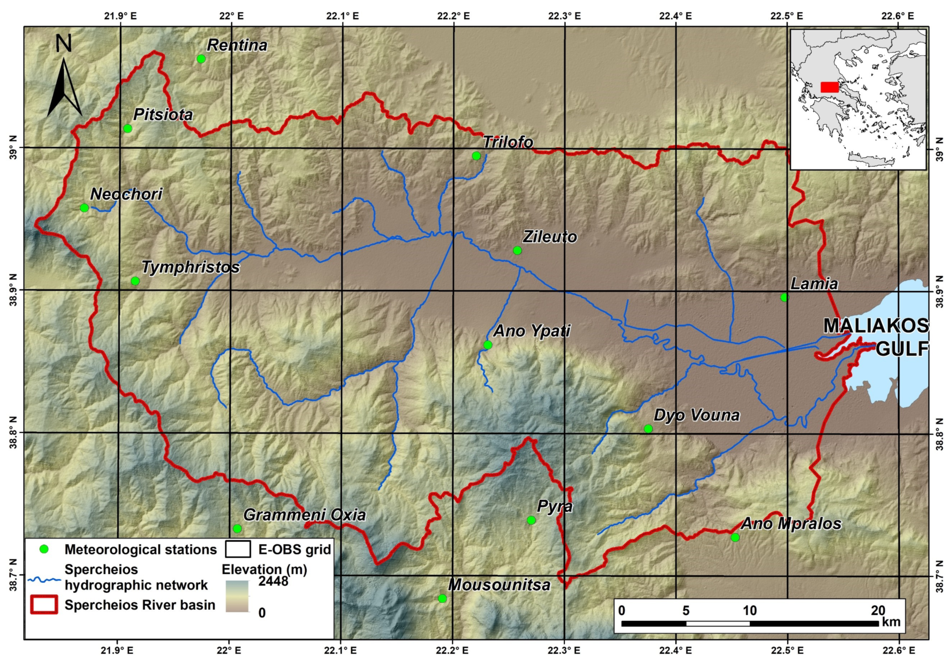
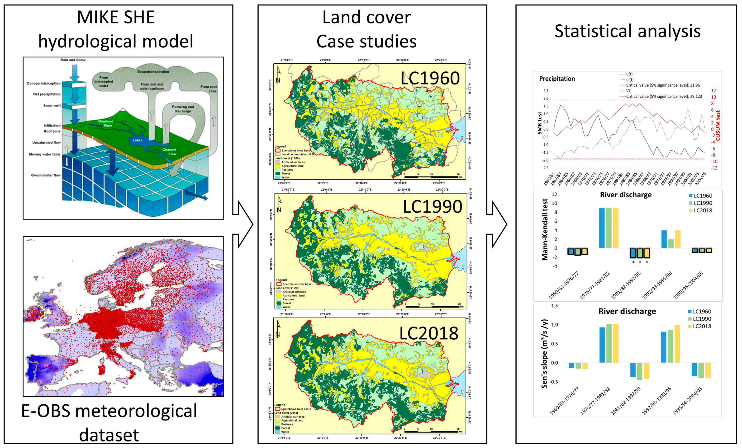
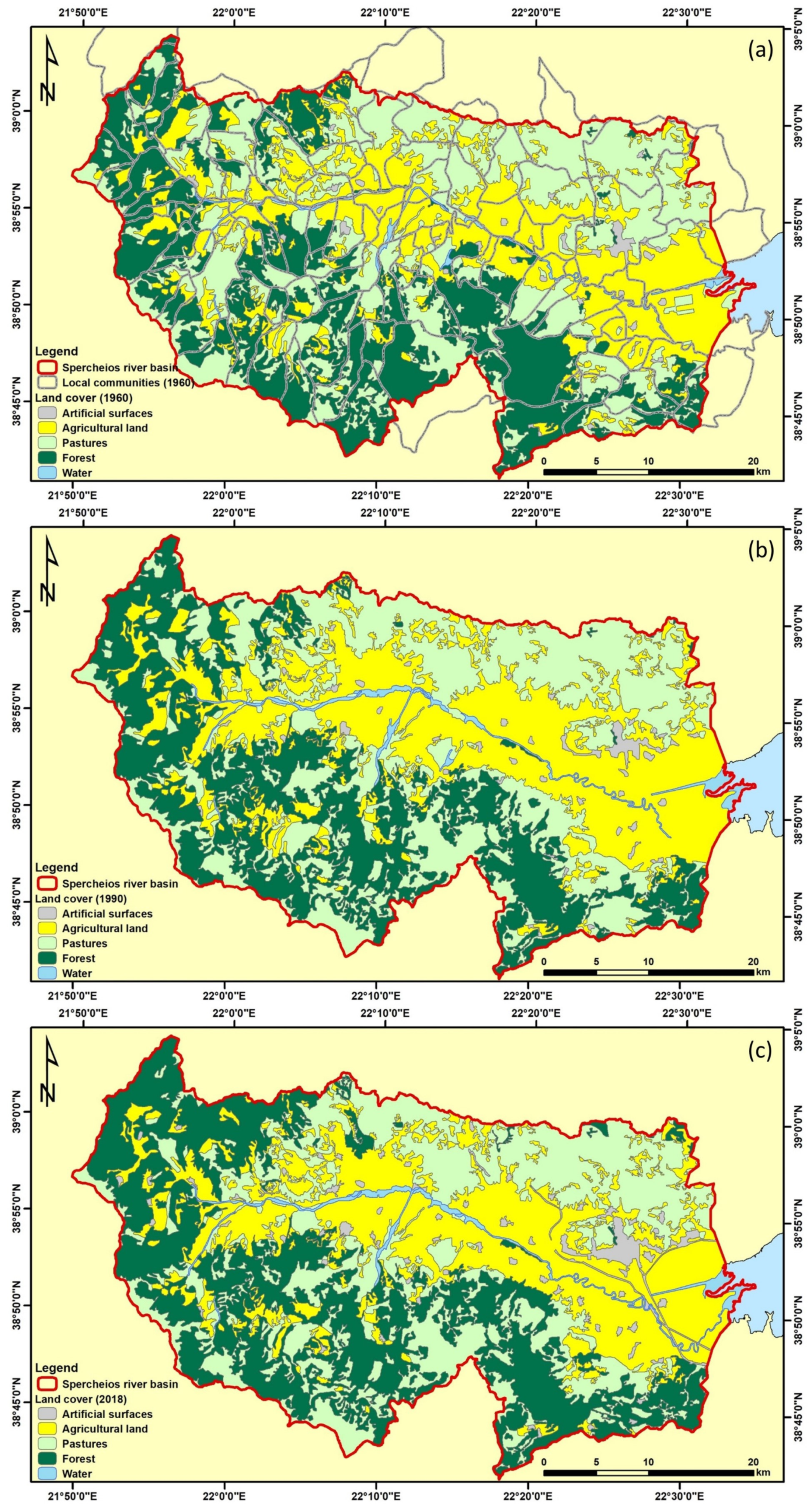
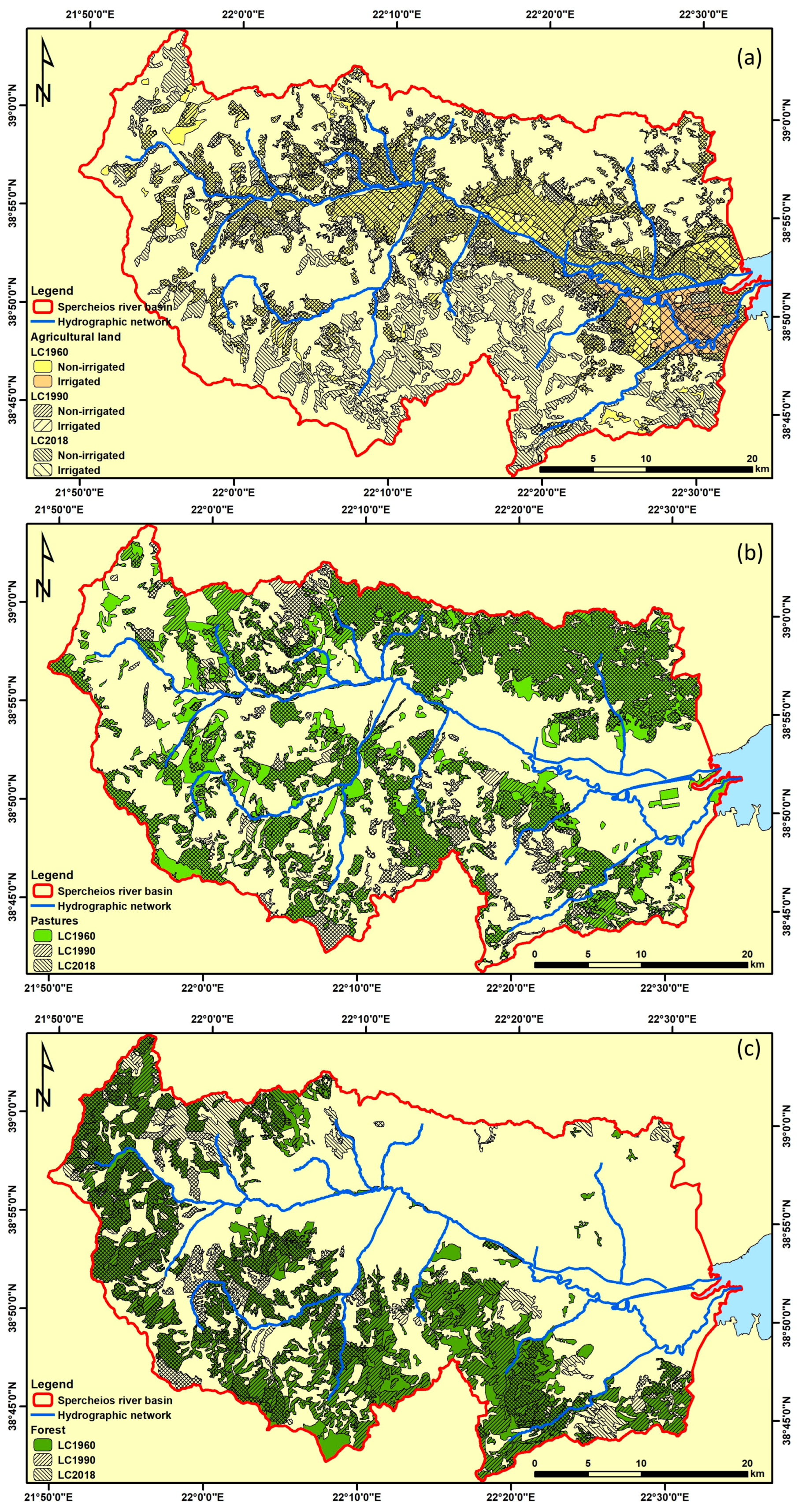
Given the uncertainty of future land cover changes due to socio-economic driving forces and local development policies applied, a scenario-based modeling framework can be beneficial in supporting the analysis of potential land cover changes, so as to mitigate potentially negative future impacts on a basin’s water resources. In order to investigate the effect of anthropogenic land cover changes to the hydrological cycle components and the main hydrometeorological factors of a regional agricultural watershed in Central Greece (Spercheios river basin) of great ecological value, three (3) land cover case studies were adopted, based on the land cover distribution documented in the following years: in 1960 (hereafter LC1960; baseline), in 1990 (hereafter LC1990; mid-period), and in 2018 (hereafter LC2018; current state). The modeling tool used was the physically-based hydrological model (MIKE SHE), while the high-resolution gridded observational daily meteorological dataset of Europe named E-OBS [27] from the EU-FP6 project UERRA [30] and the Copernicus Climate Change Service [31] was also employed to drive the model. Since the E-OBS gridded dataset had not been used before in similar studies in Greece, the statistical evaluation of its efficiency was considered to be obligatory before performing any further analysis. Finally, statistical tests and trend analysis were performed on the simulated time series of each land cover case study examined.

The main objective of the present study was the better understanding of the system’s response and the basin’s water resources to possible future land cover changes, while the main research questions intended to be addressed are: (a) which are the interrelationships among land cover and the main hydrometeorological factors’ (precipitation, air temperature, discharge, and actual evapotranspiration) variations, (b) how land cover changes affect the trend magnitude of the main hydrometeorological factors, and (c) which are the hydrometeorological-related hazards associated with land cover changes in the study area?

2. Materials and Methods

2.1. Study Area

Spercheios river basin is located in the prefecture of Pthiotida in Central Greece, covers an area of 1,661 km², and has a mean altitude of 641 m and a dense hydrographic network (Figure 1; [32]). The main human activities of the wider area since it was first inhabited in the Early Neolithic period [33] include arable agriculture and grazing, while industrial activities are limited mainly to small manufacturing units of agricultural products and olive oil refineries [34]. The main hydromorphological modifications of the area include water abstractions for irrigation, water flow regulations (small weirs, water distributor), canalization, and the partial diversion of the original route of the river close to its estuary. Spercheios river wider area has been included in many environmental protection networks (for example NATURA 2000, CORINE biotopes, and Wildlife Refuges; [32,35]).

2.2. Hydrological Simulation

2.2.1. Methodological Approach

The modelling tool used in the present study was the MIKE SHE, developed by the Danish Hydraulic Institute Water and Environment. MIKE SHE is a physically-based distributed model that is able to simulate all hydrological domains within the land phase of the hydrological cycle in a river basin. MIKE SHE is fully integrated with the channel flow code MIKE 11, which is a one-dimensional model that can simulate water flow and level, water quality and sediment transport in rivers, flood plains, irrigation canals, reservoirs, and other inland water bodies [36]. The hydrological model has already been successfully set up, calibrated and validated during a previous study for Spercheios river basin [35].

More specifically, during a previous research study, the hydrological model of Spercheios river basin was set up and calibrated for the hydrological years 2008/2009–2010/2011 and validated for the hydrological years 2013/2014–2014/2015 [35]. These periods were chosen based on the data availability (actual in situ observations of water level and discharge and high-quality climatological data) and on the fact that in 2008 the construction of the last engineering flood control structures in the hydrological network and the river banks were completed. The calibration and validation periods’ length were considered to be adequate since most studies addressing the question of the utility of additional data in terms of the length of available discharge time-series in hydrological model calibration concluded that several years of data ranging between 2 and 8 years are sufficient for reliable parameter identification [37]. Moreover, when 2–3 years of continuous daily discharge data are available, then the model activates the complete set of its procedures, and the use of longer data sets would not offer a significant benefit in the definition of the model’s uncertainty [38]. The results of the Spercheios river basin hydrological model calibration showed a satisfactory agreement between observed and simulated water levels and discharge measurements. Their correlation coefficient R can be characterized as moderate (0.55) to high (0.77) based on the criteria for correlation interpretation proposed by Hinkle et al. [39], and in all cases the data were statistically significant at the 0.05 level, indicating the sufficient performance of the model. During validation, the resulted correlation coefficient R was also moderate (0.68) to high (0.84) [39], and the data were also statistically significant at the 0.05 level. The model performance can be considered satisfactory since the results meet the criteria proposed by Moriasi [40] (R2 > 0.50, RSR < 0.70, and PBIAS ± 25% for streamflow) in the cases where river discharge data were available for validation [35] (

Table 1. Statistical characteristics and efficiency criteria for the calibration and validation of the hydrological model at the Spercheios river basin [35].

Station		Para-Meter	Statistical Parameter
			N	ME	MAE	RMSE	R	p-Value	R2	PBIAS	RSR
Kastri bridge	Calibration	L	1095	0.065	0.177	0.238	0.77	<0.00001 *	0.56	-	-
Kompotades bridge		L	909	0.042	0.273	0.387	0.55	<0.00001 *	0.11	-	-
Komma bridge		L	1063	−0.105	0.351	0.479	0.61	<0.00001 *	0.34	-	-
KR2	Validation	L	176	0.063	0.102	0.138	0.70	<0.00001 *	-1.06	-	-
KR3		L	236	0.009	0.085	0.143	0.80	<0.00001 *	0.62	-	-
KR6		L	303	0.146	0.266	0.366	0.68	<0.00001 *	-1.24	-	-
KR7		L	462	−0.060	0.195	0.405	0.76	<0.00001 *	−0.88	-	-
KR2		Q	12	0.735	1.164	1.777	0.79	0.002333 *	0.48	32%	0.21
KR3		Q	11	−0.718	1.304	2.007	0.84	0.001277 *	0.56	−27%	0.20

* result significant at p < 0.05; L: Level (m); Q: Discharge (m³/s); N: number of sample pairs; ME: mean error; MAE: mean absolute error; RMSE: root mean squared error; R: correlation coefficient; R2: Nash-Sutcliffe coefficient of efficiency; PBIAS: percent bias; RSR: RMSE-observations standard deviation ratio.

).

In order to investigate the impact of land cover change on the hydrological cycle components, the calibrated hydrological model of Spercheios river basin was integrated for 45 hydrological years (1960/61–2004/05) for three different land cover case studies. The specific period was characterized by a stable hydrographic network with minimum engineering interventions. Any hydraulic construction built after 2006 was omitted from simulation procedure, while all engineering interventions which took place before 1960 were included into the simulation, for the best representation of the actual state of the river network during the period 1960/61–2004/05. For the specific simulation period, the gridded time-series of the meteorological dataset used for the specific study area was complete and without gaps. Finally, the land cover case studies were selected according to the data availability and taking into consideration the overall anthropogenic interventions in the area, aiming at the better representation of each distinguished period. More specifically, until 1960, the major hydraulic interventions and the major agricultural reform of Greece had been completed, and ever since the area used for agricultural activities has been practically stable in the study area [41]. The first available documentation concerning the land cover distribution in Greece was from the year 1960 [42]. In 1990, the first pan-European land cover data collection was utilized based on satellite image processing (Coordination of Information on the Environment- CORINE Land Cover Programme [43]), and the most recent version is from the year 2018 [44]. Therefore, the following three land cover case studies in Spercheios river basin were implemented: (1) LC1960 based on the land cover of Spercheios river basin in 1960 (baseline), (2) LC1990 based on the land cover in 1990 (mid-period) and (3) LC2018 based on the land cover in 2018 (current state) (Figure 2).

2.2.2. Meteorological Data

Due to the lack of detailed and evenly distributed meteorological time-series in Spercheios river basin covering the entire simulated period (1960/61–2004/05), the necessary data for the hydrological modeling concerning daily temperature (minimum, average and maximum values) and precipitation were retrieved from the high-resolution gridded data set of daily climate over Europe termed E-OBS from Copernicus Climate Change Service [45,46]. The specific data set covers the period back to 1950 and provides high-resolution gridded fields at a spacing of 0.1° × 0.1° in regular latitude/longitude coordinates. The ensemble version of E-OBS v.19.0e (the dataset produced from averaging multiple equally probable interpolations of station-based observations, so as to provide the best representation of the spatial and temporal distribution of climate parameters and a measure of uncertainty [47]) is based on the European Climate Assessment and Dataset (ECA&D) initiative that combines collation of daily series of observations at meteorological stations, quality control, analysis of extremes, and dissemination of both the daily data and the analysis results (Figure 1; [48,49]).

The reliability of the E-OBS dataset was evaluated by comparing the time-series of in-situ observations from meteorological stations installed in the wider area by various agencies (

Table 2. Meteorological stations used in estimation of E-OBS efficiency.

Station	Longitude (dd)	Latitude (dd)	Altitude (m)	Owner	Observations Available
Ano_Mpralos	22.45474	38.73054	580.5	MEE	P
Ano_Ypati	22.23273	38.86562	286.0	MEE	P
Dyo Vouna	22.37684	38.80680	470.6	PPC	P
Gr. Oxia	22.00846	38.73601	1107.1	PPC	P, Tmin, Tmax
Lamia	22.49940	38.89895	144.0	HNMS	P, Tmin, Tmax, Tav
Mousounitsa	22.19244	38.68742	846.1	MEE	P, Tmin, Tmax
Neochori	21.86983	38.96068	821.6	PPC	P
Pitsiota	21.90836	39.01663	783.9	PPC	P
Pyra	22.27196	38.74262	1137.1	MEE	P
Rentina	21.97414	39.06577	884.9	MEE	P
Trilofo	22.22209	38.99834	575.3	MEE	P
Tymphristos	21.91575	38.90961	847.9	MEE	P
Zileuto	22.25904	38.93192	97.2	MEE	P

MEE: Ministry of Environment and Energy of Greece; HNMS: Hellenic National Meteorological Service; PPC: Public Power Corporation S.A.; P: precipitation; Tmin: minimum air temperature; Tmax: maximum air temperature; Tav: mean air temperature.

; Figure 1) against the corresponding grid point of the E-OBS dataset. The statistical criteria used to investigate the dataset reliability were the following: mean error ME; mean absolute error MAE; root mean squared error RMSE; standard deviation STDEV; and correlation coefficient R, while also the p-value was calculated to estimate the significance of the results.

The lack of the necessary climatological data (relative humidity, solar radiation and wind speed) precluded the use of the Penman-Monteith equation for the estimation of daily reference evapotranspiration ET. Therefore, ET was estimated using the Hargreaves empirical approach [50], which is recommended only in cases of lack of other meteorological data and is considered to provide satisfactory results with an error rate of 10–15% or 1 mm/d, whichever is greater [51,52]. In the Hargreaves approach, except for daily average, minimum and maximum temperature, all the other required parameters (solar radiation, latent heat of vaporization) can be estimated using empirical relationships [52].

2.2.3. Land Cover Spatial Distribution

The oldest official and most detailed information concerning land cover distribution in Spercheios river basin was available from National Statistical Service of Greece for the year 1960. These data were part of the preparatory activities taken place prior the Agricultural and Livestock Census of March 19, 1961 [42] and concerned the main land cover types per local community: agricultural land, communal or private pastures for grazing animals, forest, artificial surfaces and water. It should be noted that in the 1960s land cover census, all agricultural activities (annual, crops, vineyards, tree plantations, and fallow land) were grouped together, while areas covered by shrubs, transitional woodland—shrub areas or areas with dense vegetation were characterized as pastures. During this procedure, forests were defined as areas mainly covered by ligneous plants clearly supported by a trunk and branching out to no less than 1 m from the ground. The category artificial surfaces included cities, settlements, roads, mines, and bare rocks. Finally, the category water included lakes, permanent inland and salt marshes, coastal areas and lagoons, estuaries, water courses, river beds, and areas covered by water for the greatest part of the year. Areas temporarily covered by water and areas lying near rivers or lakes dried and usually cultivated in summer were included in arable land (

Table 3. Land cover nomenclature used in the present study.

Level 1	Level 2	1960	1990	2018
Artificial surfaces	Continuous urban fabric	x	x	x
	Discontinuous urban fabric	x	x	x
	Airports		x	x
	Bare rocks		x
	Industrial or commercial units		x	x
	Mineral extraction sites		x	x
	Construction sites			x
	Road and rail networks and associated land			x
	Sport and leisure facilities			x
Agricultural land	Non-irrigated arable land	x	x	x
	Permanently irrigated land	x	x	x
	Complex cultivation patterns	x	x	x
	Land principally occupied by agriculture	x	x	x
	Rice fields	x	x	x
	Olive groves	x	x	x
	Vineyards	x	x
	Fruit trees and berry plantations			x
Pastures	Natural grasslands	x	x	x
	Sclerophyllous vegetation	x	x	x
	Transitional woodland-shrub	x	x	x
	Pastures	x	x	x
	Moors and heathland		x	x
	Sparsely vegetated areas		x	x
Forest	Broad-leaved forest	x	x	x
	Coniferous forest	x	x	x
	Mixed forest	x	x	x
Water	Sea and ocean		x	x
	Estuaries		x	x
	Beaches, dunes, sands		x	x
	Salt marshes	x	x	x
	Water courses	x	x	x

).

The production of the 1960 land cover map (LC1960) was carried out by distributing the land uses per local community, by also taking into consideration the land cover distribution of the CORINE Land Cover (CLC) inventory for the year 1990 [44] and the Census of Agricultural and Livestock Holdings for the year 1961 [53]. As mentioned above, detailed agricultural activities were not distinct in 1960s land cover documented distribution [42]; therefore, the estimation of the different agricultural classes was based on their corresponding distribution per local community for the year 1990 [44]. Natural grasslands, pastures, sclerophyllous vegetation, transitional woodland-shrub, moors and heathland, and sparsely vegetated areas were classified as pastures, while artificial surfaces included continuous and discontinuous urban fabric, airports, industrial or commercial units, mineral extraction sites, construction sites, and road and rail networks (Table 3). The spatial distribution of forest classes (broad-leaved, coniferous and mixed) was also based on the CORINE Land Cover (CLC) inventory for the year 1990 [44].

The land cover maps for the years 1990 (LC1990) and 2018 (LC2018) were retrieved from CORINE Land Cover (CLC) inventory for the corresponding years [44]. It should be noted that based on the methodological approach of CORINE Land Cover (CLC), the density of houses is the main criterion to attribute a land cover class to the discontinuous urban fabric or to the agricultural area, in complex cultivation patterns class. In case of patchwork of small agricultural parcels and scattered houses, the cut-off-point to be applied for discontinuous urban fabric is 30% at least of urban fabric within the patchwork area [43]. Therefore, documented sparsely populated areas in 1960 and 1990 land cover distributions were in many cases classified as complex cultivation patterns (Table 3; Figure 3).

2.2.4. Irrigation Demands

In order to estimate the irrigation demands for each land cover case study in LC1960, LC1990 and LC2018, due to a lack of detailed information concerning the crops cultivated for each reference year, the irrigation demands for the year 2010 were used. More specifically, during a previous study [35], the irrigation demands for Spercheios river basin per local community were calculated taking into consideration the detailed agricultural activities and the cultivated crops per local community from the Census of Agricultural and Livestock Holdings 2010 [54] and the methodology proposed by Food and Agriculture Organization of the United Nations (FAO) for the estimation of the net irrigation requirement of each crop in the study area [55]. The irrigation demands were then projected for the years 1960 (LC1960), 1990 (LC1990) and 2018 (LC2018) per local community, based on the ratio of the corresponding irrigation area as documented during the corresponding census or annual agricultural statistical surveys [53,56,57] and the irrigation area of 2010 (for Pthiotida prefecture;

Table 4. Estimation of irrigation demands for Spercheios river basin.

Year	Reference Year 1	Total Cultivated Area (km2) 2	Total Irrigated Area (km2) 2	Ratio of Irrigated Area 2	Ratio of Irrigation Area (in Relation to 2010) 2	Total Annual Irrigation Demand (*106 m3)
2010	2009	1388	573	41%	-	129.8 [35]
1960	1961	1416	279	20%	49%	63.3
1990	1990	1459	520	36%	91%	117.9
2018	2017	1176	480	41%	84%	108.8

¹ Year when Census of Agricultural and Livestock Holdings was conducted; ² Pthiotida prefecture.

).

2.3. Statistical Analysis

In order to investigate the effects of anthropogenic land cover changes to the annual actual evapotranspiration and river discharge, the following statistical tests were applied to the time-series of each land cover case study examined.

The sequential version of the Mann-Kendall (SMK) test [58] and the non-parametric rank-based distribution-free cumulative sum CUSUM test [59] were applied, so as to detect the approximate change of trend with time. The sequential version of the Mann-Kendall test (SMK) is calculated so that rank (x_i) > rank (x_j) (i > j). The number of cases x_i > x_j is counted and denoted by n_i. The t statistic is calculated as Equation (1):

$$t={\displaystyle \sum }_{i=1}^n{n}_i$$

(1)

The distribution of t is assumed to be asymptotically normal with the following expectations (Equations (2) and (3)):

$$E\left(t\right)=\mu =\frac{n\left(n-1\right)}{4}$$

(2)

and

$$Var\left(t\right)={\sigma }^2=\frac{n\left(n-1\right)\left(2n+5\right)}{72}.$$

(3)

The null hypothesis that there is no trend is rejected for high values of the reduced variable |u(t)|, which is calculated as Equation (4):

$$u\left(t\right)=\frac{t-E\left(t\right)}{\sqrt{Var\left(t\right)}}.$$

(4)

Similar to the calculation of the sequential progressive series u(t), the retrograde series u′(t) is computed backwards starting from the end of the time-series [58]. The intersection of the curves u(t) and u′(t) indicates the approximate turning point of the trend of the original time-series. For the trend to be significant, the point of intersection must exceed the critical values of the confidence level. The sign of the curve u(t) indicates whether the trend is increasing or decreasing.

In CUSUM test, the test statistic V_k is defined as Equation (5):

$$V_k={\sum }_{i=1}^{k}sgn\left(x_i-x_{median}\right),\mathrm{k}=1,2,\dots ,\mathrm{n}$$

(5)

Where $x_{median}$ the median value of the x_i data set and $sgn\left(x\right)$. CUSUM test allows the detection of changes in mean value of a sequence of observations ordered in time, by comparing successive observations with the median of the series. If a significant trend develops in the plotted points either upward or downward, it is evidence that the process mean has shifted and further investigation is required [59,60,61].

After estimating the approximate change of trend with time, the rank-based non-parametric Mann-Kendall test [62,63] was applied to each sub-period, so as to identify the trend significance. The Mann-Kendall statistic S compares each value of the series $\left(x_t\right)$ with all subsequent values $\left(x_{t+1}\right)$ and is defined as Equation (6):

$$S={\displaystyle \sum }_{t^{\prime }=1}^{n-1}{\displaystyle \sum }_{t=t^{\prime }+1}^n\mathrm{sgn}\left(x_t-x_{t^{\prime }}\right)$$

(6)

where sgn is the sign function (Equation (7)).

$$\mathrm{sgn}\left(x_t-x_{t^{\prime }}\right)=\{\begin{array}{c}1,if{x}_t>x_{t^{\prime }}\\ 0,if{x}_t=x_{t^{\prime }}\\ -1,if{x}_t<x_{t^{\prime }}\end{array}$$

(7)

If n < 10, the absolute value of S is compared directly to the theoretical distribution of S derived by Mann and Kendall [64]. When n ≥ 10, the statistic S is approximately normally distributed with the mean m and the variance V as follows [62,63] (Equation (8)).

$$ES=0,V\left(S\right)=\frac{1}{18}\left[n\left(n-1\right)\left(2n+5\right)-{{\displaystyle \sum }}_{i=1}^g{e}_i\left(e_i-1\right)\left(2e_i+5\right)\right]$$

(8)

g is the number of tied groups, and e_i is the number of data in the ith tied group. The values of S and VAR(S) are used to compute the test statistic Z. The standardized test statistic Z is defined as follows (Equation (9)).

$$Z=\frac{S+m}{\sqrt{V\left(S\right)}},$$

(9)

Finally, the trend magnitude for each trend period identified from the abovementioned statistical test was calculated based on Sen’s estimator of slope. This non-parametric statistic can be applied in cases of linear trend and determines the magnitude of change per unit time [65]. The Sen’s slope estimation test is defined for a season g as follows (Equation (10)):

$$\beta =Median\left(\frac{x_i-x_j}{i-j}\right),\mathrm{i}<\mathrm{j}$$

(10)

where β; the slope between points x_i and x_j, x_i data measurement at time i, and x_j data measurement at time j. The positive value of the β; implies the slope of the upward trend and negative value for the downward trend [66].

3. Results

3.1. Long-Term Land Cover Changes

Based on the results, the land cover of Spercheios river basin has changed considerably over the last five decades. The artificial surfaces have increased during the years reaching from 1% in 1960 and 1990 to 3% of the total river basin area in 2018. This can be partly attributed to the fact that in some cases, small settlements in 1990 were classified as agricultural areas due to the 30% threshold adopted in the methodology by European Environmental Agency in CLC inventory for distinguishing discontinuous urban fabric and complex cultivation patterns [43].

Agricultural land ranges from 28% (470 km²) in 1960, through 32% (531 km²) in 1990, to 30% (498 km²) in 2018. Permanently irrigated land has increased from 2% (40 km²) in 1960, through 4% (71 km²) in 1990, to 8% (135 km²) in 2018. On the contrary, non-irrigated land has decreased from 12% (196 km²) in 1960, through 10% (171 km²) in 1990, to 5% (79 km²) in 2018. Other agricultural activities, the majority of which were also irrigated, range from 14% (235 km²) in 1960, through 17% (289 km²) in 1990, to 17% (284 km²) in 2018. Pastures have decreased over the last decades (from 636 km²—38% in 1960, through 599 km²—36% in 1990, to 538 km²—32% in 2018). Finally, forested land change ranges from 31% (517 km²) in 1960, through 30% (492 km²) in 1990, to 34% (558 km²) in 2018 (Figure 3 and Figure 4).

Figure 5 presents the differences in agricultural land (Figure 5a), pastures (Figure 5b) and forests (Figure 5c) for the three land cover case studies examined. Some of the areas characterized by transitions in land cover among the cases studies were used to investigate the impact of land cover change on annual actual evapotranspiration.

3.2. Meteorological Data

Based on the results of the comparison between in-situ observations from ground meteorological stations and the E-OBS dataset, there was sufficient agreement regarding precipitation (

Table 5. Statistical characteristics and efficient criteria of annual observed precipitation measurements and E-OBS dataset.

Station	Station Altitude (m)	Period	N	AV (mm)		ME (mm)	MAE (mm)	RMSE (mm)	R	p-Value	Significance
				Station	E-OBS						p < 0.01	p < 0.05	p < 0.10
AMpr	580.5	1970/71–2004/05	35	996.9	489.8	−507.1	517.2	645.6	0.38	0.1033	No	No	No
AYp	286	1960/61–2004/05	45	727.0	584.1	−142.8	214.5	281.1	0.4	0.0184	No	Yes	Yes
DVou	470.6	1980/81–2000/01	21	1024.6	473.2	−551.4	551.4	571.8	0.9	<0.00001	Yes	Yes	Yes
GrOx	1107.1	1980/81–2000/01	21	1059.8	598.3	−461.5	461.5	484.4	0.5	0.0157	No	Yes	Yes
Lam	144	1970/71–2004/05	35	569.0	471.7	−97.29	102.4	122.6	0.8	<0.00001	Yes	Yes	Yes
Mous	846.1	1963/64–2004/05	42	1228.1	644.8	−583.2	613.0	680.2	0.4	0.0131	No	Yes	Yes
Neo	821.6	1960/61–1991/92	32	1671.6	674.5	−997.1	997.1	1022.9	0.8	<0.00001	Yes	Yes	Yes
Pits	783.9	1960/61–1991/92	32	1257.0	635.3	−621.7	621.7	637.7	0.8	<0.00001	Yes	Yes	Yes
Pyr	1137.1	1963/64–2004/05	39	1070.6	628.4	−442.2	470.0	514.9	0.4	0.0063	Yes	Yes	Yes
Rent	884.9	1960/61–2004/05	45	1246.5	617.6	−628.9	628.9	745.1	0.7	<0.00001	Yes	Yes	Yes
Tril	575.3	1960/61–2004/05	45	528.5	481.0	−47.49	87.3	110.8	0.7	<0.00001	Yes	Yes	Yes
Tymf	847.9	1960/61–2004/05	45	989.1	638.7	−350.3	389.6	446.8	0.4	0.0052	Yes	Yes	Yes
Zil	97.2	1960/61–2003/04	41	481.1	487.6	6.5	98.1	128.6	0.5	0.0025	Yes	Yes	Yes

N: number of observations; AV: Average; ME: mean error (=E-OBS − station observed values); MAE: mean absolute error; RMSE: root mean square error; R: correlation coefficient; AMpr: Ano Mpralos; AYp: Ano Ypati; DVou: Dyo Vouna; GrOx: Grammenni Oxia; Lam: Lamia; Mous: Mousounitsa; Neo: Neochori; Pits: Pitsiota; Pyr: Pyra; Rent: Rentina; Tril: Trilofo; Tymf: Tymphristos; Zil: Zileuto.

). The correlation coefficient R ranged between low (0.3) to very high positive (0.9; based on the criteria for correlation interpretation proposed by Hinkle et al. [39]); nevertheless, the p-value in all cases was statistically significant at the 0.05 level, except in the case of the meteorological station Ano Mpralos. Overall, the E-OBS dataset systematically underestimated annual precipitation for the entire period of evaluation, except in the case of Zilefto meteorological station for which the ME was calculated to be positive. E-OBS dataset was not able to sufficiently estimate the altitude effect on the precipitation rate, leading to a higher value of ME in meteorological stations of higher elevation (Table 5; Figure 6). This led to an average 37% underestimation of spatially-averaged annual precipitation of Spercheios river basin.

Concerning air temperature, the E-OBS dataset managed to represent the actual measurements efficiently, except in the case of minimum air temperature, based on the higher MAE statistics calculated in minimum temperature in all stations (and maximum temperature of Mousounitsa station). The correlation coefficient R ranged between moderate (0.49) to very high (0.98) positive [39]; nevertheless, the p-value was not statistically significant at the 0.10 level in the case of minimum temperature at Lamia station and at 0.05 level in the case of maximum temperature at Mousounitsa station. Overall, temperature was underestimated (ME negative in all cases), especially in the case of minimum air temperature of Lamia station and of minimum and maximum air temperature of Mousounitsa station (

Table 6. Statistical characteristics and efficient criteria of annual observed air temperature measurements and E-OBS dataset.

Station	Period	N	AV (°C)		ME (°C)	MAE (°C)	RMSE (°C)	R	p-Value	Significance
			Station	E-OBS						p < 0.01	p < 0.05	p <0.10
Gr.Oxia (Tmin)	1973/74–1996/96	24	6.3	3.9	−2.4	2.4	2.5	0.46	0.0237	No	Yes	Yes
Gr.Oxia (Tmax)	1973/74–1996/96	24	15.5	15.1	−0.4	0.9	1.1	0.49	0.0151	No	Yes	Yes
Lamia (Tmin)	1970/71–2003/04	34	11.1	7.5	−3.5	3.5	3.7	0.10	0.5736	No	No	No
Lamia (Tmax)	1970/71–2003/04	34	21.9	19.4	−2.5	2.5	2.5	0.98	<0.00001	Yes	Yes	Yes
Lamia (Tav)	1970/71–2003/04	34	16.6	13.9	−2.8	2.8	2.8	0.84	<0.00001	Yes	Yes	Yes
Mousounitsa (Tmin)	1993/94–2004/05	12	9.0	4.0	−5.0	5.0	5.4	0.58	0.0465	No	Yes	Yes
Mousounitsa (Tmax)	1993/94–2004/05	12	20.3	14.9	−5.4	5.4	6.2	0.53	0.0763	No	No	Yes

Tmin: minimum temperature; Tmax: maximum temperature; Tav: average temperature; N: number of observations; AV: Average; ME: mean error (=E-OBS − station observed values); MAE: mean absolute error; RMSE: root mean square error; R: correlation coefficient.

).

3.3. Statistical Analysis

Based on the descriptive statistics of the simulated time-series of the main hydrometeorological factors at Spercheios river basin, the mean annual precipitation of the entire catchment for the period 1960/61–2004/05 was 542.5 mm, and the mean annual air temperature was 13.2 °C for the same period. Mean annual river discharge to Maliakos Gulf ranged from 5.1 m³/s in LC1960, through 5.7 m³/s in LC1990, to 5.4 m³/s in LC2018, while annual actual basin-averaged evapotranspiration ranged from 406.1 mm in LC1960, through 384.7 mm in LC1990, to 395.0 mm in LC2018 (

Table 7. Descriptive statistics for the annual time-series of the main hydrometeorological factors.

Factor		Minimum	Maximum	Mean	Std. Deviation	Variance
Precipitation (mm)		315.6	912.4	542.5	109.1	11,902.0
Air temperature (°C)		12.2	14.8	13.2	0.6	0.4
Basin-averaged actual evapotranspiration (mm)	LC1960	298.1	515.5	406.1	47.9	2291.4
	LC1990	288.9	488.9	384.7	46.3	2141.7
	LC2018	305.7	496.0	395.0	44.9	2020.2
River discharge to Maliakos Gulf (m3/s)	LC1960	1.1	14.4	5.1	2.5	6.2
	LC1990	1.3	15.4	5.7	2.7	7.3
	LC2018	1.1	15.1	5.4	2.7	7.2

; Figure 7). Hence, in comparison with LC1960, LC1990 and LC2018 case studies estimated 11.8% and 5.9% higher mean annual river discharge to Maliakos Gulf, respectively. On the other hand, they estimated 5.3% and 2.5% lower basin-averaged annual actual evapotranspiration. These results can be attributed to water balance which force discharge and actual evapotranspiration to be “communicating vessels”, given the same meteorological forcing in the three land cover case studies examined. It is interesting to note that the results showcased the role of richly-vegetated area variabilities on the hydrological characteristics of the catchment. Deforestation as well as intertemporal increase of artificial surfaces have negative effects on evapotranspiration while increasing discharge. For example, the reduced forested area of LC1990 in comparison with both LC1960 and LC2018, resulted in minimum basin-averaged annual actual evapotranspiration and maximum mean annual river discharge.

As far as mean annual actual evapotranspiration is concerned, the three land cover case studies present spatial differences. LC1960 is characterized by more inhomogeneous patterns than in LC1990 and LC2018 (Figure 8). It resulted in values exceeding 520 mm/yr and lower than 280 mm/yr at many areas. A possible explanation for this difference is the increased scattering of areas covered by forests, agricultural land and pastures in LC1960 which have effects of different magnitude on evaporation and transpiration (see Figure 2). Forests and agricultural land increased evapotranspiration in comparison with pastures and artificial surfaces [67]. In contrast to LC1960, LC1990 and LC2018 case studies are characterized by wider continuous areas covered by the same land cover. Hence, the pattern of mean annual actual evapotranspiration is smoother in LC1990 and LC2018 than in LC1960.

Comparing the results of the three land cover case studies, annual actual evapotranspiration is almost the same at areas covered by artificial surfaces over time, for example at the city of Lamia (not shown). On the other hand, the transition from pastures to agricultural land or forest increased mean annual actual evapotranspiration, while the inverse transition had the opposite effects. In order to quantitively estimate the impact of each land cover transition, case studies are compared in pairs e.g. LC1960 vs LC 1990, regarding spatially averaged actual evapotranspiration only at areas characterized by a specific transition. As far as deforestation is concerned, the transition from LC1960 to pastures in LC1990 decreased annual actual evapotranspiration with a mean rate of about 33 mm/yr (Figure 9a,b). It is important to note that the reduction is also evidenced for the entire simulation period which means that land cover change effects can locally outflank the impact of climatic variability [11,12]. However, the transition from pastures in LC1960 to agricultural land in LC2018 increased annual actual evapotranspiration (Figure 9c,d) with a mean rate of about 24 mm/yr. On the other hand, the transition from forest in LC1990 to agricultural land in LC2018 caused a reduction in annual actual evapotranspiration with a mean rate of about 26 mm/yr. Although, differences exist at areas with the same land cover in all three cases examined, these are quite a bit smaller than those which appeared at areas where land cover changed. These smaller differences may be attributed to the horizontal propagation of land cover effects. The local differences in land cover introduce complex forcing in parameters such as run-off water, infiltration, evaporation, and transpiration which can sharply affect in a non-linear way the spatial distribution of water balance, yielding local differences in evapotranspiration.

The statistical tests applied on the time-series of the main hydrometeorological factors (precipitation, air temperature, actual evapotranspiration, and river discharge) for the trend analysis and change point detection, resulted in the following findings. Although the u(t) and u′(t) curves of precipitation intersect only at one point (1981/82), the following trends were identified based on the general form of the u(t) curve. C, concerning annual precipitation: (1) three increasing periods were identified (1960/61–1973/74, 1976/77–1981/82 and 1992/93–2002/03), and (2) four decreasing periods (1973/74–1976/77, 1981/82–1992/93 and 2002/03–2004/05 respectively). It should be noted that all trends identified, either with SMK test, either with CUSUM test, were not significant at the 0.05 confidence level (Figure 10a and Figure 11a).

Regarding annual air temperature, the following trends were identified, based on the form of the u(t) curve: (a) two decreasing periods were identified (1960/61–1964/65 and 1969/70–1983/84), followed (b) by two increasing periods (1964/65–1969/70 and 1983/94–2004/05 respectively). Of the abovementioned trend periods, based on the SMK test, the periods 1960/61–1964/65 and 1983/94–2004/05 were significant at the 0.05 confidence level, while with the CUSUM test, the trends identified were not statistically significant at the 0.05 confidence level (Figure 10b and Figure 11b).

The trend analysis and change point detection tests applied in actual evapotranspiration time-series of all land cover case studies examined, led to the identification of: (1) three increasing periods (1960/61–1967/68, 1977/78–1982/83 and 1989/90–1994/95), followed by (2) three decreasing periods (1967/68–1977/78, 1982/83–1989/90 and 1994/95–2004/05 respectively; Figure 12a–c). Nevertheless, the trend magnitude of each period was different for each land cover case study examined. More specifically, the trend magnitude in all trend periods identified was higher in the case of 1960, followed by the trend magnitude calculated for the periods 1990 and 2018, with the exception of the period 1977/78–1982/83 that the trend magnitude was greater in LC2018, followed by LC1990 and LC1960, and the period 1982/83–1989/90, where trend magnitude was practically identical in all land cover cases examined. It should be noted that all trends identified were not significant at the 0.05 confidence level with the SMK test, while with the CUSUM test, the period 1982/83–1989/90 was statistically significant at the 0.05 confidence level in all land cover case studies examined (Figure 13a and Figure 14a).

Finally, concerning Spercheios annual river discharge and outflow to Maliakos Gulf, three decreasing periods were identified for all land cover case studies examined (1960/61–1976/77, 1981/82–1992/93 and 1995/96–2004/05), followed by two increasing periods (1976/77–1981/82 and 1992/93–1995/96; Figure 12d–f). In all trend periods identified, the trend magnitude was smaller in LC1960, followed by LC1990 and LC2018, except in the case of the period 1981/82–1992/93 that the trend magnitude for LC2018 was smaller than in the case of LC1990. These results revealed a significant impact of land cover on the formation of extreme hydrometeorological events. This finding indicates that the decrease of a richly-vegetated area, for example due to deforestation between LC1960 and 1990, increased annual river discharge while intensifying the vulnerability to extreme climatic variabilities which often provokes either droughts or floods. Of the abovementioned trend periods, based on the SMK test, 1981/82–1992/93 was significant at the 0.05 confidence level, while with the CUSUM test, the trends identified were not statistically significant at the 0.05 confidence level (Figure 13b and Figure 14b).

3.4. Water Budgets

Regarding the water budgets of each land cover case study examined, the following can be stated. The actual evapotranspiration at Spercheios river basin ranged in the three land cover case studies examined from 74.9% (LC1960), through 70.9% (LC1990), to 72.8% (LC2018). Baseflow to river ranged from 16.7% (LC1960), through 19.2% (LC1990), to 18.1% (LC2018). Storage change ranged from 11.6% (LC1960), through 13.3% (LC1990), to 12.4% (LC2018) (Figure 15).

4. Discussion

Anthropogenic land cover changes and interventions on catchment’s characteristics can be leading factors affecting the hydrological cycle components and, in some cases, the impacts can be of the same order of magnitude, or even larger than those attributed to climatic variabilities [11,12]. In order to investigate the effects of land cover changes on the main hydrometeorological factors of a regional river basin in Central Greece, a physically-based hydrological model (MIKE SHE) and gridded observational meteorological data (Copernicus Climate Change Service E-OBS) were employed, and three land cover case studies were adopted.

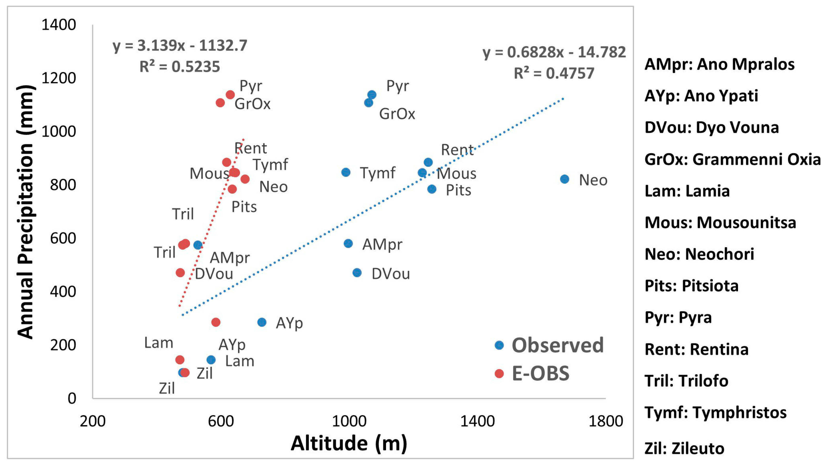
Before the simulations, the reliability of the E-OBS dataset including precipitation and daily temperature (average, minimum and maximum) was evaluated by comparing against time-series of in-situ observations from meteorological stations at the basin. Based on the results, E-OBS dataset systematically underestimated precipitation in Spercheios river basin for the entire period of evaluation. This may be attributed to issues arising in the comparison of in-situ measurements with area-averaged estimates [68], such as the identification of the most representative grid-point for each meteorological station, the insufficient density of the weather stations network in Spercheios river basin or possible uncertainties concerning the accuracy of observational measurements [69]. Moreover, the coarse horizontal resolution of E-OBS prevented to accurately describe the influence of topography on precipitation and to adequately resolve the atmospheric mesoscale processes; 10–15 km grid spacing of meteorological variables generally improves the realism of the results but does not necessarily significantly improve the objectively scored accuracy of the forecasts [70]. Additionally, the coarse network of Greek meteorological stations used in the E-OBS development that are not evenly distributed and do not cover higher altitude sufficiently, eventually does not allow the accurate representation of area-averaged estimates. More specifically, the spatially-averaged annual precipitation calculated at the present study for the period 1960/61–2004/05 was 542.5 mm, which is close to the mean annual precipitation of Lamia meteorological station (585.5 mm for the period 1970–2000 [71]). In other studies, the spatially-averaged annual precipitation of Spercheios river basin was estimated to be 836 mm for the period 2008/09–2010/11 (precipitation estimated based on Thiessen polygons method [72]) and 1,077 mm for the wet hydrological years 2013/14–2014/15 [73] (simulated precipitation provided by Poseidon Monitoring, Forecasting and Information System [74]) [75], while for the period 1949/50–1989/90, the spatially-averaged annual precipitation for Spercheios river basin was estimated to be 904.6 mm [76]. Nevertheless, the main scope of the present study was the trend analysis of the time-series of the main hydrometeorological factors and, therefore, these discrepancies were considered to be acceptable, since no other meteorological data except from the low-altitude Lamia meteorological station (Hellenic National Meteorological Service, WMO 16675) were available for the entire simulation period (1960/61–2004/05).

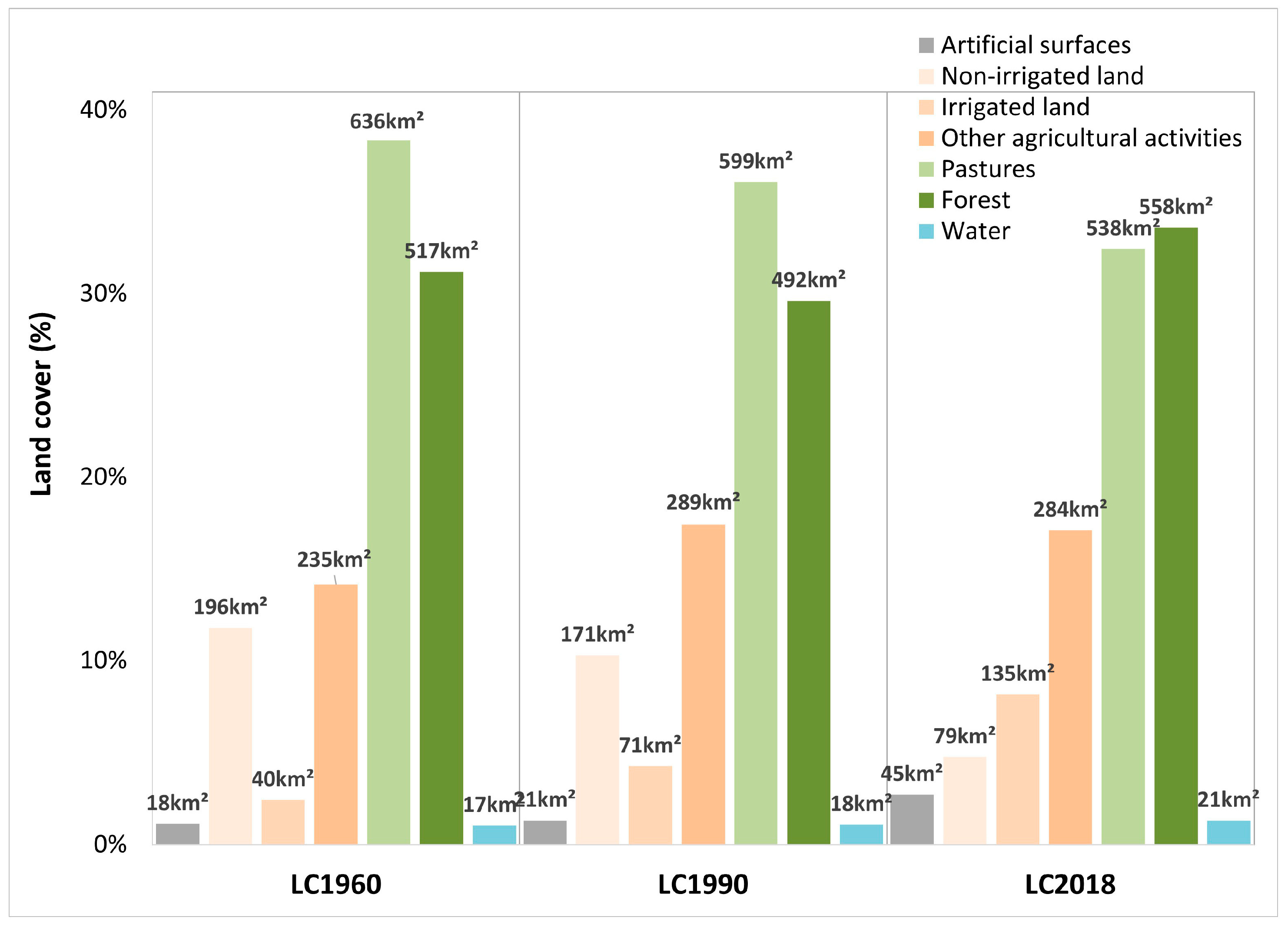
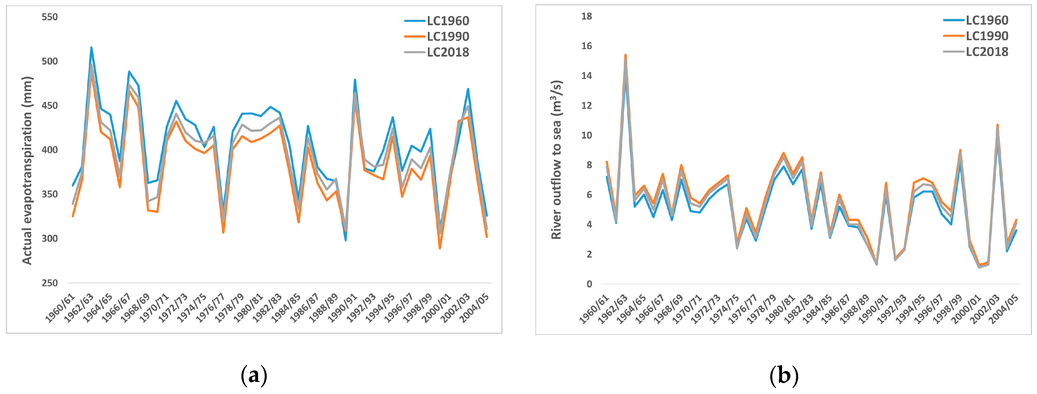
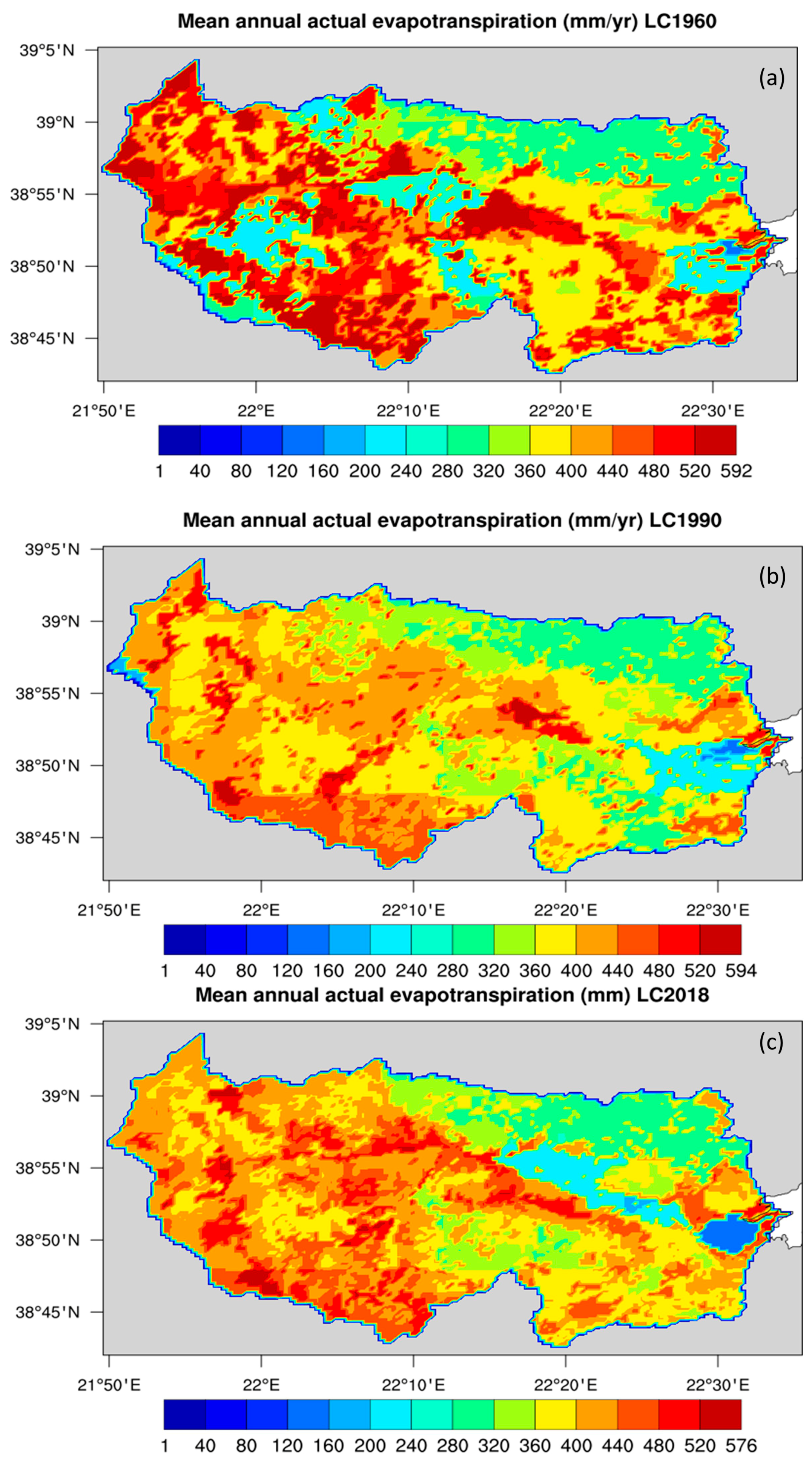
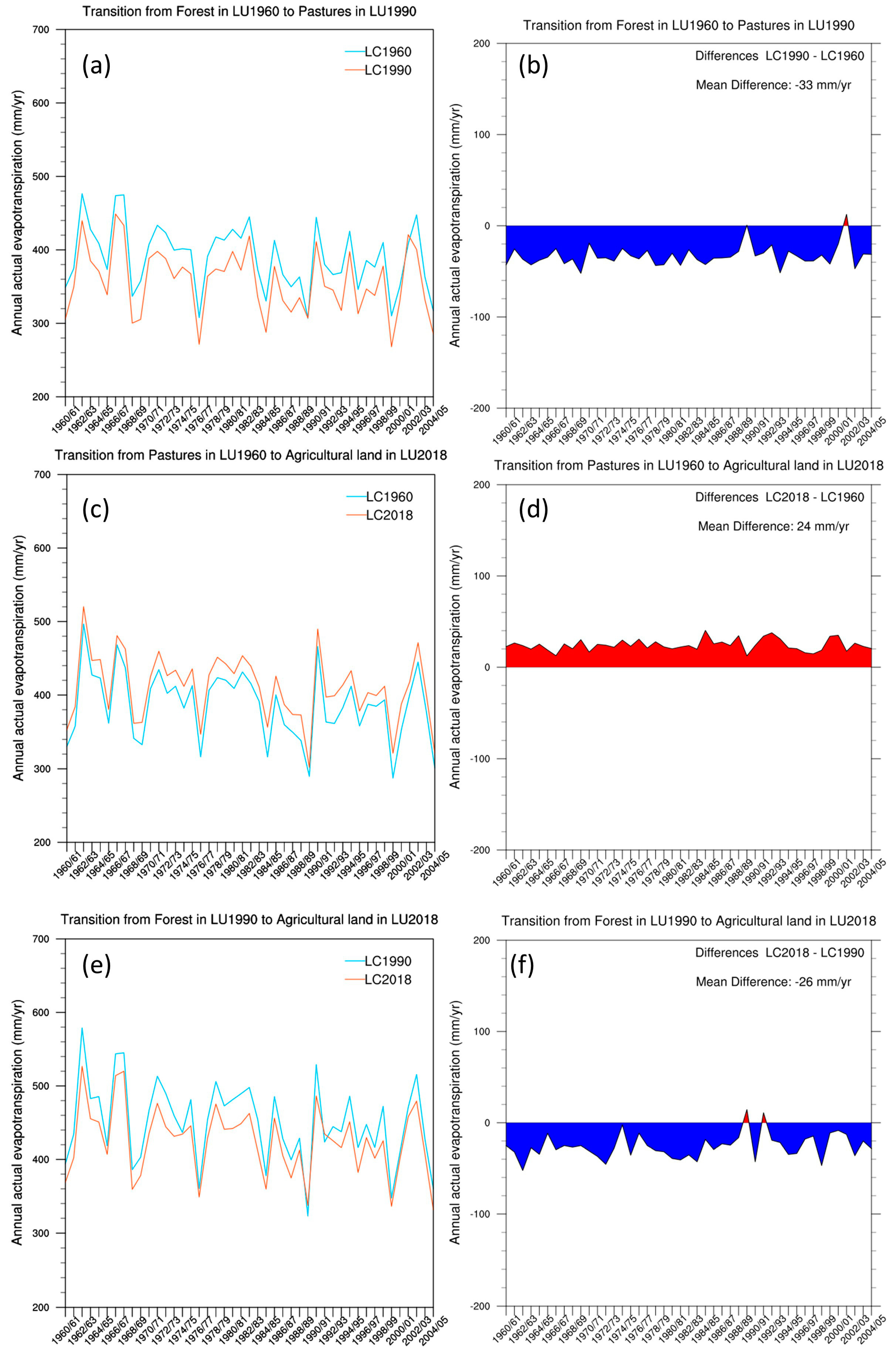
As far as the results of hydrological simulations are concerned, average annual actual evapotranspiration and river discharge were the main parameters of the hydrological cycle which were analyzed in this study. First, the average annual actual evapotranspiration at Spercheios river basin was −5.3% and −2.5% decrease in LC1990 and LC2018 respectively, in comparison to LC1960. These variations can be attributed to the presence of the larger areas covered by vegetation (forest and pastures) in LC1960 (70% in comparison to 66% in LC1990 and LC2018), and especially to the larger extent of areas classified as pastures that also include shrubs, transitional woodland—shrub areas or areas with dense vegetation (38% in LC1960), that led to increased actual evapotranspiration. The higher value of actual evapotranspiration in LC2018 in comparison to LC1990 can be attributed to the increased forested land (34% in LC2018 in comparison to 30% in LC1990). The simulations also presented high spatial differences in average annual actual evapotranspiration. Land cover in 1960 was characterized by a more inhomogeneous pattern than in 1990 and in 2018 due to the increased distribution patterns of areas covered by forests, agricultural land and pastures in 1960 which have different effects on evaporation and transpiration. Moreover, mean annual actual evapotranspiration was almost the same at areas covered by artificial surfaces over time, for example Lamia city, but presents variations where land cover changed. The transition from pastures to agricultural land or forest increased evapotranspiration, while the inverse transition had the opposite effects for the entire simulation period which means that land cover effects can locally outflank the impact of climatic variability.

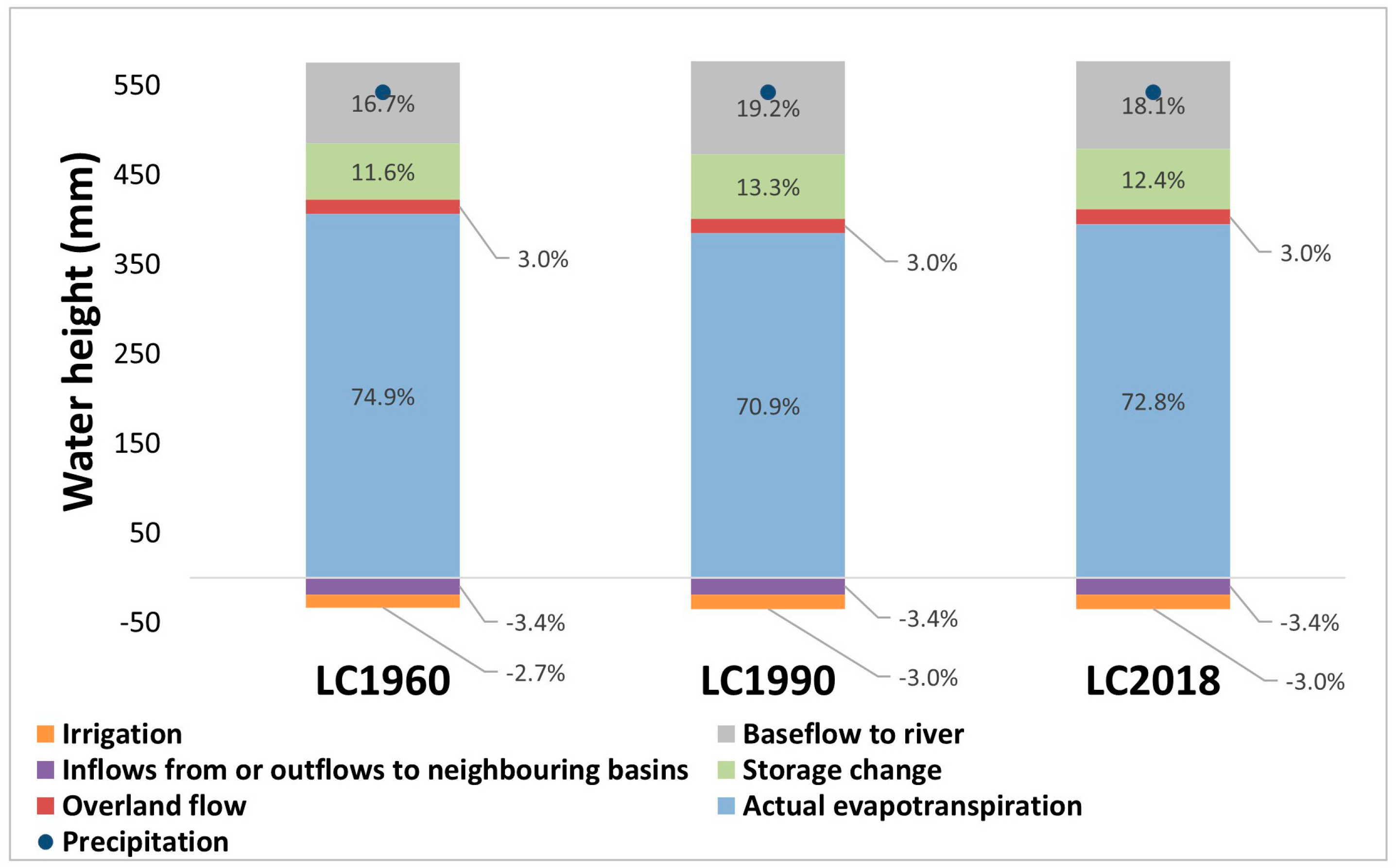
Second, average annual river discharge to Maliakos Gulf was +11.8% and +5.9% increased in LC1990 and LC2018 respectively, in comparison to LC1960. This can partially be attributed to the contribution of the baseflow to river, that ranged from 16.7% in LC1960, through 19.2% in LC1990, to 18.1% in LC2018, following the same pattern. Additionally, the high forested land covering the area of Spercheios river watershed in the case of LC1960 (31%) combined with the lowest irrigation demands during the same period and led to the smallest river discharge. Although in 1990 the forested land slightly decreased (30%), the irrigation demand was almost double, leading to higher exploitation of underground waters, offering residual water in the rivers’ flow and leading eventually to the highest river discharge. Finally, the increase of forested areas in 2018 (34%) and the additional high irrigation demand in 2018 led to the small decrease of river discharge.

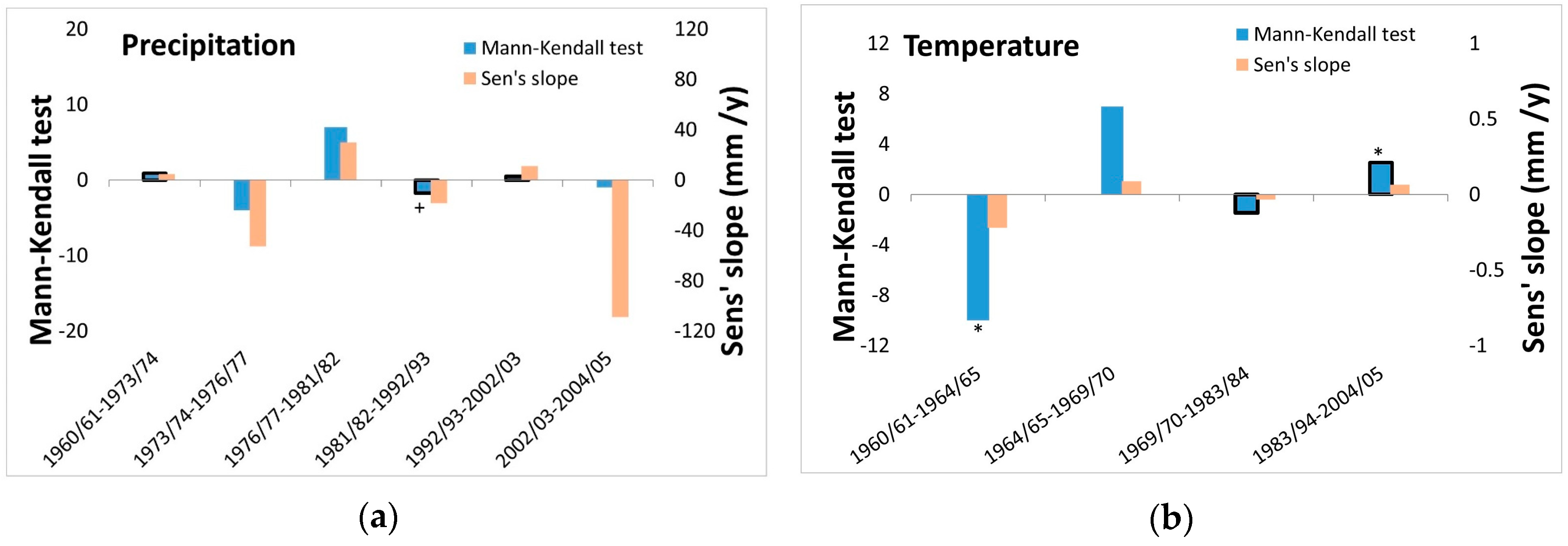
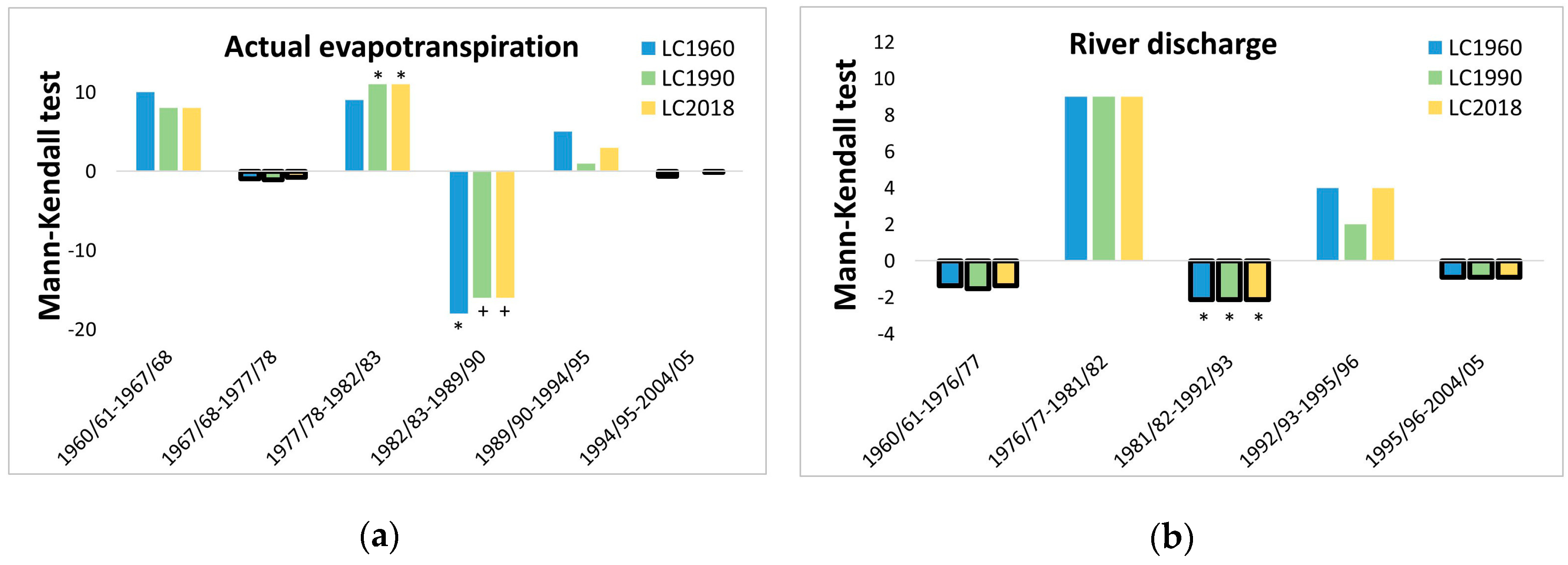
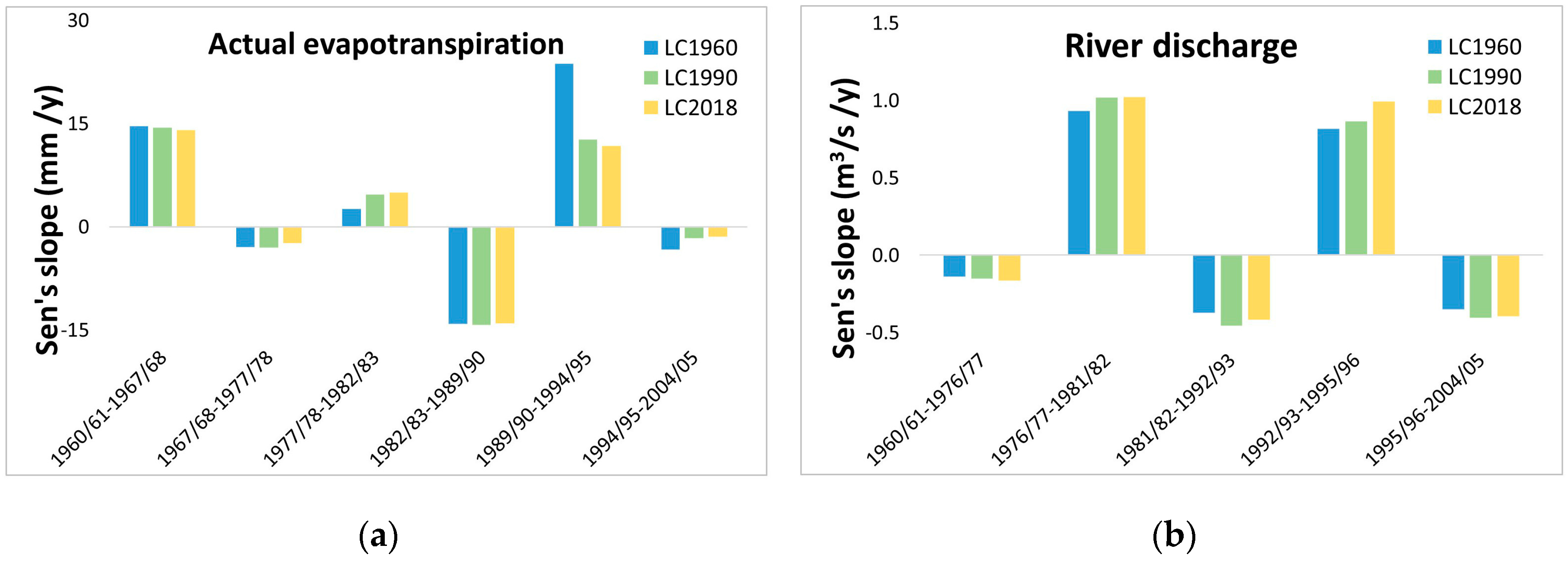
Regarding trend analysis, the effect of land cover change on the trend magnitude was evident. Concerning precipitation and river discharge, the trend change points identified were almost identical. Additionally, the trend change points of actual evapotranspiration identified coincide with those of precipitation, verifying the fact that precipitation is a major factor affecting actual evapotranspiration in dry areas, in contrast to wet areas that evapotranspiration is energy-limited (radiation and air temperature) (for example [77,78,79]). On the contrary, the trend change points of actual evapotranspiration and air temperature were not the same, indicating that actual evapotranspiration is affected in a more complicated way and also by other factors except air temperature as expected, such as land cover and water availability. This was also evident during the trend magnitude analysis of each trend period, where the effect of land cover was noticeable. More specifically, in the case of LC1960, where mean annual actual evapotranspiration was the highest in comparison to the other land cover cases examined, and forested land and pastures (that also include natural grasslands, sclerophyllous vegetation, transitional woodland-shrub, moors and heathland and sparsely vegetated areas) consisted of 70% of the total watershed area, the trend magnitude of each trend period examined was higher. Additionally, highly vegetated watersheds showed smaller tolerance to changes of hydrometeorological factors regarding actual evapotranspiration. On the contrary, the small trend magnitude of river discharge in LC1960 in comparison to LC1990 and LC2018 indicated that in the case of a highly vegetated river basin, the response of the system to changes of hydrometeorological factors regarding river discharge was milder. It is an important finding because land cover of LC1960 could play a relaxing role on the consequences of extreme weather phenomena, either droughts or floods, which will possibly increase in the future.

It should be noted that some uncertainties arise due to the fact that during the present study precipitation and air temperature were considered to be unaffected by land coverage. This is a weakness of the present methodological approach since the current version of the hydrological model MIKE SHE does not provide the option of a two-way dynamically coupled atmospheric-hydrological modeling. The use of an uncoupled system can lead to overprediction of the change in evapotranspiration caused by land cover use changes in comparison to the use of a coupled model results [80].

5. Conclusions

In this study, the physically-based hydrological model MIKE SHE and Copernicus Climate Change Service E-OBS gridded meteorological dataset were used to analyze the effects of anthropogenic land cover changes to the hydrological cycle components of the regional watershed of Spercheios river in central Greece. Three case studies based on the land cover of the years 1960, 1990, and 2018 were investigated.

The analysis of simulation results showed that phenomena like deforestation reduced mean annual actual evapotranspiration while increasing mean annual river discharge. The increase of irrigated agricultural land and irrigation demand also increased discharge as revealed by the results of the case study based on the latest land cover of 2018. Even though irrigation often reduces overland water resources, the exploitation of underground waters can increase river discharge.

Moreover, the climatic variabilities primarily in precipitation and secondarily in temperature influenced annual actual evapotranspiration and annual river discharge. Nevertheless, the response of various watershed areas on land cover changes was shown to be more significant, hiding the effects of climatic variabilities. Land cover changed among the case studies, and thus, locally exceeded the impact of climatic variabilities as indicated by the reduced interannual variabilities of differences in annual actual evapotranspiration. The inhomogeneity of land cover as well as the reduction of vegetated areas were highlighted as the main reasons for this effect.

Remarkably, an in-depth trend analysis unveiled the effect of land cover on increasing the vulnerability on extreme climatic variabilities causing intense hydrometeorological events, either droughts or floods. This means that the resilience of the watershed to extreme weather and climatic phenomena was higher in cases of increased vegetated area, since the response of river discharge in changes of hydrometeorological factors and precipitation was milder in cases of land cover dominated by forested land. This finding highlights the fact that the natural systems under stress mainly due to land cover changes and anthropogenic interventions are likely to have more rapid and acute reactions to climatic variabilities.

Understating the complex interactions among multiple stressors—land degradation and hydrometeorological hazards—can contribute to the development and implementation of successful Integrated Water Resources Management plans. Given the high level of uncertainty of climate change projections and related impacts on water resources, the effects of climatic variabilities on freshwater resources cannot be quantified in a deterministic way; decision-making should be rather based on possible future freshwater hazards and risks. Under this scope, the quantitative assessment of land cover effects presented in this study can be a basis for adaptation and mitigation to climate change and human interventions.

References

1. Kundzewicz, Z.; Krysanova, V.; Benestad, R.; Hov, Ø.; Piniewski, M.; Otto, I. Uncertainty in climate change impacts on water resources. Environ. Sci. Policy 2018, 79, 1–8. [Google Scholar] [CrossRef]
2. Dingman, S.L. Physical Hydrology, 3rd ed.; Waveland Press, Inc.: Long Grove, IL, USA, 2015; Volume 2. [Google Scholar]
3. Zeiringer, B.; Seliger, C.; Greimel, F.; Schmutz, S. River hydrology, flow alteration, and environmental flow. In Riverine Ecosystem Management; Schmutz, S., Sendzimir, J., Eds.; Aquatic Ecology Series 8; Springer: Cham, Switzerland, 2018; pp. 67–89. [Google Scholar]
4. Collier, C.G. Hydrometeorology; John Wiley & Sons, Ltd.: Chichester, UK, 2016. [Google Scholar]
5. Narasimhan, T.N. Hydrological Cycle and Water Budgets. Encycl. Inland Waters 2009, 714–720. [Google Scholar] [CrossRef]
6. Tegen, I.; Fung, I. Contribution to the Atmospheric Mineral Aerosol Load from Land-Surface Modification. J. Geophys. Res. Atmos. 1995, 100, 18707–18726. [Google Scholar] [CrossRef]
7. Cisneros, J.B.E.; Oki, T.; Arnell, N.W.; Benito, G.; Cogley, J.G.; Döll, P.; Jiang, T.; Mwakalila, S. Freshwater resources. In Climate Change 2014: Impacts, Adaptation, and Vulnerability. Part A: Global and Sectoral Aspects. Contribution of Working Group II to the Fifth Assessment Report of the Intergovernmental Panel on Climate Change; Field, C.B., Barros, V.R., Dokken, D.J., Mach, K.J., Mastrandrea, M.D., Bilir, T.E., Chatterjee, M., Ebi, K.L., Estrada, Y.O., Genova, R.C., et al., Eds.; Cambridge University Press: Cambridge, UK; New York, NY, USA, 2014; pp. 229–269. [Google Scholar]
8. Döll, P.; Jiménez-Cisneros, B.; Oki, T.; Arnell, N.W.; Benito, G.; Cogley, J.G.; Jiang, T.; Kundzewicz, Z.W.; Mwakalila, S.; Nishijima, A. Integrating risks of climate change into water management. Hydrol. Sci. J. 2015, 60, 4–13. [Google Scholar] [CrossRef]
9. Brovkin, V.; Boysen, L.; Arora, V.K.; Boisier, J.P.; Cadule, P.; Chini, L.; Claussen, M.; Friedlingstein, P.; Gayler, V.; Van den hurk, B.J.J.M.; et al. Effect of anthropogenic land-use and land-cover changes on climate and land carbon storage in CMIP5 projections for the twenty-first century. J. Clim. 2013, 26, 6859–6881. [Google Scholar] [CrossRef]
10. Poff, N.L.; Allan, J.D.; Bain, M.B.; Karr, J.R.; Prestegaard, K.L.; Richter, B.D.; Sparks, R.E.; Stromberg, J.C. The Natural Flow Regime. Bioscience 1997, 47, 769–784. [Google Scholar] [CrossRef]
11. Haddeland, I.; Heinke, J.; Biemans, H.; Eisner, S.; Flörke, M.; Hanasaki, N.; Konzmann, M.; Ludwig, F.; Masaki, Y.; Schewe, J.; et al. Global water resources affected by human interventions and climate change. Proc. Natl. Acad. Sci. USA 2014, 111, 3251–3256. [Google Scholar] [CrossRef]
12. Wada, Y.; Van Beek, L.P.H.; Bierkens, M.F.P. Modelling global water stress of the recent past: On the relative importance of trends in water demand and climate variability. Hydrol. Earth Syst. Sci. 2011, 15, 3785–3808. [Google Scholar] [CrossRef]
13. Sterling, S.M.; Ducharne, A.; Polcher, J. The impact of global land-cover change on the terrestrial water cycle. Nat. Clim. Chang. 2013, 3, 385–390. [Google Scholar] [CrossRef]
14. Piao, S.; Friedlingstein, P.; Ciais, P.; de Noblet-Ducoudre, N.; Labat, D.; Zaehle, S. Changes in climate and land use have a larger direct impact than rising CO2 on global river runoff trends. Proc. Natl. Acad. Sci. USA 2007, 104, 15242–15247. [Google Scholar] [CrossRef]
15. Blöschl, G.; Ardoin-Bardin, S.; Bonell, M.; Dorninger, M.; Goodrich, D.; Gutknecht, D.; Matamoros, D.; Merz, B.; Shand, P.; Szolgay, J. At what scales do climate variability and land cover change impact on flooding and low flows? Hydrol. Proceses 2007, 21, 1241–1247. [Google Scholar] [CrossRef]
16. Bosmans, J.H.C.; Van Beek, L.P.H.; Sutanudjaja, E.H.; Bierkens, M.F.P. Hydrological impacts of global land cover change and human water use. Hydrol. Earth Syst. Sci. 2017, 21, 5603–5626. [Google Scholar] [CrossRef] [Green Version]
17. Guzha, A.C.; Rufino, M.C.; Okoth, S.; Jacobs, S.; Nóbrega, R.L.B. Impacts of land use and land cover change on surface runoff, discharge and low flows: Evidence from East Africa. J. Hydrol. Reg. Stud. 2018, 15, 49–67. [Google Scholar] [CrossRef]
18. Benjamin, K. Land Use Impacts on Water Resources: A Literature Review; Food and Agriculture Organization of the United Nations-FAO: Rome, Italy, 2000. [Google Scholar]
19. Peel, M.C. Hydrology: Catchment vegetation and runoff. Prog. Phys. Geogr. 2009, 33, 837–844. [Google Scholar] [CrossRef]
20. Dias, L.C.P.; Macedo, M.N.; Costa, M.H.; Coe, M.T.; Neill, C. Effects of land cover change on evapotranspiration and streamflow of small catchments in the Upper Xingu River Basin, Central Brazil. J. Hydrol. Reg. Stud. 2015, 4, 108–122. [Google Scholar] [CrossRef] [Green Version]
21. Arancibia, J.L.P. Impacts of Land Use Change on Dry Season Flows Across the Tropics; King’s College London: London, UK, 2013. [Google Scholar]
22. Chotpantarat, S.; Boonkaewwan, S. Impacts of land-use changes on watershed discharge and water quality in a large intensive agricultural area in Thailand. Hydrol. Sci. J. 2018, 63, 1386–1407. [Google Scholar] [CrossRef]
23. Zhu, C.; Li, Y. Long-Term Hydrological Impacts of Land Use/Land Cover Change From 1984 to 2010 in the Little River Watershed, Tennessee. Int. Soil Water Conserv. Res. 2014, 2, 11–21. [Google Scholar] [CrossRef] [Green Version]
24. Liou, Y.A.; Nguyen, A.K.; Li, M.H. Assessing spatiotemporal eco-environmental vulnerability by Landsat data. Ecol. Indic. 2017, 80, 52–65. [Google Scholar] [CrossRef] [Green Version]
25. Nguyen, A.K.; Liou, Y.A.; Li, M.H.; Tran, T.A. Zoning eco-environmental vulnerability for environmental management and protection. Ecol. Indic. 2016, 69, 100–117. [Google Scholar] [CrossRef]
26. Pikounis, M.; Varanou, E.; Baltas, E.; Dassaklis, A.; Mimikou, M. Application of the SWAT model in the Pinios river basin under different land-use scenarios. Glob. Int. J. 2003, 5, 71–79. [Google Scholar]
27. Varlas, G.; Anagnostou, M.N.; Spyrou, C.; Papadopoulos, A.; Kalogiros, J.; Mentzafou, A.; Michaelides, S.; Baltas, E.; Karymbalis, E.; Katsafados, P. A Multi-Platform Hydrometeorological Analysis of the Flash Flood Event of 15 November 2017 in Attica, Greece. Remote Sens. 2019, 11, 45. [Google Scholar] [CrossRef]
28. Li, G.; Zhang, F.; Jing, Y.; Liu, Y.; Sun, G. Response of evapotranspiration to changes in land use and land cover and climate in China during 2001–2013. Sci. Total Environ. 2017, 596–597, 256–265. [Google Scholar] [CrossRef] [PubMed]
29. Zacharias, I.; Dimitriou, E.; Koussouris, T. Quantifying land-use alterations and associated hydrologic impacts at a wetland area by using remote sensing and modeling techniques. Environ. Model. Assess. 2004, 9, 23–32. [Google Scholar] [CrossRef]
30. UERRA, Uncertainties in Ensembles of Regional ReAnalysis. Available online: http://www.uerra.eu (accessed on 1 June 2019).
31. Copernicus Climate Change Service. Available online: https://climate.copernicus.eu/ (accessed on 1 June 2019).
32. HCMR. Development of an Integrated Management System for Basin, Coastal and Marine Zones. Results of the Annual Evaluation of Ecological Quality of Each Water Body; Hellenic Centre for Marine Research: Anavyssos, Greece, 2015. [Google Scholar]
33. Tselika, V. Form and Development of Prehistoric Settlements in Greece: Spatial Planning and Settlement Patterning. Ph.D. Thesis, Aristotle University of Thessaloniki, Thessaloniki, Greece, 2006. [Google Scholar]
34. Skoulikidis, N.T. The environmental state of rivers in the Balkans—A review within the DPSIR framework. Sci. Total Environ. 2009, 407, 2501–2516. [Google Scholar] [CrossRef]
35. Mentzafou, A.; Vamvakaki, C.; Zacharias, I.; Gianni, A.; Dimitriou, E. Climate change impacts on a Mediterranean river and the associated interactions with the adjacent coastal area. Environ. Earth Sci. 2017, 76, 259. [Google Scholar] [CrossRef]
36. DHI. MIKE SHE User Manual; Danish Hydraulic Institute: Copenhagen, Denmark, 2019. [Google Scholar]
37. Juston, J.; Seibert, J.; Johansson, P.-O. Temporal sampling strategies and uncertainty in calibrating a conceptual hydrological model for a small boreal catchment. Hydrol. Process. 2009, 23, 3093–3109. [Google Scholar] [CrossRef]
38. Vrugt, J.A.; Gupta, H.V.; Dekker, S.C.; Sorooshian, S.; Wagener, T.; Bouten, W. Application of stochastic parameter optimization to the Sacramento Soil Moisture Accounting model. J. Hydrol. 2006, 325, 288–307. [Google Scholar] [CrossRef] [Green Version]
39. Hinkle, D.; Wiersma, W.; Jurs, S. Applied Statistics for the Behavioral Sciences, 5th ed.; Houghton Mifflin: Boston, MA, USA, 2003. [Google Scholar]
40. Moriasi, D.N.; Arnold, J.G.; Van Liew, M.W.; Bingner, R.L.; Harmel, R.D.; Veith, T.L. Model evaluation guidelines for systematic quantification of accuracy in watershed simulations. Trans. ASABE 2007, 50, 885–900. [Google Scholar] [CrossRef]
41. Mentzafou, A.; Wagner, S.; Dimitriou, E. Historical trends and the long-term changes of the hydrological cycle components in a Mediterranean river basin. Sci. Total Environ. 2018, 636, 558–568. [Google Scholar] [CrossRef]
42. National Statistical Service of Greece. Distribution of the Country’s Area by Basic Categories of Land Use. Pre-Census Data (Data for Pre-Census Communal Bulletin of Agriculture and Livestock Census of 19 March 1961); National Statistical Service of Greece: Athens, Greece, 1962. [Google Scholar]
43. Bossard, M.; Feranec, J.; Otahel, J. CORINE Land Cover Technical Guide: Addendum 2000. Technical Report No 40; European Environmental Agency: Copenhagen, Denmark, 2000. [Google Scholar]
44. European Environmental Agency CORINE Land Cover CLC1990, CLC2018 v20b2. Available online: http://land.copernicus.eu/ (accessed on 10 June 2019).
45. Cornes, R.C.; van der Schrier, G.; van den Besselaar, E.J.M.; Jones, P.D. An Ensemble Version of the E-OBS Temperature and Precipitation Data Sets. J. Geophys. Res. Atmos. 2018, 123, 9391–9409. [Google Scholar] [CrossRef] [Green Version]
46. Hofstra, N.; Haylock, M.; New, M.; Jones, P.D. Testing E-OBS European high-resolution gridded data set of daily precipitation and surface temperature. J. Geophys. Res. Atmos. 2009, 114. [Google Scholar] [CrossRef]
47. Copernicus Climate Change Service (C3S) Ensembles User Guide. Available online: http://surfobs.climate.copernicus.eu/userguidance/use_ensembles.php (accessed on 1 June 2019).
48. Klok, E.J.; Tank, A.M.G.K. Updated and extended European dataset of daily climate observations. Int. J. Climatol. 2009, 29, 1182–1191. [Google Scholar] [CrossRef]
49. Van Engelen, A.; Klein Tank, A.; van der Schrier, G.; Klok, L. Towards an operational system for assessing observed changes in climate extremes. In European Climate Assessment & Dataset (ECA&D), Report 2008; KNMI: De Bilt, The Netherlands, 2008. [Google Scholar]
50. Hargreaves, G.H.; Samani, Z.A. Reference Crop Evapotranspiration from Temperature. Appl. Eng. Agric. 1985, 1, 96–99. [Google Scholar] [CrossRef]
51. Shuttleworth, W.J. Evaporation. In Handbook of Hydrology; Maidment, D.R., Ed.; McGraw-Hill Book Company: New York, NY, USA, 1993; pp. 4.1–4.53. [Google Scholar]
52. Koutsoyiannis, D.; Xanthopoulos, T. Engineering Hydrology, 3rd ed.; National Technical University of Athens: Athens, Greece, 1999. [Google Scholar]
53. National Statistical Service of Greece. Results of Agriculture and Livestock Census of March 19th 1961. Volume I, Issue 2: Central Greece and Evoia; National Statistical Service of Greece: Athens, Greece, 1965. [Google Scholar]
54. National Statistical Service of Greece. Census of Agricultural and Livestock Holdings 2010; National Statistical Service of Greece: Athens, Greece, 2014. [Google Scholar]
55. Savva, A.P.; Frenken, K. Crop water requirements and irrigation scheduling. In Irrigation Manual Module 4; Water Resources Development and Management Office, FAO Sub- Regional Office for East and Southern Africa: Harare, Zimbabwe, 2002; Volume 4. [Google Scholar]
56. National Statistical Service of Greece. Agricultural Statistics of Greece. Year 1990; National Statistical Service of Greece: Athens, Greece, 1994. [Google Scholar]
57. National Statistical Service of Greece. Annual Agricultural Stiatistical Survey: 2017; National Statistical Service of Greece: Athens, Greece, 2018. [Google Scholar]
58. Sneyers, R. On the Statistical Analysis of Series of Observations. Technical Note no. 143; World Meteorological Organization: Geneva, Switzerland, 1990. [Google Scholar]
59. McGilchrist, C.A.; Woodyer, K.D. Note on a distribution-free CUSUM technique. Technometrics 1975, 17, 321–325. [Google Scholar] [CrossRef]
60. Page, E.S. Continuous Inspection Schemes. Biometrika 1954, 41, 100–115. [Google Scholar] [CrossRef]
61. Montgomery, D.C. Introduction to Statistical Quality Control, 6th ed.; John Wiley & Sons, Inc.: New York, NY, USA, 2009. [Google Scholar]
62. Mann, H.B. Nonparametric tests against trend. Econometrica 1945, 13, 245–259. [Google Scholar] [CrossRef]
63. Kendall, M.G. Rank Correlation Methods; Charles Griffin and Company: London, UK, 1975. [Google Scholar]
64. Gilbert, R.O. Statistical Methods for Environmental Pollution Monitoring; Van Nostrand Reinhold Co.: New York, NY, USA, 1987. [Google Scholar]
65. Sen, P.K. Estimates of the regression coefficient based on Kendall’s Tau. J. Am. Stat. 1968, 63, 1379–1389. [Google Scholar] [CrossRef]
66. Machiwal, D.; Jha, M. Hydrologic Time Series Analysis: Theory and Practice; Springer: Dordrecht, The Netherlands, 2012. [Google Scholar]
67. Brooks, K.N.; Ffolliott, P.F.; Magner, J.A. Hydrology and the Management of Watersheds, 4th ed.; Wiley-Blackwell: Ames, IA, USA, 2012. [Google Scholar]
68. Papadopoulos, A.; Katsafados, P. Verification of operational weather forecasts from the POSEIDON system across the Eastern Mediterranean. Nat. Hazards Earth Syst. Sci. 2009, 9, 1299–1306. [Google Scholar] [CrossRef] [Green Version]
69. Servuk, B. Spatial and temporal inhomogeneity of global precipitation data. In Global Precipitations and Climate Changes. Proceedings of the NATO Advanced Research Workshop on Global Precipitations and Climate Change, La Londe les Maures, France, 27 September–1 October 1993; Desbois, M., Desalmand, F., Eds.; Springer: Berlin/Heidelberg, Germany, 1994; Volume 57, pp. 219–230. [Google Scholar]
70. Mass, C.F.; Ovens, D.; Westrick, K.; Colle, B.A. Does increasing horizontal resolution produce more skillful forecasts? The results of two years of real-time numerical weather prediction over the Pacific Northwest. Bull. Am. Meteorol. Soc. 2002, 83, 407–430. [Google Scholar] [CrossRef]
71. Psomiadis, E. Research of Geomorphological and Environmental Changes in the Sperchios’ River Basin Utilizing New Technologies. Ph.D. Thesis, Agricultural University of Athens, Athens, Greece, 2010. [Google Scholar]
72. Thiessen, A.H. Precipitation averages for large areas. Mon. Weather Rev. 1911, 39, 1082–1084. [Google Scholar] [CrossRef]
73. Tolika, K.; Maheras, P.; Anagnostopoulou, C. The exceptionally wet year of 2014 over Greece: A statistical and synoptical-atmospheric analysis over the region of Thessaloniki. Theor. Appl. Climatol. 2018, 132, 809–821. [Google Scholar] [CrossRef]
74. Papadopoulos, A.; Katsafados, P.; Kallos, G.; Nickovic, S. The weather forecasting system for POSEIDON—An overview. Glob. Atmos. Ocean Syst. 2002, 8, 219–237. [Google Scholar] [CrossRef]
75. HCMR. Development of an Integrated Management System for Basin, Coastal and Marine Zones. Hydrological and Hydrochemical Model of the Study Area; Hellenic Centre for Marine Research-Institute of Marine Biological Resources and Inland Waters: Anavyssos, Greece, 2015. [Google Scholar]
76. Ministry of Develpmenet-NTUA-Institute of Geological and Mining Research-Centre for Research and Planning. Master Plan for Water Resource Management of the Country; Ministry of Develpmenet: Athens, Greece, 2003.
77. Milly, P.C.D.; Dunne, K.A. Trends in evaporation and surface cooling in the Mississippi River basin. Geophys. Res. Lett. 2001, 28, 1219–1222. [Google Scholar] [CrossRef]
78. Gao, G.; Chen, D.; Xu, C.Y.; Simelton, E. Trend of estimated actual evapotranspiration over China during 1960–2002. J. Geophys. Res. Atmos. 2007, 112. [Google Scholar] [CrossRef]
79. Yang, K.; Ye, B.; Zhou, D.; Wu, B.; Foken, T.; Qin, J.; Zhou, Z. Response of hydrological cycle to recent climate changes in the Tibetan Plateau. Clim. Chang. 2011, 109, 517–534. [Google Scholar] [CrossRef]
80. Overgaard, J.; Butts, M.; Rosbjerg, D. Improved scenario prediction by using coupled hydrological and atmospheric models. In Quantification and Reduction of Predictive Uncertainty for Sustainable Water Resources Management: Proceedings of Symposium HS2004 at IUGG 2007, Perugia, July 2007. IAHS Publ. 313; Boegh, E., Kunstmann, H., Wagener, T., Hall, A., Bastidas, L., Franks, S., Gupta, H., Rosbjerg, D., Schaake, J., Eds.; IAHS Press: Wallingford, UK, 2007; pp. 242–248. [Google Scholar]
Figure 1. Study area.
Climate 07 00129 g001
Figure 2. Flowchart of the current methodological approach.
Climate 07 00129 g002
Figure 3. Land cover maps for the year: (a) 1960 produced for the present study, (b) 1990, and (c) 2018 from CORINE Land Cover (CLC).
Climate 07 00129 g003
Figure 4. Distribution of land cover type for the three land cover case studies examined.
Climate 07 00129 g004
Figure 5. Differences in agricultural land (a), pastures (b) and forests (c) for the three land cover case studies examined.
Climate 07 00129 g005
Figure 6. Precipitation lapse rates of Spercheios river basin based on observational meteorological data and E-OBS dataset.
Climate 07 00129 g006
Figure 7. Basin-averaged annual actual evapotranspiration (mm) (a) and river discharge (m3/s) to Maliakos Gulf (b) reconstructions. LC1960, LC1990 and LC2018 are represented by blue, orange and gray lines.
Climate 07 00129 g007
Figure 8. Simulated mean annual actual evapotranspiration (mm/yr) in (a) 1960, (b) 1990 and (c) 2018.
Climate 07 00129 g008
Figure 9. Timeseries, regarding areas characterized by transition from forest in 1960 to pastures in 1990, of (a) annual actual evapotranspiration (mm/yr) simulated by LC1990 (orange line) and LC1960 (blue line) as well as (b) their differences (red for positive and blue for negative). The same for (c,d) as well as (e,f) regarding transition from pastures in 1960 to agricultural land in 2018 and transition from forest in 1990 to agricultural land in 2018, respectively.
Climate 07 00129 g009
Figure 10. SMK and CUSUM tests for (a) precipitation and (b) air temperature.
Climate 07 00129 g010
Figure 11. Results of Mann-Kendall test (No border in columns indicates S test and black border Z test; (*) and (+) symbols indicate if trend is significant at α = 0.05 level and at α = 0.1 level respectively) and Sen’s slope for (a) precipitation and (b) air temperature.
Climate 07 00129 g011
Figure 12. SMK and CUSUM tests for actual evapotranspiration for (a) LC1960, (b) LC1990, and (c) LC2018, and river outflow to Maliakos Gulf for (d) LC1960, (e) LC1990, and (f) LC2018.
Climate 07 00129 g012
Figure 13. Results of Mann-Kendall test for actual evapotranspiration (a) and river discharge (b) for LC1960, LC1990, and LC2018. No border in columns indicates S test and black border Z test. (*) and (+) symbols indicate if the trend is significant at the α = 0.05 level and α = 0.1 level, respectively.
Climate 07 00129 g013
Figure 14. Sen’s slope for actual evapotranspiration (a) and river discharge (b) for LC1960, LC1990, and LC2018.
Climate 07 00129 g014
Figure 15. Water budget of Spercheios river basin for the three land cover case studies examined.
Climate 07 00129 g015