I. Introduction

The power of observing significant snow and ice features with satellites was first demonstrated when television cameras with relatively modest spatial resolution, mounted on the TIROS-2 weather satellite, monitored the breakup in the Gulf of St, Lawrence during Spring 1961. In that case, only one of several advantages of remote sensing from satellites was brought to bear on the problem of monitoring sea ice; namely, the ability to obtain almost instantaneously a synoptic view over large areas. Figure 1 demonstrates this capability showing a mosaic made from the Nimbus 3 image dissector camera system (IDCS) on 15 April 1969. Large areas of north-eastern Canada, Baffin Island, Greenland, and Iceland can be seen quite clearly.

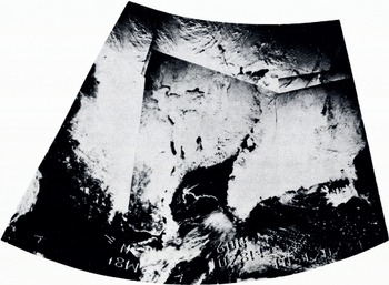
Fig. 1. Satellite photograph of snow and ice conditions in Iceland, Greenland, east Canada, and. New England, is April 1969.

Observations in many other spectral regions have been made since the visible wavelength TIROS-2 observations were made. These observations in other spectral regions have made it possible to monitor repetitively over extensive areas many important properties of snow and ice that are and have been applied in a useful fashion to many practical situations including navigation and water resources monitoring. In 1964, for instance, Nimbus-1 obtained the first images of infrared emission in the 3.8 μm region over Antarctica. Because of the strong contrast in temperature between ice and open water, breaks in the sea ice could be monitored in night-time conditions that occur continuously over polar areas during the winter months.

Observations from the Nimbus-3 high resolution infrared radiometer in the 0,7-1.3 μm spectral region illustrated the utility of these data for delineating regions where active melting was occurring on ice and snow and thus decreasing the reflectance in this spectral region. Figure a taken from Nimbus-3 graphically illustrates this in simultaneous views over the southern Sierra Nevada Mountains region in California.

The long life (1-3 years) of Nimbus and NOAA satellites of the late 1960’s and early 1970’s has permitted reliable, repetitive snow-cover observations of utility for snow-pack monitoring and subsequent run-off prediction. Reference Barnes and BowleyBarnes and Bowley (1968) and Reference McClain and BakerMcClain and Baker (1969) have described techniques for analyzing and presenting snow-cover observations from meteorological satellites. Figure 3 shows repetitive observations taken by the Nimbus 3 and 4 IDCS over the Indus River basin in the Himalayan region of south-west Asia. Salomon-son and MacLeod (1972) (Fig. 4) showed evidence that these observations may have a usable empirical relationship to observed run-off that could be used for seasonal or monthly run-off prediction in areas lacking conventional information. The IDCS has also been used to provide maps of the polar regions on occasions when cloud obscuration was not a problem. An example of such imagery is shown in Figure 5 in which the continent of Antarctica was observed during a series of satellite overpasses on relatively cloud-free days. The outline of the continent is fairly clearly seen. However, the signature of the continent itself is quite uniform except for scattered cloud formations and a few mountain ridges. Unlike the images obtained in snow-covered areas outside the polar regions, there is no bare ground or forestation to provide distinguishable details.

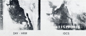
Fig. 2. Simultaneous views of the southern Sierra. Nevada Mountains in California obtained in the visible (LDCS) and near-infrared (HRIR) spectral regions.

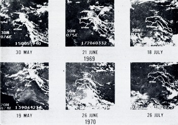
Fig. 3. Nimbus-3 and. Nimbus-4 IDCS observations of snow cover over the Indus River watershed during the major snow-melt period.

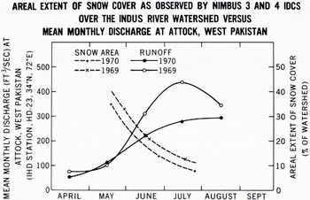
Fig. 4. Aerial extent of snow cover over the Indus River watershed as obtained by the analysis of the images in Figure 3. 500 ft³/s = 14.2m³/s.

In summary, the early meteorological satellites, TIROS, Nimbus, and ITOS or NOAA provide, or have provided, results of interest and utility for monitoring snow and ice features synoptically over large areas in the visible, near infrared (0.7-1.3 μm), and far infrared (3.8 and 10-12 μm) with modest spatial resolution (in general, > 4km). In the last two years, however, at least two significant breakthroughs in global snow and ice monitoring were made. These involve the relatively high resolution (80 m) observations in the visible and near infrared from the Earth Resources Technology Satellite, ERTS-I, and observations in the microwave portion of the electromagnetic spectrum obtained from the Nimbus-5 spacecraft. The following sections describe representative and relevant results from these two spacecraft.

II. ERTS-I Results

ERTS-I was launched on 23 July 1962 into a near polar, sun-synchronous orbit at an altitude near 900 km. The orbital characteristics are nominally such that the multi-spectral scanner subsystem (MSS) on ERTS-I is capable of taking observations of cartographic quality in the 0.5-0.6, 0.6-0.7, 0.7-0.8 and 0.8-1.1 μm spectral regions over any given point on Earth once every 18 d, cloud cover and sunlight permitting. The convergence of the orbits at high latitudes makes it possible to monitor individual ice floes, cracks and leads, polynyas, and icebergs more often than 18 d and in some areas features can be monitored on daily intervals. Results from analysis of ERTS-I data involving snow and ice mapping are provided in Reference FredenFreden and others (1973) and a review is provided by Reference Salomonson and GreavesSalomonson and Greaves (1974).

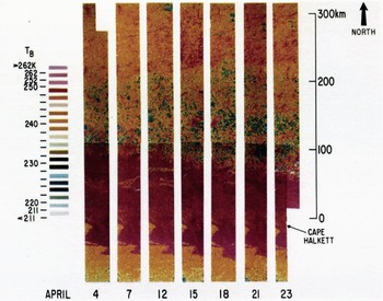
Fig. 7. Time sequence of microwave (λ — 1.55 cm) mosaic maps of sea ice in the southern Beaufort Sea. The maps extend from Cape Halkett on the western side of Harrison Bay north for approximately 350 km

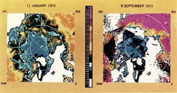
Fig. 9. Seasonal changes in the extent of the Arctic icepack as shown in the ESMR imagery (false color).

Fig. 11. Three sequential ESMR images of the Antarctic showing the rapid development of major polynyas and leads: A. 18 November 1973, B. 27 November 1973, and C. 9 December 1973.

Fig. 12. False-color representations of the passive microwave imagery (1.55 cm) from the sea-ice test areas studied by the U.S team during BESEX. The mosaics were assembled in a computer from the individual data points obtained during the five-track aircraft flight pattern. The regions of elongated color strips represent periods of instrumentation malfunction (Gloersen and others, 1974[b]).

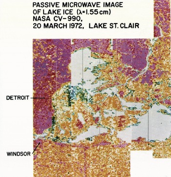
Fig. 13. Passive microwave image (λ = 7.55 cm) of lake ice in Lake St. Clair on So March 1972- The brightness temperature corresponding to the uniform grey tone indicates open water. Where the colors show light and dark blues (cold) the ice is thinner than where the colors indicate red, violet, and orange (warmer).

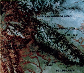
Fig. 6. False-color composite view of Wind River Mountains of Wyoming obtained from the ERTS-I satellite, G Angust 1972. Watershed boundaries are indicated, those in blue < 10 000 ft (3 050 m), those in black > 10 000 ft (3 050 m) mean elevation.

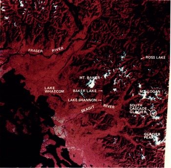
Fig. 8. An ERTS-I 185 km X 185 km image reproduced from observations acquired on 16 September 1973 over Washington State. South Cascade Glacier appears at the lower right.

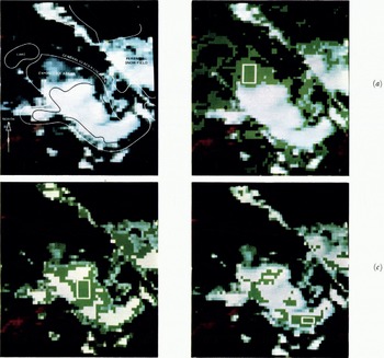
Fig. 9. Expanded views of South Cascade Glacisr· Digital data from the o.5-0.6 μm 0.6-0.7 μm, and 0.8-1. l μm imagery was displayed on a television screen and photographed and parallelepiped classifications performed.

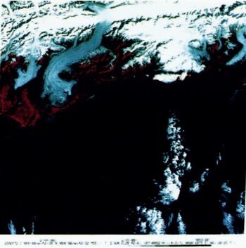
Fig. 10. Three ERTS-I 185 km X 185 km images over the Bering Glacier in south-central Alaska.

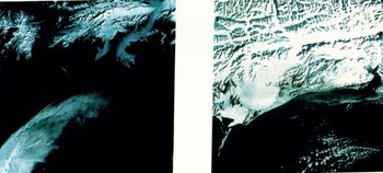
Fig. 11. Two views of the Bering Glacier showing a partially classified scene (left) and the selected areas used to classiff more completely the same scene (right) (ERTS-I 22 September 1973).

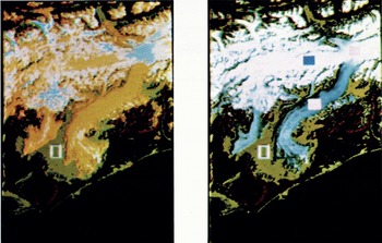
Fig. 13. Image of the Ross Ice Shelf region in Antarctica obtained from the ERTS-I satellite.

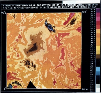
Fig. 14. Image of Antarctica obtained from the Nimbus-5 THIR on 11 January 1973.

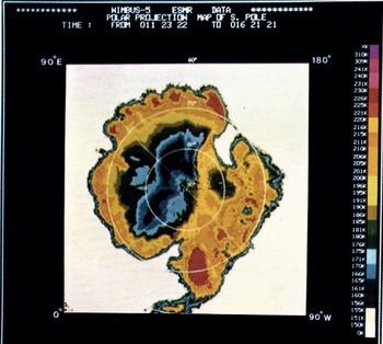
Fig. 15. Imaige of Antarctica obtained from the. Nimbus-5 ESMR averaged over five, days starting on 11 January 1973.

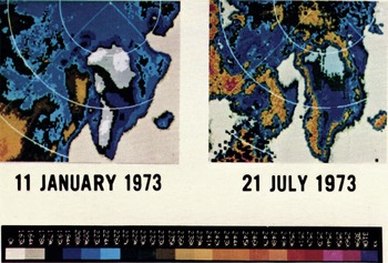
Fig. 19. The image of Greenland obtained from 1.55 cm microwave data for the summer and winter seasons (11-16 January 1973 and 21 July 1973)·

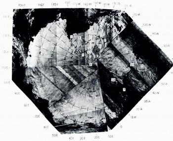
Fig. 5. Nimbus-4. IDCS observation of Antarctica. Marked stations and camps are as follows: 1: McMurdo (U.S.A.) and Scott Base (New Zealand),2: "Byrd" (U.S.A.). 3: South Pole (U.S.A.). 4: "Hallett" (U.S.A.). 5: "Brockton". (U.S.A.). 6: "Vostok" (U.S.S.R.). 7: Halley Bay (U.K.). 8: "Siple" (U.S.A.). 9: "McGregor" (U.S.A.). 10; "Lassiter" (U.S.A.). 11: "Amundsen" (U.S.A.). 12: "Shackleton" (U.K.). 13: Dronning Maud (Norway).

In terms of snow-pack monitoring, activities at Goddard Space Flight Center have centered on the use of ERTS-I data in the Wind River Mountains of Wyoming. The principal objective has been to see if snow-cover area observations may be useful in empirical fashion to better characterize and perhaps predict run-off from watersheds in these mountains. Figure 6 (pl. IV) shows how the Wind River Mountain area appears from ERTS-I. Watershed boundaries for seven watersheds in which snow-mapping from ERTS has been accomplished are delineated on this figure. Three of the watersheds have mean elevations above 3 km and four of the watersheds have mean elevations below 3 km.

During the 1973 snow-melt season several cloud-free views of the watersheds mentioned above were obtained. The percentage of each basin covered by snow was plotted versus time along with the variation in the 18 d mean flow per unit area for each of these watersheds. In order to see if it is possible to demonstrate that major physiographic differences affect the character of snow-cover depletion curves, the results for the three high watersheds and the four low watersheds were compiled and average results obtained. The normalizing factors used in comparing the results consisted in using specific run-off (per unit area) rather than the total volume of run-off. The results of this procedure are shown in Figure 7. The principal point to be made concerning this figure is that the general character of the specific run-off and snow-cover variation between high and low watersheds (mean elevation >3 km and <3 km respectively) can be seen to be distinctly different. The specific run-off from the lower watersheds has a smaller peak flow that occurs earlier in time. These characteristics are consistent with the snow-cover depletion curve which shows the snow cover disappearing more rapidly with time due to smaller snow depths and the higher temperatures at the lower altitudes. Of course, several years of data are necessary in order to establish rigorously the utility of this kind of approach for a given watershed. Along these lines, analyses of the 1974 ERTS-I snow-cover observation are continuing.

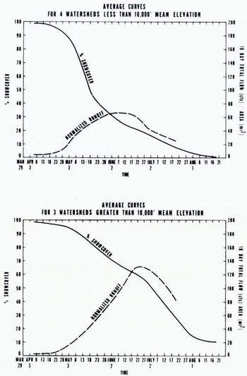
Fig. 7. Average. snow-caver depletion and run-off for the Wind River Mountain watersheds during 1973 as obtained by analyzing ERTS images such as those shown in Figure 6. 200 ft³/s mi² =.1. 09 m³/s km².

The ERTS-I data have been found to be particularly exciting for the monitoring and study of glaciers and their attendant surface features. The character of medial and terminal moraines, the extent of snow cover, debris, and other features can be observed repeatedly and related to the mass balance of the glacier and its movement. Of particular interest has been the use of these observations to locate or monitor surging glaciers. The Yentna Glacier near Mt McKinley, Alaska, and the Tweedsmuir Glacier in British Columbia, Canada, are among those glaciers of this type whose recent surges have been monitored from ERTS-I.

Not a great deal of analysis has been accomplished and reported in the recent literature in which ERTS-I digital data and objective feature classification have been employed in glaciological studies. The utilization of digital data commonly allows one to extract more detail and analytical numerical information than one can obtain simply from photographic enlargement and processing. To illustrate these points, ERTS scenes taken over the Bering Glacier (lat. 60° N., long. 144° W.) in south-central Alaska and the South Cascade Glacier (lat. 48° 30’ N., long. 121° W.) in Washington state were examined using ERTS digital data stored on computer compatible tapes. Figure 8 (pl. VI) shows the entire 185 km X 185 km color composite image taken over Washington State on 16 September 1973. The location of the South Cascade Glacier is outlined by a small circle covering an area that is approximately 6.5 km in diameter.

Figure 9 (pl. V) shows this same area expanded many times so that more detail can be seen than is discernible on the previous figure. Sketch lines have been superimposed to show the areal extent of major features in this expanded view of the glacier. Portions a, b, and c of Figure 9 show what portions of the glacier appear to have the same multispectral character as each of the small areas enclosed in the white rectangles. By this, we mean that the digital reflectance values obtained for the 0.5-0.6, 0.6- 0.7, and 0.8-1.1 μm band MSS observations agree within a pre-specified tolerance. In Figure 9a, b, and c, all areas that appeared the same as the selected areas are displayed as a green color. Using such data-processing equipmentFootnote ^* one can select a known area and in a few seconds classify the remainder of the scene to see how many other areas are similar in a multi-spectral sense. Also, one can measure areas or obtain other statistical information that may be appropriate. As another example, Figure 10 (pl. V-VI) shows three 185 km X 185 km color composite views of the Bering Glacier reflecting seasonal and annual changes. Figure 11 (pl. VI) shows a partially classified September 1972 scene depicting selected areas in various colored squares and a more completely classified scene employing each of the selected samples. The classifications represent the more debris-laden, exposed ice portions of the glacier (area marked by white, open square), the cleaner, less debris-covered, exposed ice portions of the glacier (white solid square) and the snow-covered regions of the snow fields feeding the glacier (blue, solid square). These classifications or variations thereof can be accomplished in only a few minutes and quantitative supporting data provided shortly thereafter such as the number of data elements, or the area comprising each classification.

III. Nimbus-5 Results

Nimbus-5 was launched on 11 December 1972 into a near polar sun-synchronous circular orbit at an altitude of about 1 too km. In addition to the infrared and microwave atmospheric sounders on board, the spacecraft contains three imaging devices in the infrared and microwave regions. The highest spatial resolution is achieved by the surface composition mapping radiometer (SCMR) which has three spectral intervals from 8.3-9.3 μm, 10.2-11.2 μm and 0.8-1.1 μm. The instantaneous field of view of this instrument is 0.6 mrad providing a nadir ground resolution cell size of about 660 m. An example of the imaging quality available from this device is shown in Figure 12 which depicts the Ross Ice Shelf in Antarctica. The structural detail shown in this image is excellent, but the technique suffers for significant fractions of the observing time from obscuration by cloud cover. Features evident in this figure include open water in the Ross Sea, bare terrain in the McMurdo area, and scattered clouds. As in the IDCS image (Fig. 5), the structural details on the continental ice sheet are lacking. Increasing the spatial resolution apparently does not help in bringing out the details in the ice sheet as is shown from the ERTS image of the McMurdo area in the Ross Sea (Fig. 13, pl. VII). While the open water, bare terrain, and bare glaciers are clearly depicted, it is evident that as the higher elevations are reached the details become less and less pronounced.

The temperature-humidity infrared radiometer (THIR) is a two-channel scanning radiometer with considerably lower spatial resolution. One channel ranges from 6-5-7 μm with a 21 mrad field of view, and the other from 10.5-12.5 μm with a 7 mrad field of view. The latter channel is used for observing the surface in the absence of clouds. THIR provides valuable information on surface temperature when atmospheric conditions permit. In Figure 14 (pl. VII), there is shown a polar stereographic projection of THIR data from the 10.5-12.5μm channel of the South Polar region. In this image, the continent of Antarctica was largely cloud-free except in the region of the Ross Ice Shelf where a cloud system intruded over the continent from the South Pacific Ocean. Generally speaking, however, the edge of the floating ice pack is obscured by persistent cloud cover in this image. Also, the continental outline is not clearly depicted.

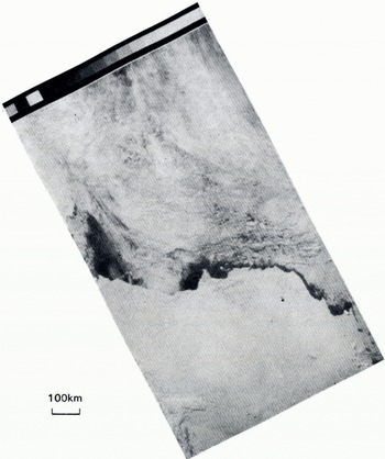
Fig. 12. Image of a portion of the Ross he Shelf region in Antarctica obtained from the Nimbus-5 SCMR. Ross Island is near the center of the left-hand edge of the image. The other extremity of the ice, shelf edge is about ⅜ of the image width from the left-hand edge.

The electronically scanned microwave radiometer (ESMR) on board the Nimbus 5 provides daily coverage over both the polar regions. The ESMR receives radiation emanating from the Earth at a wavelength of 1.55 cm. In this wavelength region and over the temperatures encountered, the Rayleigh-Jeans approximation to the radiation law applies. That is, the radiative power received is proportional to the first power of the brightness temperature of the radiator which, in turn, is a product of the physical temperature of the radiator and its emissivity. Thus the images produced by the ESMR contain information both on the temperature variation over the surface of the Earth and the variation of the emissivity for different Earth surfaces. Radiation received at 1.55 cm originates both from the atmosphere of the Earth and its surface. In particular, the atmospheric contributions come both from water vapor (the wing of the 22.2 GHz water-vapor line) and from liquid water in clouds. Only under conditions of extensive heavy rainfall does the entire contribution come from the atmosphere. The applications of the ESMR imagery in terms of meteorological phenomena over the oceans have been described by Reference Wilheit, Wilheit, Theon, Shenk and AllisonWilheit and others (1973). The atmospheric contribution is the greatest in the tropical regions. In the Arctic and Antarctic, the liquid water and water-vapor contributions become negligible so that the surface can be observed all the time.

The utility of the ESMR in observing sea ice and continental sheet ice has been described previously (Gloersen and others, 1973[a], [b]; Reference Campbell, Campbell, Gloersen, Nordberg, Wilheit and BockCampbell and others, 1974). Dr Campbell will discuss in some detail in another paper at this symposium (Reference Campbell, Campbell, Weeks, Ramseier and GloersenCampbell and others, 1975) the sea-ice data obtained in the Arctic and Antarctic regions from the ESMR. For the purposes of illustrating the utility of this technique. Figure 15 (pl. VIII) shows an image of the South Polar region for the same date on which the THIR image was shown in Figure 14. The sea ice surrounding Antarctica appears to have the characteristics of first-year ice, that is, ice with salinity content of 1‰ or more in the freeboard portion of the ice. The emissivity of such ice is 0.95 or greater at a wavelength of 1.55 cm based on aircraft measurements in the Arctic area (Gloersen and others, I973[a], 1974). The fact that this signature is present in the Weddell Sea is surprising inasmuch as the ice pack in this region persists from one year to the next, according to the ESMR data acquired since November 1972 and the observations of workers in the field (private communication from W. F. Weeks).

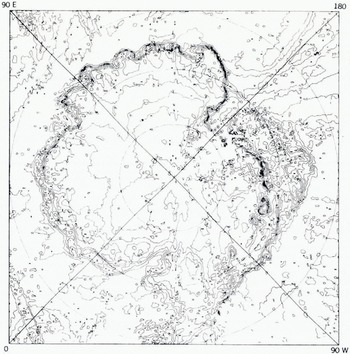
Fig. 16. Isoemissivity contours for a wavelength 1.55 cm on the Antarctic continent obtained by combining ESMR and THRI data obtained on.11 January 1973 (Figs. 12 and 13).

Combining the THIR and ESMR images over the continent, one can obtain contour maps illustrating the variation of emissivity of the continental ice sheet (Fig. 16). These contours result from a combination of two factors: (1) the physical temperature on the ice surface is lower at the higher elevations and (2) the crystal size distribution in the ice sheet differs in various geographical locations. It should be pointed out that what has been designated as emissivity is actually the ratio of the brightness temperatures at 1.55 cm and 11 μm. However, from computations based on a Mie scattering model it can be shown that the microwave radiation penetrates this ice sheet to a depth of the order of 10 wavelengths (Chang and Gloersen, unpublished). Therefore, the contours in Figure 16 only approximate the true emissivity since the THIR provides the temperature at the surface and the ESMR the average brightness temperature of about a 15 cm layer. On the basis of the Mie scattering model (Chang and Gloersen, unpublished), the contours in Figure 16 may reflect distributions in the average crystal size on the continent. This model predicts that the lowest emissivities will correspond to the largest average particle sizes, within the range of particles encountered on the continental ice sheet. The size of the particles does depend on the morphology of the ice in a particular region, which has some connection with the temperature range and proximity to open water in that region.

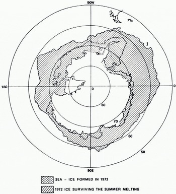
Fig. 17. Near-minimum and near-maximum Antarctic sea-ice boundaries for 1973 (10 February and 16 July).

The ESMR images can be used also to observe the variation of the sea-ice coverage with time. The approximate maximum and minimum sea-ice coverage in the South Pole region for 1973 as determined from the ESMR imagery is shown in Figure 17. The variation of ice concentration can also be inferred from these images, even when open water cannot be resolved by the ESMR, by using a linear interpolation between the emissivity of open water (0.4 at a wavelength of 1.55 cm) and that of first-year sea ice (0.95 or greater). The accuracy of this determination is better than ten percentage points; the error is largely due to the uncertainty of the actual temperature of the ice surface within a season. An example of an ice concentration map of Antarctica is shown in Figure 18. The ice concentration parameter is important not only for maritime interests but also for global weather models inasmuch as the heat transfer rate between the surface of the Earth and the atmosphere is strongly affected by the ice concentration.

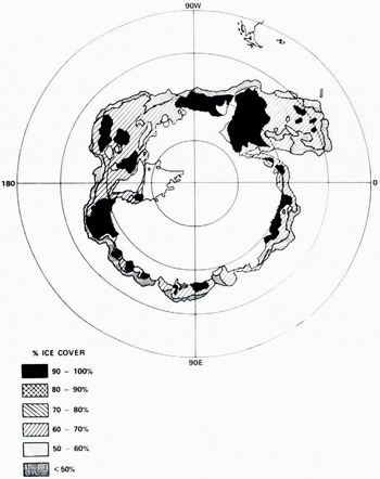
Fig. 18. Compactness of sea ice around Antarctica an 26 December1972.

The continental ice sheet on Greenland has remarkably different properties from that of Antarctica. In Figure 19 (pl. VIII), two ESMR images of Greenland are shown, one for the summertime and one for mid-winter. One can see a persistent brightness-temperature pattern also in this continental ice sheet. However, it should be noted that the brightness temperatures are the highest at high elevations, quite contrary to what is observed in Antarctica. The emissivity range on Greenland is illustrated in Figure 20, showing a range of emissivities similar to, but a spatial distribution completely different from, those observed in Antarctica. It is not surprising that the crystal size distribution in Greenland, as implied by the variation in emissivity, should be different from that of Antarctica because (1) the range of physical temperatures encountered includes the freezing point of" water in Greenland but not at all in Antarctica and (2) inland points in Greenland are considerably closer to open water than in Antarctica. That is to say, the metamorphosis of snow would be expected to be completely different in regions where thawing and freezing occur as opposed to regions where temperatures are always well below freezing.

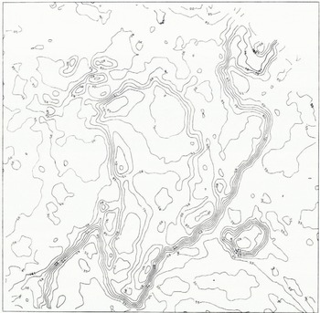
Fig. 20. Isoemissivity contours for a wavelength of 1.55 cm on Greenland obtained by combing ESMR and THIR data obtained on 11 January 1973.

Over the two-year observational period of the Nimbus-5, no significant changes have been observed in the emissivity contours in Greenland or Antarctica. On a long-term basis, changes in these patterns might be observed and could be indicative of slow climatic changes.

Seasonal changes in the continental ice sheet of Greenland, much stronger than those resulting from the seasonal Reference Chang and Gloersenchange in physical temperature, have been observed at the lower elevations where thawing and freezing take place. Edgerton and others (1971) have observed that wet snow results in a very much higher microwave brightness temperature than dry snow for snow of sufficient depth. This has been observed also from the ESMR on Nimbus 5 in both the multi-year portions of the Arctic Sea ice canopy and in the lower elevation regions of Greenland. It is possible that this phenomenon may be utilized to determine any changes in the snow-melt line in Greenland from one year to the next. An attempt has been made to estimate the snow-melt line on the continental ice sheet of Greenland based on the data available at the time of writing. The results are shown in Figure 21. The applicability of this technique must be confined presently to enormous glaciers such as the Greenland ice sheet because of the limited spatial resolution capabilities of the ESMR. However, when higher spatial resolution becomes available in the future, this technique may be extremely valuable in defining snow and firn lines on smaller temperate glaciers.

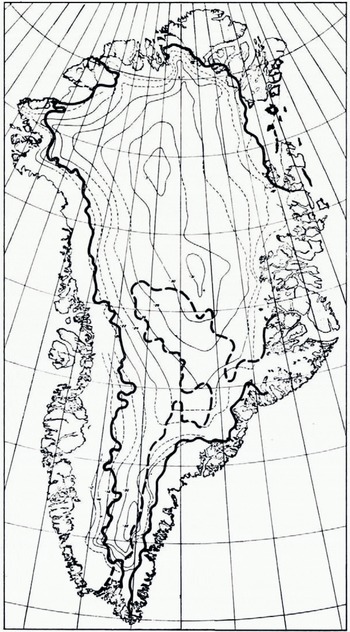
Fig. 21. The thick solid line is the summer melt line in the snow field covering the Greenland continental ice sheet as deduced from.Nimbus. 5 ESMR data obtained on 21 July 1973. The area to the east of the thick dashed line is that in which the highest microwave brightness temperatures were observed on 11 January 1973 (cf. Fig.19).

IV. Prospects For The Future

Continued improvements are envisioned for the future in terms of improved sensors and spacecraft systems with longer lifetimes. In the Earth resources survey area as it relates to snow and ice measurements, it is planned that RRTS-B will be launched in early 1975 or very shortly after ERTS-I becomes inoperative. ERTS-B will have the same spectral observation and spatial resolution capability as ERTS-I. An ERTS-C is planned for the 1977 time frame with an additional 10-11 μn thermal infrared observation capability.

As has been indicated in the preceding section, the microwave portion of the electromagnetic spectrum holds considerable potential for snow and ice mapping. In the immediate future another ESMR, this one operated at a wavelength of 0.8 cm and with both polarization components, is scheduled for launch on board Nimbus-F late in 1974- The next improvements in spacecraft instrumentation will be flown on the Nimbus-G in the form of a scanning multi-channel microwave radiometer (SMMR). Measurements will be acquired in five spectral bands with ten channels (because of dual polarization) in the wavelength region between 0.8 to 6 cm. The spatial resolution will again be modest and near 25 km for the shortest wavelength.

Future missions are being considered that will attempt improvements in spatial, temporal and spectral resolution. These missions include low-orbiting satellites with modular capability for including new instrumentation. This low-orbiting satellite series will be called Earth Observatory Satellites (EOS). Spatial resolutions in the visible region of the spectrum may be as high as torn. Larger observational swath widths would increase the frequency of coverage to 6-9 d with accompanying spatial resolutions 100 m or better. Attention will be given to the possibility of using synthetic aperture radar for providing high spatial resolution in the microwave wavelengths from 1-25 cm.

For snow and ice coverage, the next most interesting spacecraft concept beyond EOS would be the Space Shuttle Sortie-Spacelab concept with polar orbit capability being considered for the 1980’s. On the Spacelab, larger instruments of a developmental nature requiring more power, or operation and attendance by a scientist or technician, can be operated and tested for eventual long-term operation. For example large antennae associated with active or passive microwave systems could be tested. Relatively complex visible and infrared spectrometric equipment could also be developed in the Spacelab environments.

Another key facet of future spacecraft systems involves the development of data processing and analysis facilities that would handle data magnitudes as high as 250 megabits per second (Mb/s). It is clear that these data must in the future be optimally processed and delivered to user agencies so that these data products can be applied to resource management problems. To meet these general goals it is imperative that improved data-processing facilities be developed and communications improved between the developers of improved data-processing and dissemination facilities and the potential users of such information. Substantial efforts along these lines are being implemented within NASA in cooperation with major state and federal agencies.