Introduction
During the International Association of Scientific Hydrology symposium atObergurgl on variations of the regime of existing glaciers in September 1962 three of the authors of papers to be published shortly in this Journal met on the initiative of Hochstein to discuss their resistivity work and to agree that they would contribute their unpublished results to a joint paper on the subject, entitled “The electrical resistivity method used in glaciological work”. The idea was to cover different aspects of recent resistivity work on ice and to compare experience gained and results from various parts of the world. Additional authors could be found who were willing to contribute to the joint efforts. The individual contributions, which were collected by Röthlisberger, varied so much in scope and size that it looked more appropriate to keep them as a series of articles rather than to try to combine them in a single paper. Some obvious repetitions of statements by different authors have been deleted, however, and an adjustment of notations has been made.
By the electrical resistivity method we understand primarily geophysical prospecting techniques based on the measurement of the potential produced by a D.C. (or low frequency A.C.) current introduced into the ground.
Principle of Resistivity Soundings
Although it is not the purpose of this article to describe the resistivity method as such—geophysical textbooks may be consulted—a short note on the principles used seems appropriate for those readers who are not at all familiar with geoelectrical methods. The objective of geoelectrical surveys is to investigate the sub-surface by means of surface measurements. A standard technique consists of producing an electric current in the ground between two electrodes, the current electrodes, and to measure simultaneously the electric field between two different electrodes, the potential electrodes. With the 4-electrode method the variable contact quality at the current electrodes does not affect the result. Two electrode configurations are commonly used, both linear and symmetrical in respect to the centre (Fig. 1). In the Schlumberger configuration the separation l of the (inner) potential electrodes is small compared to the distance L between the (outer) current electrodes (l < L/5). In the Wenner configuration the total length of the line determined by the outer electrodes is divided into 3 equal sections of length a by the inner ones (l = a, L = 3a). Simple equations exist to compute the resistivity (electric resistance of a cylinder of unit cross-section and unit length) in case of the homogeneous isotropic half-space. If the same equations are used when the half-space is not homogeneous the result is called the “apparent resistivity”, ρ a. The equations read:

where ΔV is the potential difference and I the current. The Wenner configuration with an additional electrode at the centre is called the Lee configuration. Potentials are measured between this central electrode and both Wenner electrodes, one at a time. Differences between the two measurements are indicative of surface inhomogeneity or a sloping interface. In many cases it is more economical to use asymmetrical electrode configurations in place of the symmetrical ones. The equations for ρ a are simply changed by a factor of 2 when three electrodes are arranged as in the standard Schlumberger or Wenner configuration and one current electrode is permanently placed at infinity, i.e. at a suitable place very far away. Only one or two electrodes have then to be moved at a time; however, the effect of local inhomogeneities is generally more disturbing than with the symmetrical configurations.

Fig. 1 Common electrode configurations
For interpretation the case of horizontal layers is of prime importance. Then, for a given sequence of layers, the apparent resistivity ρ a is only a function of the electrode spacing; the larger the electrode separation, the deeper the current penetrates, and the larger the influence of deeper layers becomes. Theoretical curves (or master curves) have been published for selected combinations of layers (CGG, 1955; Reference Mooney and WetzelMooney and Wetzel, 1956). These curves are plotted non-dimensionally on double logarithmic paper (for unit thickness and unit resistivity of one of the layers). By matching a theoretical curve with a measured one the various thicknesses and resistivities of the layers are obtained; the proportionality factors are given by the horizontal and vertical shift necessary to match the curves. For a given curve an infinite number of solutions exists if an infinite number of layers is introduced. With a finite number of layers the solution is theoretically unique. However, because of the limited accuracy of the measurements, there is ambiguity even with only three layers present. A good fit of a curve therefore does not necessarily mean that the result is correct. For a good interpretation of geoelectrical measurements it is very important to have some knowledge of the layering and the resistivities. Most of this knowledge comes from experience and it is part of the objective of this series of papers to make experience available to future workers in this field.
Specific Problems With Resistivity Measurements on Glaciers
Although the principle of the measurements is the same in the glaciological as in the general geophysical applications there are some methodological specialities worth mentioning. Glacier ice is a material with a very high resistivity, and therefore extremely large resistivity ratios are sometimes encountered between conductive surface layers and the ice as well as between ice and bedrock. For such cases master curves had not been numerous until Reference CagniardCagniard (1959) improved the situation by giving a set of curves for a highly conductive thin surface layer on an infinite plate with much higher resistivity followed by an ideal conductor, a sequence of layers typical for temperate glaciers. This is a particular three-layer case, which is normalized by setting h 2 = ρ 2 = 1, h 3 = ∞, ρ 3 = 0, and using α = h 1 ρ 2/h 2 ρ 1 as a curve parameter, where h 1, h 2, h 3 are thicknesses and ρ 1, ρ 2, ρ 3 resistivities of successive layers. Cagniard has published a total of 14 curves for parameters between 0.01 and 100. For parameters below 1 the curves differ from each other in shape; the smaller the parameter the flatter the peak, and a fairly unequivocal superposition of measured data and theoretical curve is possible. Curves with higher parameters show almost identical, narrower peaks. They differ mainly by their position on the diagram, and the evaluation of that type of curve is ambiguous over a wide range of ice thicknesses and resistivities. The curves have a common evolute, however. If one of the variables, ice thickness h 2 or resistivity ρ 2 are known, the other variable as well as the appropriate parameter α can be found by sliding the measured curve along the evolute to the position determined by the given thickness or resistivity, whichever is known. A prerequisite for this procedure is that the bulk of the glacier is electrically homogeneous. For parameters α between 1 and 100 the evolute is only slightly curved and slopes at close to 45°, which means that ice thickness and resistivity are about reciprocal, i.e. assuming twice (or n-times) the resistivity only half the ice thickness (or 1/n of it) will be obtained.
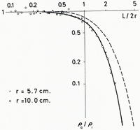
The usual master curves do not take the trough-shape of valley glaciers into account. In order to have some idea of its effect, we have experimented with small-scale models consisting of semi-circular metal channels filled with water. Satisfactory results could be obtained with A.C. measurements only, whereas with D.C. the polarization effects proved to be very bothersome. The potential was measured at the water surface along the axis of the semicircular cylinder, while one of the two current leads was connected to a small electrode in the axis, representing a point source, and the other to the metallic trough. The potential values as a function of distance from the point source were used to compute the data for a standard master curve for the Schlumberger configuration along the axis of a semi-circular cylinder of radius r = 1 and resistivity ρ 1 = 1, imbedded in a substratum of resistivity ρ 2 = 0. The results are plotted in Figure 2, where a good agreement between the results from two different sizes of channels can be noted. The master curve for an infinite plate of thickness h = r = 1 and resistivity ρ 1 = 1 resting on an infinitely conductive substratum (ρ 2 = 0) is also plotted. From the horizontal shift of the two curves it can be seen that the true radius r of a semicircular bed is by about 20–35 per cent larger than the depth h obtained with the master curve for a plate. This is the correction one has to apply when using Cagniard curves with small parameters α; for increasing parameters α it may be suspected that the correction should become larger, but how much has not yet been investigated by us. It is still an open question what correction is needed when the ratio ρ 1/ρ 2 is not large.

Fig. 2 Empirical results for resistivity soundings with Schlumberger configuration in the axis of a semi-circular channel of radius r in infinitely conductive material. Solid line = empirical ρa curve; dashed line = theoretical curve for infinite plate of thickness h = r, Cagniard parameter α = 0 This figure is reproduced to such a size that it will superpose on log–log paper of the size customarily used in resistivity work (base 62.5 mm.). Resistivity diagrams in the following papers of this series have had to be reduced to one half of this size
The high resistivity of the ice is equally important for the instrumentation. Standard geoelectrical equipment cannot be used because the impedance of the potential measuring circuit is too low. Electronic electrometers have to be applied instead to measure the potentials. The Keithley instruments have proved adequate and very reliable under all sorts of field conditions. Using dry cell batteries of 100 to 1000 V., currents of the order of 0.5 to 1 mA. are usually obtained, which are easy to measure. Potentials from 10 mV. to several volts are then observed. High standards are not only necessary for the electrometer, but also for the insulation of cables and connectors, and frequent insulation control is recommendable. Reference CarpenterCarpenter (1955) has described a simple method of leakage control for the Wenner configuration based on an exchange of current and potential electrodes, but disconnecting the current circuit at one (or both) current electrodes may prove to be even simpler. Communication between the operator at the centre and the aides at the ends of the spread may be difficult, however, because of the long electrode separations needed in glacier soundings. Reference GreenhouseGreenhouse (unpublished) has suggested ammeters hooked in between the leads and the current electrodes as a simple means to keep the aides informed on the progress of the measurements and to give coded instructions.
Metal rods or wire nets are used as current electrodes, while stainless steel or copper rods, or copper–copper sulphate porous pots (non-polarizing electrodes) serve as potential electrodes. To lower the contact resistance at the current electrodes salt, graphite and anti-freeze have been used. On cold glaciers and ice caps anti-freeze has the advantage that the contact resistance stays approximately constant during the measurements, which is not true for salt. The non-polarizing electrodes make good contact at air temperatures slightly below freezing or higher. At lower temperatures they start to freeze up and become very troublesome.
Because of the high-impedance circuits it becomes difficult to work in damp weather. With high winds and drifting snow measurements become impossible, because of rapidly fluctuating potentials of the same order of magnitude as the effects under observation probably caused by moving charged air masses and the friction of snow particles. Some slowly variable earth potentials are also present. It is therefore standard practice to take simultaneous readings of the current and potential very shortly (1–10 sec.) after closing the circuit, to break the circuit again and to check if the original potential has not changed. Measurements are then made with reversed polarity. A common observation is that the currentwill decrease with time at one polarity and remain stable at the other, while the apparent resistivity remains approximately the same. On other occasions (especially in cold ice) more or less pronounced polarizations have been observed, however. Strong A.C. fields have occasionally affected the measurements with the Keithley electrometer, a difficulty easily overcome by shunting the instrument with a high-impedance capacitor.
Glaciological Applications
We are dealing here with the glaciological applications of the resistivity method only in so far as glaciers or glacial ice are concerned. We shall therefore not discuss the use of the method for the investigation of permafrost, which has a long-standing history, and we shall not discuss for instance its use on sea ice. In this sense resistivity surveys have primarily been proposed as a sounding technique to measure the thickness of glaciers. The great advantage of the method is the relatively cheap and light-weight equipment and the smallness of the field party (a minimum of 3 men). Where an approximate figure for an average ice thickness over a certain area is sufficient, successful resistivity soundings could replace the much costlier seismic soundings.Footnote * Various efforts have therefore been made to develop the method, and it is one objective of this series of articles to discuss its potential as a sounding technique.
For interpretation the resistivity of the ice is a decisive factor. The early investigations showed soon that resistivity is by no means a constant for all glaciers, and may even vary considerably in one particular ice body. These variations make sounding difficult, but are interesting in themselves. At the present stage of our knowledge it even appears that the material property, resistivity, may be the more important subject of an investigation than depth, and part of the series of papers deals with the material property side of the work. As far as the explanation of resistivity variations in glaciers is concerned, it is not easy to apply the extensive work of physicists on conductivity of ice (mainly carried out on single artificial ice crystals) because there are too many incompletely known parameters. These problems will be discussed in a future article by Andrieux.
Apart from its application as a geophysical prospecting method, resistivity measurements can serve to locate markers (electrodes) placed in the ice or snow of a glacier. Reference BorovinskiyBorovinskiy (1958), for instance, had used this technique for movement studies. Different work of this type is in progress near Jungfraujoch, where we are using a blank copper wire to mark a complete section across a firn field for accumulation studies. It has been possible to locate the position of a wire at 4 m. depth with an accuracy of about 10 cm., but it is 100 early to give a final appraisal of the method. Weather-dependence is certainly a great drawback.
Former Work
Reference RomanRoman (1938) was probably first to report on successful experiments with electrical resistivity sounding techniques on snow (by modified standard equipment) and to propose the use of the method on glaciers. But only in recent years has interest in doing so really awakened, and after an initial trial with modern equipment by a French group in 1956 (Reference Queille-Lefèvre and LefèvreQueille-Lefèvre and others, 1957) field parties of various countries operated independently on a number of glaciers.
In an internal report, Reference VögtliVögtli (unpublished [a]) described his first measurements, which were carried out near the snout of Steingletscher (Switzerland) using a Keithley electrometer (model 200 B). Besides proving that the chosen instrument was fully adequate for field work, promising sounding results were obtained. By means of the master curves of CGG (1955) and Reference Mooney and WetzelMooney and Wetzel (1956) depths of 50 m. and 73 m. were found for two profiles at right angles based on resistivities of 10 to 14 MΩ.m. for ice (0.8–0.9 MΩ.m. for snow). A French group (Reference Queille-Lefèvre and LefèvreQueille-Lefèvre and others, 1959) carried out resistivity soundings on Glacier de St. Sorlin (France) in the same year. They too stressed the feasibility of resistivity soundings. Analysing their data with the theoretical curves prepared by Reference CagniardCagniard (1959) especially for this particular project, they obtained an ice thickness of 52.8 m. with a resistivity of 87.5 MΩ.m., but noticed a fair amount of ambiguity, actually obtaining a large range of thickness between 27.5 m. and 79.4 m. with respective extreme resistivity values of 170 MΩ.m. and 59 MΩ.m. They pointed out that the method would be more promising when applied under more favourable surface conditions, i.e. with a “dry” surface. Reference BorovinskiyBorovinskiy (1958) too gave a very favourable report on the applicability of resistivity soundings, working 1957/58 on Lednik Tuyuksu (Soviet Central Asia). He made use of the method to distinguish between different types of ice, like a surface layer 15 m. thick with lower resistivity, investigated moraines, some containing ice masses, and developed a technique to survey ice flow at some depth by placing an electrode in a drill hole. He omitted to give values of ice resistivities, but Reference VögtliVögtli (unpublished [b]), in another internal report, listed values of 75 MΩ.m. and 17 MΩ.m. at two places in the ice tunnel at Jungfraujoch (ice temperature −2.6° ±1° C.). Reference Keller and FrischknechtKeller and Frischknecht (1960) working with an asymmetrical electrode arrangement with a single moving electrode and pulsed D. C. current of 0.1 to 3 sec. duration on Athabasca Glacier (Canada) in 1959 gave further evidence of high resistivities in temperate glacier ice (3.5 to 22 MΩ.m.), but found evidence of considerable inhomogeneity. (The large scatter of their measurements was probably partly due to the method used.) They expressed the opinion that resistivity soundings are limited in accuracy but give interesting information on the ice as a material. (For determining depth and character of the substratum an electromagnetic method tried at the same time was found to be more adequate.) Reference BorovinskiyBorovinskiy (1961) described techniques using asymmetrical electrode configurations and combinations of such with symmetrical ones which enabled him to solve cases of lateral inhomogeneity and to take the shape of the bed into account.
In the meantime a striking phenomenon had been observed, that the resistivities in the cold ice of polar glaciers were smaller by orders of magnitude than those of temperate glaciers. Reference Meyer and RöthlisbergerMeyer and Röthlisberger (1962) observed resistivities of only 0.1 MΩ.m. for ice at approximately −12° C. in the neighbourhood of Thule Air Base, Greenland. Although they had seismic control of some of the ice thicknesses, a satisfactory interpretation of their soundings was not possible because of the presence of a high resistivity layer of unknown thickness and origin at the base of the ice. Further resistivities were measured near Camp Century on the névé of the Greenland Ice Sheet 200 km. from the coast, where the mean annual temperature is estimated at −24° C.; a decrease from 0.35 MΩ.m. near the surface to about 0.1 MΩ.m. at a depth of roughly 50 m. was observed, the resistivity still decreasing with depth. In the centre of Greenland Reference HochsteinHochstein (1965) found in 1959 a similar decrease of resistivity with depth and also low resistivity at still colder temperatures and down to considerable depth. Vögtli and Greenhouse (in Reference ApollonioApollonio and others, 1961) confirmed the low resistivity of cold ice by their measurements on Devon Island. They found in general the sequence of low resistivity ice (0.05–0.1 MΩ.m.) and high resistivity bedrock (1 MΩ.m.) which was favourable for depth soundings. Details of this work are given in one of the present articles (Reference VögtliVögtli, 1967).
Reference ØstremØstrem (1959, Reference Østrem1962, Reference Østrem1964) has used the resistivity method quite extensively for a different glaciological problem from depth soundings, namely for locating ice cores in moraines. The method proved very well suited for this type of work. The method has also been useful since 1956 in engineering exploration for hydro-electric projects in Switzerland in connection with buried ice (personal communication from Dr. W. Fisch, Kilchberg, Switzerland).
Recently the glaciological applications of the resistivity methods have been treated by Reference BorovinskiyBorovinskiy (1963). Reference GreenhouseGreenhouse (unpublished) and Reference AndrieuxAndrieux (unpublished) have presented their investigations on the subject as doctoral theses which both contain many details that cannot be dealt with here. Reference Chaillou and VallonChaillou and Vallon (1964) present some results of resistivity measurements on an Alpine valley glacier (resistivity 50–70 MΩ.m.) and on a névé field.
Acknowledgements
Thanks are due to Prof. G. Schnitter and Ing. P. Kasser for their authorization to carry out the resistivity work as part of the programme of the Section of Hydrology and Glaciology, to Prof. H. Grubinger for letting me use the facilities at the Kulturtechnische Institut for the model studies, to Dr. U. Schryber of the Physics Department for his instructions in the use of the various pieces of equipment, and to Mr. P. Föhn for carrying out the measurements. The author wants to apologize to those authors of articles of the series whose manuscripts have remained an unduly long time on his desk, and he wants to thank those who have contributed with their suggestions to his paper.