Article

Sustainability Concept in Decision-Making: Carbon Tax Consideration for Joint Product Mix Decision

1
Department of Business Administration, National Central University, No. 300, Jhongda Rd., Jhongli, Taoyuan 32001, Taiwan
2
Department of Business Administration, Fuzhou University of International Studies and Trade, Fuzhou 350202, Fujian, China
*
Author to whom correspondence should be addressed.
Sustainability 2016, 8(12), 1232; https://doi.org/10.3390/su8121232
Submission received: 22 September 2016 / Revised: 15 November 2016 / Accepted: 17 November 2016 / Published: 26 November 2016
(This article belongs to the Section Economic and Business Aspects of Sustainability)

Abstract

:
Carbon emissions are receiving greater scrutiny in many countries due to international forces to reduce anthropogenic global climate change. Carbon taxation is one of the most common carbon emission regulation policies, and companies must incorporate it into their production and pricing decisions. Activity-based costing (ABC) and the theory of constraints (TOC) have been applied to solve product mix problems; however, a challenging aspect of the product mix problem involves evaluating joint manufactured products, while reducing carbon emissions and environmental pollution to fulfill social responsibility. The aim of this paper is to apply ABC and TOC to analyze green product mix decision-making for joint products using a mathematical programming model and the joint production data of pharmaceutical industry companies for the processing of active pharmaceutical ingredients (APIs) in drugs for medical use. This paper illustrates that the time-driven ABC model leads to optimal joint product mix decisions and performs sensitivity analysis to study how the optimal solution will change with the carbon tax. Our findings provide insight into ‘sustainability decisions’ and are beneficial in terms of environmental management in a competitive pharmaceutical industry.

1. Introduction

There are many companies using the same raw materials in continuous production processing and that use the same processes to output joint products of two or more different characteristics or uses, such as the petroleum industry, chemical industry, steel industry and pharmaceutical industry. Such split-off joint products may be sold immediately or be further processed before being sold. The costs prior to the split-off point are joint costs, which are the main costs required for the production of various products; while the costs of additional processing procedures of some joint products are separable costs. After the split-off point, whether to sell or continue to process is subject to the marginal contribution of further processing, capacity resource constraints, market demands and other factors [1,2,3].
The Paris Agreement was signed by 195 nations on the 12 December 2015 to strengthen the global response to the threat of environmental climate change, which was in the context of sustainable development and efforts to eradicate poverty, after the 1992 United Nations Framework Convention on Climate Change (UNFCC) and the 1997 Kyoto Protocol. In Article 2 of the Paris Agreement, the increase in the global average temperature is anticipated to be held to well below 2 °C above pre-industrial levels, and efforts are pursued to limit the temperature increase to 1.5 °C above pre-industrial levels (United Nations, 2015). Carbon emissions are receiving greater scrutiny in many countries due to international forces to reduce anthropogenic global climate change. The carbon tax constraint is one of the most common carbon emission regulation policies that companies must incorporate into their production and pricing decisions. Activity-based costing (ABC) and the theory of constraints (TOC) have been applied to solve product mix problems; however, a challenging aspect of the product mix problem involves evaluating joint manufactured products, while reducing carbon emissions and environmental pollution to fulfill social responsibility. Many scholars have proposed using TOC, ABC and linear programming (LP) to solve the product mix problem and obtain the optimized results [1,4,5,6,7,8]. TOC assumes how companies make the most efficient use of resources under existing resources; thus, the model is suitable for short-term decision-making. ABC assumes that all resources can be allocated according to activities, which are then allocated to cost objectives based on the activity drivers. Furthermore, it enables enterprises to recognize value-added and non-value-added activities in order to improve the use of resources; thus, the model is suitable for long-term decision-making.
The conventional ABC model contains a large number of activities. With the changing growth scales of business operations or production processes, in order to measure the different resources used, as well as the costs attributable to operations and production, new activities must be constantly added, which renders production more complex. In addition, many complex cost drivers require the subjective estimates of staff; thus, allocation percentages are also subjectively set by staff, which may lead to various product mix decision-making results due to subjective differences. If the conventional ABC method does not fully use time drivers, it may overlook potential unused capacities regardless of whether resources are fully used, and they will be attributable to the product cost [9]. To achieve higher accuracy, activities must be piecemealed; however, more piecemeal activities can easily create too large a database. In addition, when there are multiple constraints and integer solution assumptions in TOC, there may not be an optimal solution [10,11]. Although Fredendall and Lea [12] suggested that the optimal solution can be obtained by repeated solution-finding iterations, such an approach will become more complex in the face of added constraints; thus, enterprises will gradually pay more than the exact cost in order to obtain more accurate cost information for consideration.
Therefore, in 2004, Kaplan and Anderson proposed time-driven activity-based costing (TDABC), which is mainly based on the total time of an activity as a cost allocation basis. TDABC applies time drivers directly from the resource to the cost objective, omits the time-consuming and subjective estimates of the first stage and does not require an estimated time percentage investment for each activity at the second stage. Compared to the conventional ABC model, it can better reflect the complex realities and time differences of different activities [13,14,15]. In addition, in the conventional ABC model, the costs of activity centers are attributed to cost objectives without considering the capacity use of the activity centers. TDABC measures resources used according to output, where only the costs of use (time) is attributed to the cost objective; thus, enterprises can clearly recognize whether the resources of each activity center have been adequately used [16]. With limited resources, companies pursue long-term profits, while reducing environmental pollution, to fulfill social responsibility [17,18,19]. Therefore, joint product mix decision-making should consider the marginal contribution of continuous processing, capacity resource constraints, market demand and other factors [1,3,4], as well as reducing pollution emissions [20]. As TDABC is a new management tool, previous relevant research literature on TDABC is relatively limited [14,16,21].
The main purpose of this research is to use an actual case of the pharmaceutical industry, which uses the relevant information regarding the activities of active pharmaceutical ingredients (APIs) processing to the drugs available for medical use. In addition to considering continuous processing, capacity resource constraints, market demand and other factors, the process of reducing pollution is considered. By establishing TOC, ABC and TDABC joint product mix models and using the mixed-integer programming (MIP) method to determine the optimal joint product mix, this paper analyzes the resources used and determines whether joint products after the split-off point should be directly sold or be further processed before being sold in order to provide reference for managers in green decision-making. The remainder of this paper is organized into four sections. Section 2 details the literature regarding the concepts of the carbon tax, TOC, ABC and TDABC in the pharmaceutical industry. This study develops the TDABC model for joint product decisions in Section 3. A numerical example is used to demonstrate how to solve these models with MIP through sensitivity analysis and under the possible constant carbon tax, to lead to an optimal solution in Section 4. Finally, this study presents the conclusions in Section 5.

2. Literature Review

2.1. Carbon Tax

Carbon taxes are important and aim to reduce the carbon emissions that are directly related to the carbon content of fuels. In the green building industry, the management of carbon emissions from green building projects contributes to the acquisition of accurate building cost information and reduces the environmental impact of these projects. The levying of carbon taxes also increases building costs for construction companies. With the heightened awareness of corporate social responsibility (CSR), construction companies must consider carbon emission costs to help accurately predict building costs and reduce the project’s overall impact on the environment [22]. Therefore, carbon taxes are levied according to the emission price per ton. In fact, carbon taxes are an important policy tool for environmental protection, as it prompts companies to pursue optimal environmental management under tax considerations.
Currently, carbon taxes are assessed differently from country to country due to variances in environmental policies, and companies must incorporate carbon taxes in their production and pricing decisions. This study intends to explore the effects of carbon tax levy methods on joint product mix decisions. Figure 1 presents the minimum threshold for carbon taxes (i.e., no taxes below the thresholds). Figure 2 shows the levy of carbon taxes at a specific tax rate in the absence of tax thresholds. Figure 1 illustrates the fixed tax rate schedule once the threshold has been surpassed. Figure 2 shows the full progressive tax rates once the threshold has been reached. A higher rate is imposed on higher carbon contents, and all carbon content levels are accompanied by corresponding progressive rates. While the full progressive tax system reports better results in carbon reductions, the extra progressive tax system seems a more reasonable approach, as the latter allows for different rates at different carbon levels and can create a meaningful impact in carbon reductions.

2.2. Concepts of ABC and TDABC

Kaplan and Cooper first proposed ABC in 1988, which was mainly to overcome the distorted situation under the conventional cost accounting system and cost of subsidies [23]. The disadvantage of the conventional cost system is the assumption that the cost allocation basis of manufacturing costs is quantity related. In fact, not all manufacturing costs and quantities are related; therefore, the conventional cost system may cause cost distortions, leading managers to make erroneous pricing decisions. When the proportion of enterprise manufacturing costs and the degree of product diversification are higher, the possibility of cost distortion through the conventional cost accounting system is higher. The adoption of the ABC method can provide enterprises with value-added information and non-value-added costs in a systematic manner, in order to generate a more precise and efficient performance with sustainable consciousness [24].
ABC uses a two-stage cost allocation method, which considers resource drivers and activity drivers. At the first stage, the correlation between resources and activity costs is analyzed by planning the resources into a number of activity centers. At the second stage, the appropriate cost drivers are determined according to different activity levels (e.g., unit-level, batch-level, product-level, facility-level), in order to summarize cost databases before attributing costs to cost objectives, thus obtaining reliable cost allocation information [9,25]. Kaplan and Cooper argued that ABC emphasizes the relationship between the activities and the consumption of resources; therefore, it can provide product decision-making information and help managers with decisions regarding product design, pricing, product mix, marketing and process improvement [26].
However, ABC assumes that each activity uses a single cost driver, namely all of the orders and activities of a certain type of product are the same; in this hypothesis, the processing time is the same. In fact, each activity may have more than one cost driver, for example order processing costs are not only related to the number of orders processed, but are also related to order quantity; therefore, the activity can be divided into two parts. However, this approach will lead to increased activities and difficulty in estimating the actual production capacity. Therefore, Kaplan and Anderson (2004, 2013) [27,28] developed TDABC to overcome this difficulty. TDABC uses activity time as the basis for cost allocation. Parameters for estimation by this approach include: the unit time cost, which is generally the division of the total cost of a department by the total working hours of the staff in the department; the time consumed for each activity, namely multiplication of the activity unit time and the corresponding activity to obtain the total costs of the activity [27]. These parameters do not require formal investigation and can be obtained by direct observation or staff interviews. Through observation, this paper determines how long it takes to complete an activity. Moreover, these two parameters can completely replace the previous two-stage cost allocation process of resources to the cost objective and simplify cost steps to reduce the risk of the non-objective estimation of drivers due to the number of cost allocations during the computation process [28,29].
Another feature of TDABC is the use of a time equation to express the complexity of the actual operation, as follows:
Y = β 0 + β 1 χ 1 + β 2 χ 2 + + β i χ j
where β 0 is the standard time of basic activities; β 1 ( i = 1, 2, …, n) is the estimated time for additional activities; χ j ( j = 1, 2, …, n) is the events of the additional activities, which can be a continuous variable, an intermittent variable or a dummy variable [28]. Pernot et al. (2007) pointed out that TDABC can clearly demonstrate how long it takes to complete a certain activity, which can increase transparency, as compared to the conventional cost accounting system or ABC [13,30]. Varila et al. (2007) argued that it is more suitable to use time drivers rather than activity drivers if the resource consumption and time are directly correlated. By case study, they found that complex activities cannot be measured by ABC’s single activity driver; therefore, they proposed using bar codes, radio frequency identification (RFID) and other automatic data collection (ADC) methods in order to improve the disadvantages, including manual collection time, costs and the impossibility of immediate updating [31]. Kaplan and Norton (2008) mentioned that TDABC can predict the required production capacity according to future sales targets and is mainly used to determine required production capacity according to previous experience. When productivity or processes are improved, it can easily update time equations, estimate the resources required to determine the number of required staff and equipment and predict future profits, in order to understand profitability through the preparation of expected profit and loss accounts [32,33].

2.3. Applying TOC and ABC to Product Mix Decision-Making

In recent years, sustainable development strategies for enterprises have become an important global issue, as it is very important to create sustainable competitive advantages for enterprises. Enterprises must consider the shortage of resources, time, personnel and money, by selecting the optimal management systems under resource constraints, know how to cope with the interdependencies among various criteria, deal with constraints on resources and demonstrate how to select management systems for phase implementation [34].
TOC, as proposed by Goldratt and Cox, is mainly to resolve short-term product mix and processing bottleneck resource problems, as it improves the method of the conventional cost accounting system, which hinders the effective output of a company, and argues that all organizations have restrictions that will affect the operation of the entire organization. Therefore, bottlenecks can be identified by TOC, which improves such limitations [35].
Plenert argued that TOC limits apply only to a single resource constraint, and when multiple resource constraints exist, the decided product mix may cause other non-limiting resources beyond the capacity load, which is commonly referred to as bottleneck shiftiness. Finally, the obtained product mix is not the optimal product mix, and such a limit can be overcome by integer linear programming (ILP) [10]. In fact, Fredendall and Lea (1997) suggested that TOC also applies to multiple constraints and can similarly obtain the optimal solution by repeated solution searches [12]. Aryanezhad and Komijan (2004) argued that the algorithm for repeated solution findings, as proposed by Fredendall and Lea (1997), requires more time; therefore, they proposed an algorithm similar to multi-objective decision-making in order to improve the single objective algorithm for repeated solution finding [36]. Kirche and Srivastava (2005) used ABC and MIP to find solutions to problems and suggested that ABC can increase profits and reduce inventory levels more effectively than TOC [7]. Kee discussed product mix in the case of resource flexibility, namely, materials with quantity discounts and labor productivity that can cope with insufficient capacity through overtime or rental equipment [37]. Gong and Hu (2008) developed a product mix flexibility model that considers labor flexibility and machine flexibility in uncertain environments, which can help decision makers to obtain the optimal configuration for product mix [8], found that the bottleneck factors determine the level of product mix flexibility and that bottleneck improvements make a better contribution to non-bottleneck improvements.

2.4. The Pharmaceutical Industry Joint Product Mix Decision-Making

In the pharmaceutical industry, the joint production process from APIs’ processing to drugs for medical use is very complex. By case study combined with TOC through accurate cost analysis, it can assist managers in joint product mix decision-making analysis. Regarding joint products’ optimal product mix decision-making, Hartley (1971) discussed the further processing or direct sale of joint products after the split-off point by using mathematical equations to determine how many of the joint products should be sold and how many require further processing after the split-off point [3]. Tsai et al. (2007) used the algorithm to analyze the optimal joint products mix decision-making of TOC [38]. Tsai and Lai (2007) took further advantage of mathematical planning, as combined with TOC through accurate cost analysis, to design an activity-based cost decision-making model that enables companies to maintain a balance between internal production and outsourcing [39]. Tehrani and Michelot (2009) used the actual case of a refinery to discuss the effective use of the LP mathematical model for allocation regarding joint costs [40,41]. Tsai et al. (2013) combined the activity costing system and TOC to propose using the LP mathematical model to analyze product mix optimization decision-making in the case of a green manufacturing system, while considering continuous improvements of scale and other factors [20].
As TDABC is a new management tool, the relevant research literature is relatively limited. This paper uses information relating to the process of the pharmaceutical industry from APIs to drugs for medical use, in order to establish TOC, ABC and TDABC joint product mix models. The MIP method is used to solve the problem of the optimal joint products mix, analyze the resources used and determine the further processing or resale of the joint products after the split-off point. The findings can provide reference for managers in decision-making.

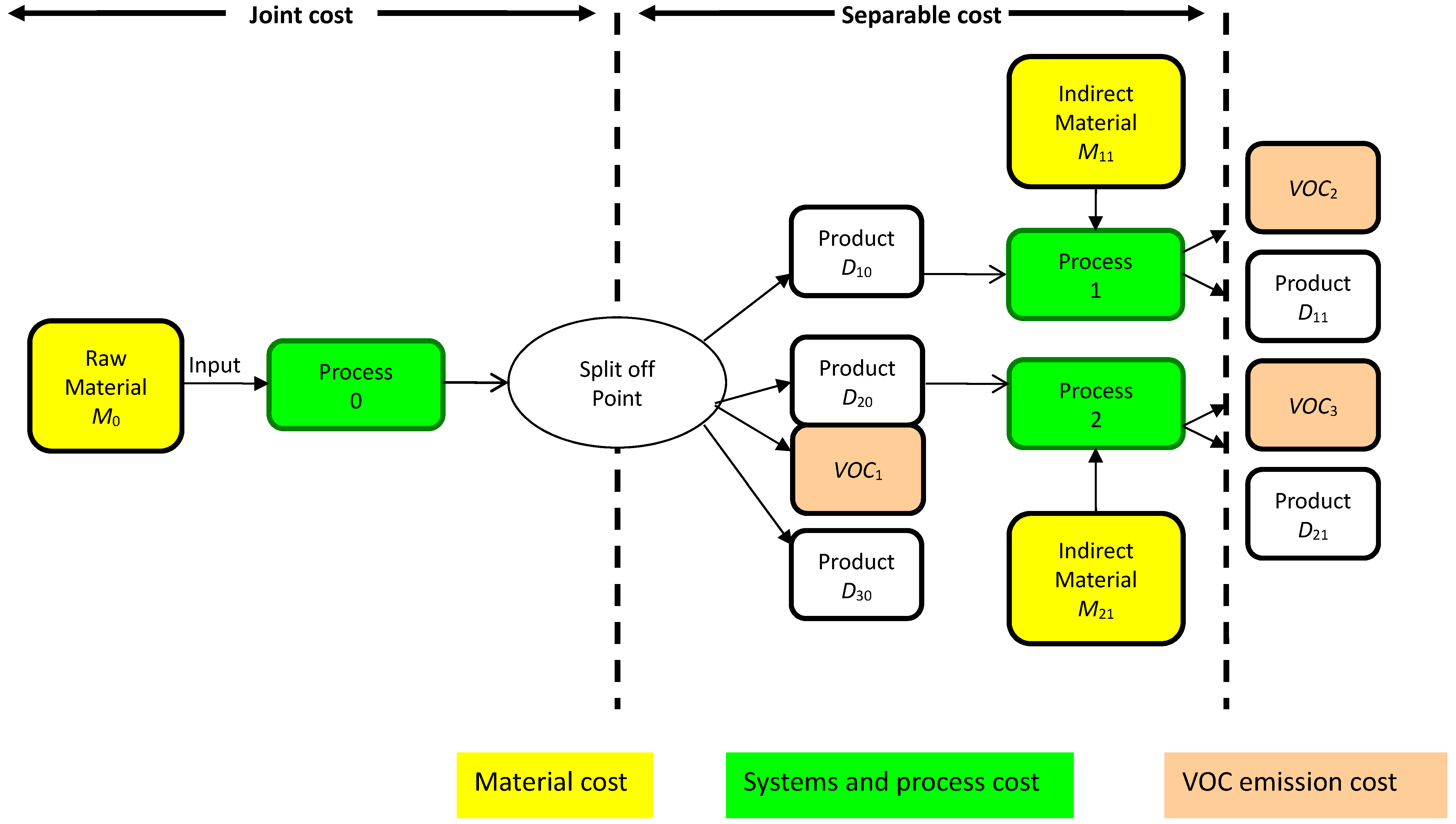
3. Models for Joint Product Mix

Most previous studies proposed using TOC or ABC to solve product mix problems. This paper establishes TOC, TDABC and ABC joint product mix models and sensitivity analysis with the carbon tax. In order to maximize total profit under various resource constraints, the case company, which produces joint products, must assess the desirability of further processing of such joint products after the split-off point. Three decision models for joint products mix are presented in this paper, and a simplified case is used to demonstrate the process of decision-making and profit analysis under each model. It is assumed that the case company can plan according to the current production capacity, but cannot increase the production capacity of activities in the case of insufficient production capacity. The mixed integer programming (MIP) method is used to obtain the optimal joint product mix, analyze the resources used and determine whether joint products should be directly sold or be further processed after the split-off point, and the models are compared in order to determine the model that can maximize profits.

3.1. Notations

3.1.1. Decision Variables

The following are the notations of the decision variables used in this paper:
  • π  is the company’s profit;
  • η 0  is the quantity of material APIs for the production of the joint product;
  • η i 0  is the production quantity of joint product D i 0 at the split-off point;
  • η i 1  is the quantity of joint product D i 1 processed further in a separate process after the split-off point;
  • ω i  is the units of D i 0 product for each unit of joint production (coefficient of the joint production);
  • g i  is the units of D i 1 products produced by processing each unit of D i 0 products after the split-off point (coefficient of processing production after the split-off point);
  • β i 0  is the batches of joint products;
  • β i 1  is the batches of products processed after the split-off point;
  • δ i 0  is the quantity of a shipment of joint product D i 0 ;
  • δ i 1  is the quantity of a shipment of product D i 1 processed further in a separate process after the split-off point;
  • R i 0  is the demand for joint product D i 0 ;
  • R i 1  is the demand of product D i 1 after the split-off point;
  • σ 1  is the tableting department labor/hour production capacity;
  • σ m  is the production capacity of tableting machine operating hours;
  • σ 0  is the order processing and tableting control department production capacity;
  • σ δ  is the shipping department production capacity;
  • σ τ  is the pharmaceutical inspection capacity;
  • σ υ  is the VOCs’ disposal capacity;
  • τ i 0  is a zero, one variable; if joint product D i 0 is not produced, it is zero; otherwise, it is one;
  • τ i 1  is a zero, one variable; if product D i 1 is processed further in a separate process, but is not produced after the split-off point, it is zero; otherwise, it is one.

3.1.2. Parameters

The following notations of the parameters are used in this paper:
  • X i 0  is the unit price of joint product D i 0 at the split-off point;
  • X i 1  is the unit price of joint product D i 1 processed further in a separate process after the split-off point;
  • MA0 is the unit price of material APIs for the production of the joint product;
  • MAi1 is the unit price of material APIs for the further processing of the joint products;
  • F C  is the marketing, plant guard and management costs;
  • t l i 0  is the direct labor hours demanded for the production of joint product D i 0 ;
  • t l i 1  is the direct labor hours demanded for the production of product D i 1 processed further in a separate process after the split-off point;
  • t m i 0  is the hours for the operation of the tableting machine for the production of joint product D i 0 ;
  • t m i 1  is the hours required for the processing and production of product D i 1 after the split-off point;
  • t b i 0  is the time to initiate the tableting machine for joint product D i 0 ;
  • t b i 1  is the time to initiate the tableting machine for joint product D i 1 processed further in a separate process after the split-off point;
  • t o i 0  is the time of order processing of joint product D i 0 ;
  • t o i 1  is the time of order processing of joint product D i 1 processed further in a separate process after the split-off point;
  • t c i 0  is the time to shift each batch of APIs for joint product D i 0 to the tableting department;
  • t c i 1  is the time to shift each batch of APIs for joint product D i 1 processed further in a separate process after the split-off point to the tableting department;
  • t δ i 0  is the time to ship joint product D i 0 ;
  • t δ i 1  is the time to ship product D i 1 processed further in a separate process after the split-off point;
  • t p i 0  is the time to package each unit of joint product D i 0 ;
  • t p i 1  is the time to package each unit of joint product D i 1 processed further in a separate process after the split-off point;
  • t τ i 0  is the time for inspection of joint product D i 0 ;
  • t τ i 1  is the time for inspection of product D i 1 processed further in a separate process after the split-off point;
  • t v i 0  is the time for the disposal of each batch of volatile organic compounds (VOCs) produced in the production of joint product D i 0 ;
  • t v i 1  is the time to for the disposal of each batch of volatile organic compounds (VOCs) produced in the production of product D i 1 processed further in a separate process after the split-off point;
  • b i 0  is the quantity of joint product D i 0 of each batch;
  • b i 1  is the quantity of joint product D i 1 of each batch;
  • s i 0  is the quantity of each shipment of joint product D i 0 ;
  • s i 1  is the quantity of each shipment of product D i 1 ;
  • k l  is the unit labor hourly costs of the tableting department;
  • k m  is the unit tableting machine’s operating cost per hour;
  • k 0  is the unit labor/hour costs of the order processing department;
  • k δ  is the unit labor/hour costs of the shipping department;
  • k τ  is the unit pharmaceutical inspection hourly cost.

3.2. The TDABC Model

This paper establishes a new product mix model using the TDABC concept, which considers production capacity limitations and market demands. Moreover, it analyzes the resources used and whether joint products should be directly sold or be further processed after the split-off point. The models are compared in order to determine the model that can maximize profits. Unlike ABC, TDABC can directly allocate resources through objective time drivers to cost objectives by omitting the first stage, which requires time and subjective estimations of the time consumed for each activity. In addition, through this model and based on future market demands, this paper predicts the resources required to determine how to use resource capacity and, thus, makes optimal product mix decisions. The company’s profit objective function and constraints can be expressed as follows:
M A X   π = total revenue total APIs cost of common processes and separate processes labor costs of tableting costs of tableting machinery order processing costs shipping costs inspection costs VOC disposal costs sales administrative costs.
M A X   π = ( i = 1 n X i 0 η i 0 + i = 1 n X i 1 η i 1 ) ( i = 1 n M A i η i 1 / g i + η 0 M A 0 ) ( i = 1 n t l i 0 k l η i 0 + i = 1 n t l i 1 k l η i 1 ) ( i = 1 n t b i 0 k l β i 0 + i = 1 n t b i 1 k l β i 1 + i = 1 n t b i 0 k m β i 0 + i = 1 n t b i 1 k m β i 1 ) [ i = 1 n ( t o i 0 + t c i 0 ) k o β i 0 + i = 1 n ( t o i 1 + t c i 1 ) k o β i 1 ] [ i = 1 n ( t δ i 0 δ i 0 + t p i 0 η i 0 ) k δ    + i = 1 n ( t δ i 1 δ i 1 + t p i 1 η i 1 ) k δ ] [ i = 1 n ( t τ i 0 k τ τ i 0 ) + i = 1 n ( t τ i 1 k τ τ i 1 ) ] ( i = 1 n t v i 0 k v β i 0 + i = 1 n t v i 1 k v β i 1 ) F C
Constraints:
η 0 = i = 1 n ( η i 0 + η i 1 / g i ) / ω i ,   i = 1 , 2 , , n
η i 0 ÷ β i 0 = b i 0 ,   i = 1 , 2 , , n
η i 1 ÷ β i 1 = b i 1 ,   i = 1 , 2 , , n
i = 1 n ( t l i 0 η i 0 + t l i 1 η i 1 + t b i 0 β i 0 + t b i 1 β i 1 ) σ l ,   i = 1 , 2 , , n
i = 1 n ( t m i 0 η i 0 + t m i 1 η i 1 + t b i 0 β i 0 + t b i 1 β i 1 ) σ m ,   i = 1 , 2 , , n
i = 1 n ( t o i 0 β i 0 + t o i 1 β i 1 + t c i 0 β i 0 + t c i 1 β i 1 ) σ o ,   i = 1 , 2 , , n
η i 0 ÷ δ i 0 = s i 0 ,   i = 1 , 2 , , n
η i 1 ÷ δ i 1 = s i 1 ,   i = 1 , 2 , , n
i = 1 n ( t δ i 0 δ i 0 + t p i 0 η i 0 + t δ i 1 δ i 1 + t p i 1 η i 1 ) σ δ ,   i = 1 , 2 , , n
i = 1 n ( t τ i 0 τ i 0 + t τ i 1 τ i 1 ) σ τ ,   i = 1 , 2 , , n
0 η i o R i 0 τ i 0 ,   i = 1 , 2 , , n
0 η i 1 R i 1 τ i 1 ,   i = 1 , 2 , , n
i = 1 n ( t v i 0 β i 0 + t v i 1 β i 1 ) σ v ,   i = 1 , 2 , , n
Equation (1) represents the objective function, which suggests that the company is in pursuit of profit maximization. Equations (2)–(14) are constraints. Regarding Equation (2), the joint production process of a joint product may produce joint products of different percentages; thus, each joint product and the quantity of joint input APIs have different proportions, where ω i is called the first processing production coefficient. Therefore, the quantity of the joint products, as produced by inputting the APIs, is the multiplication of the joint product’s first processing production coefficient and the quantity of the common input APIs. In addition to direct sales, the produced joint products can be processed by a second process in order to produce different types of joint products. In the second processing process, the quantity of the joint products can be changed according to a certain percentage of the quantity of joint products at the split-off point. Therefore, g i is the second processing production coefficient. However, as the joint products produced in the joint production process are not necessarily processed for a second time, they can be directly sold. Hence, the addition of the directly sold joint product quantity at the split-off point and the quantity of products for the second processing equals the quantity of the joint products produced in the joint production process; Equations (3) and (4) ensure that the product quantity is the times of the batch; Equation (5) is to ensure that the tableting department’s labor hours will not be more than the maximum labor production capacity; Equation (6) is to ensure the tableting machine operation and initialization machine hours are not more than the maximum machine hours of production capacity; Equation (7) is the production capacity limitation of the order processing and tableting control department; Equations (8) and (9) are to ensure that the quantity of the products is the times of the shipping times; Equation (10) is the limitation of the shipping department’s production capacity; Equation (11) is the pharmaceutical inspection hourly production capacity; Equations (12) and (13) are the demand capacity. In other words, if a product is not produced, then τ i o or τ i 1 = 0 will result in Equations (12) and (13) q i 0 or q i 1 = 0 ; conversely, if it is produced, then τ i o or τ i 1 = 1 will result in Equations (12) and (13) 0 η i 0 R i 0 or 0 η i 1 R i 1 ; Equation (14) is the volatile organic compound (VOC) decomposition hourly production capacity limitation.

3.3. TOC Model

The assumptions of TOC and TDABC (ABC) are different; the assumption of TOC is based on the resources supplied, while the assumption of TDABC (ABC) is based on the resources used. Namely, in addition to materials, TOC assumes that no resources will change with production output, while TDABC (ABC) argues that related resources, in addition to materials, are controllable to prevent unused production capacity. Therefore, the only difference between TOC and TDABC is the objective function, while the remaining constraints are the same. In summary, the TOC objective function is shown as follows:
M A X   π = ( i = 1 n D i 0 η i 0 + i = 1 n D i 1 η i 1 ) ( i = 1 n M A i η i 1 / f i + η 0 M A 0 ) j l , m , o , δ , τ , v K j F C
TOC regards the material as changed, and the remaining direct labor, manufacturing costs and sales administrative costs as the fixed costs. Therefore, in Model (15), in addition to material costs, the total cost of processes are j l , m , o , δ , τ , ν K j and FC.

3.4. ABC Model

The major differences between TDABC and ABC include the allocation approach, drivers and unused production capacity. Regarding the allocation approach, ABC is two-staged, while TDABC is one-staged. Regarding the determination of drivers, ABC can be resource-based, activity-based or time-based, while TDABC is time-based. Regarding unused production capacity, TDABC can actually measure the working efficiency, understand the condition of idle production and clearly distinguish between used and unused production capacity. In the ABC system, if not all of the time-based drivers are used, employee inefficiency cannot be accurately measured. This study examines the impact of the two-stage allocation of ABC and the one-stage allocation of TDABC on product mix decision-making. Therefore, ABC and TDABC assume that the time driver, objective function and TDABC are the same. However, prior to the activity allocation of ABC at the second stage, it should estimate the percentage of the activities. By comparison, TDABC has more constraints. By using the ABC method, Equations (5)–(7) and (10) should be converted into the following equations according to the percentage of the time input for various activities:
i = 1 n ( t l i 0 η i 0 + t l i 1 η i 1 ) σ l α l ,   i = 1 , 2 , , n
i = 1 n ( t b i 0 β i 0 + t b i 1 β i 1 ) σ l α l ,   i = 1 , 2 , , n
i = 1 n ( t m i 0 η i 0 + t m i 1 η i 1 ) σ m α m ,   i = 1 , 2 , , n
i = 1 n ( t b i 0 β i 0 + t b i 1 β i 1 ) σ m α m ,   i = 1 , 2 , , n
i = 1 n ( t o i 0 β i 0 + t o i 1 β i 1 ) σ o α o ,   i = 1 , 2 , , n
i = 1 n ( t c i 0 β i 0 + t c i 1 β i 1 ) σ o α o ,   i = 1 , 2 , , n
i = 1 n ( t δ i 0 δ i 0 + t δ i 1 δ i 1 ) σ δ α δ ,   i = 1 , 2 , , n
i = 1 n ( t p i 0 q i 0 + t p i 1 q i 1 ) σ δ α δ ,   i = 1 , 2 , , n
Compared to TDABC, ABC has the additional procedure of estimating the time percentage of the activities at the first stage; therefore, it has more constraints. In Equations (16)–(23), the percentages of the time input into various activities are α l , α m , α o , α δ .

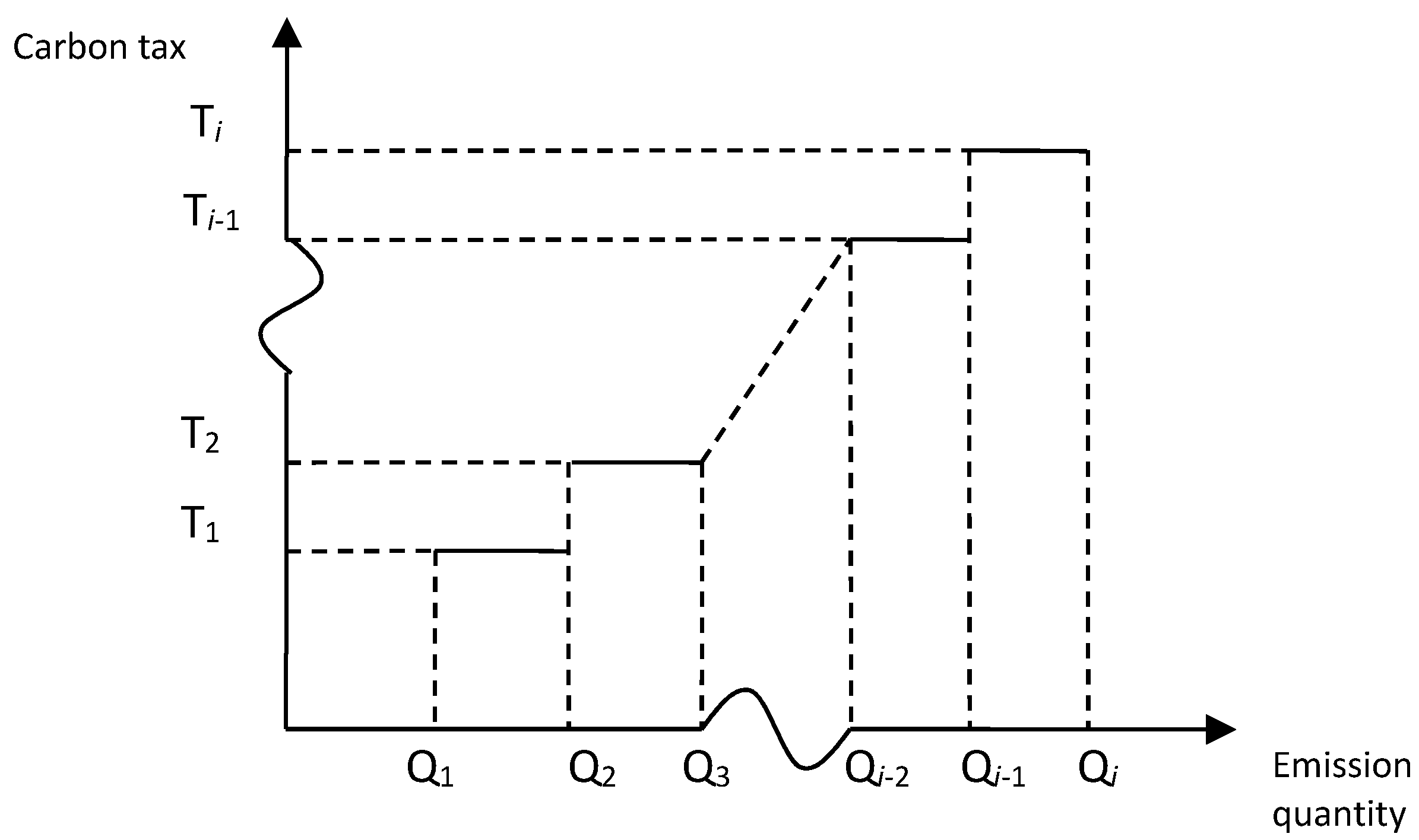
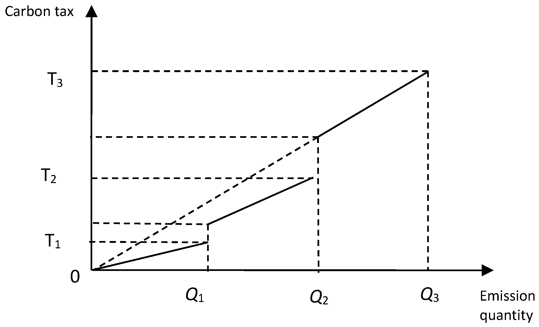
3.5. Sensitivity Test with Carbon Tax

Carbon taxes are an important taxation aimed to reduce carbon emissions and are directly related to the carbon content of fuels [6,41]; therefore, carbon taxes are levied according to the emission price per ton. The full progressive tax system, as shown in Figure 2, reports better results in carbon reductions; thus, this study intends to explore the sensitivity analysis effects of carbon tax levy methods on joint product mix decisions. In Equations (24)–(32), the carbon tax cost and the related constraints can be expressed as follows:
C a r b o n   t a x   cos   t = m 1 × D T + m 2 × E T + m 3 × F T ,
i = 1 n T A i r y i = D T + E T + F T ,
D T 0 ,
D T G 1 Q 1 ,
E T > G 2 Q 1 ,
E T G 2 Q 2 ,
F T > G 3 Q 2 ,
F T G 3 Q 3 ,
G 1 + G 2 + G 3 = 1 ,
where,
  • m r  is the carbon tax rate of the r-th carbon emission charge level;
  • Q r  is the upper limit of the r-th carbon emission charge level;
  • G r  is a zero/one variable; G r = 1 means that the carbon emission quantity is within the r-th carbon emission charge level;
  • D T , E T , F T  are the variable for the carbon emission quantity within the first, second and third carbon emission charge levels, respectively.

4. An Illustrative Case

By using the information of the pharmaceutical industry from APIs’ processing to drugs for medical use, this paper establishes TDABC, TOC and ABC joint product mix models in order to analyze the resources used and whether joint products after the split-off point are directly sold or further processed. LINGO software is used to obtain the optimal solutions of the various variables of the models, which are illustrated in the following case. Gama is a manufacturer of APIs, which produces large amounts of APIs for downstream manufacturers. Meanwhile, the company has some patented pharmaceutical technologies to add excipients into some APIs in order to process them into medication for further use and clinical purposes. In joint production Process 0, if the company inputs one pound of API raw material M0 for processing, it can produce three types of drugs after the split-off point, including D10 (one unit), D20 (one unit) and D30 (one unit). D10 and D20 are special APIs that can be further processed, and their market demands are significantly greater than D30. The required production unit labor hours, hours for each initialization hour and hours for drug inspection are the lowest, while the unit machine hours for each batch is the highest. In addition, the production process of D20 can produce the same amount of VOC1. D30 is a normal API, as compared to other APIs; its hours for each initialization and drug inspection are the highest, and the time to transfer the APIs to the production department is the longest. In addition, regarding each unit of D10, if added with excipient M11 in Process 1, it can produce one unit of D11 for each unit of D20; if added with excipient M21 in Process 2, it can produce one unit of D21. The sale prices of D11 and D21 after processing are higher than the prices of D10 and D20 at the split-off point; however, the market demand is significantly lower than D10, D20 or D30. In addition, D11 and D21 require more hours of drug inspection, and equal amounts of VOC2 and VOC3 will be produced during the production process. Therefore, the disposal costs of relevant VOCs should be borne. The company’s order processing and tableting control departments are mainly for order processing and the inspection of each batch of APIs to the tableting department. On average, each order processing takes about 20 min and requires 40 min, 40 min, 60 min, 40 min and 40 min, respectively, to transfer the produced APIs of D10, D20, D30, D11 and D21 to the tableting department; and requires about 40 min for each shipping order in the packaging and shipping departments. Moreover, it requires 6 min for the packaging of each unit of product and 10 h, 50 h and 40 h for processing each batch of VOC1, VOC2 and VOC3, respectively, and the costs are $400,000. The production process is as shown in Figure 3, and the relevant production data are as shown in Table 1.
Unlike TDABC, ABC must estimate the time percentages of various activities before the implementation of the second stage activity allocation. Therefore, in order to compute the product mix of the Gama Company under the ABC system, the following additional production information should be provided: order processing and production control departments spend about 30% in order processing and the remaining 70% in shifting the production APIs to the tableting department. The tableting department spends about 85% of its time in tableting and 15% of its time in the preparation of the tableting machine. Regarding machines and equipment, tableting requires about 90% of the time, and the initialization of the tableting machine requires about 10% of the time. Regarding the shipping department, on average, 85% of its time is for packaging, and 15% of its time is for shipping.
Regarding the above decision-making models, LINGO software is used to obtain the optimal solutions of the various variables of the model, as shown in Appendix Table A1, Table A2 and Table A3.

4.1. TDABC

Gama Company’s joint production activity information and input data are used to develop the TDABC objective function (1) and Constraints (2)–(14), as shown in Table A1; where η 0 , η i 0 , η i 1 , β i 0 , β i 1 , δ i 0 and δ i 1 are non-negative integers, τ i 0 and τ i 1 are zero and one variables. According to Table A1, under the TDABC model, the optimal product mix is the input of API M0 (30,660 pounds) for processing to produce three different types of drugs D10 (7840 units), D20 (8960 units) and D30 (5400 units) after the split-off point for direct sale to downstream drug manufacturers. Some D10 and D20 can be further processed after the split-off point to produce drugs D11 (4500 units) and D21 (3960 units). As shown in Table 2, the labor of the tableting department requires 14,368 h; the tableting machine operation requires 16,812 h; order processing requires 101 h; pharmaceutical inspection requires 900 h; shipping requires 3193 h; and VOC disposal requires 2400 h, which suggests that the maximum profit of the case company, as based on resources used, is $534,881.

4.2. TOC

By using the company’s joint production activity information and input data, the TOC objective function (15) and Constraints (2)–(14) can be expressed, as shown in Table A2; where η 0 , η i 0 , η i 1 , β i 0 , β i 1 , δ i 0 and δ i 1 are non-negative integers, τ i 0 and τ i 1 are zero and one variables. According to Table A2, under the TOC model and after the split-off point, the optimal product mix is the input of API M0 (30,880 pounds) required for processing in order to produce three different drugs, including D10 (7840 units), D20 (8400 units) and D30 (6000 units), for direct sales to downstream drug manufacturers. Some D10 and D20 can be processed for drugs D11 (4680 units) and D21 (3960 units) after the split-off point. As shown in Table 2, the tableting department’s labor requires 14,561 h; the tableting machine operation requires 16,857 h; order processing requires 104 h; pharmaceutical inspection requires 900 h; shipping requires 3217 h; and VOC disposal requires 2440 h; however, TOC makes assumptions on the basis of the resources supplied. In addition to materials, no resources will change with the production output; therefore, unused resources are recognized as costs, which suggests that the maximum profit of the company, as based on the resources supplied, is $313,870.

4.3. ABC

By using the company’s joint production activity information in Table 1 and the input data, ABC objective function (1) and Constraints (2)–(4), (8) and (9), (12)–(14) and (16)–(23) can be expressed, as in Table A3; where η 0 , η i 0 , η i 1 , β i 0 , β i 1 , δ i 0 and δ i 1 are non-negative integers, τ i 0 and τ i 1 are zero and on variables. Table A3 shows that under the ABC model, the optimal product mix is the input of API M0 (27,840 pounds) for processing in order to produce three types of drugs after the split-off point, including D10 (7840 units), D20 (8960 units) and D30 (2400 units), for direct sale to downstream drug manufacturers. Some D10 and D20 are processed to produce drugs after the split-off point, including D11 (4680 units) and D21 (3960 units). As shown in Table 2, the tableting department’s labor requires 12,928 h; the tableting machine operation requires 15,336 h; order processing requires 89 h; pharmaceutical inspection requires 900 h; shipping requires 2898 h; and VOC disposal requires 2450 h, which suggests that the maximum profit of the company, as based on the resources used, is $483,122.

4.4. Analysis

Panel A and Panel C in Table 2 show the differences of TOC, ABC and TDABC decision-making models in terms of joint product mix and profit. TOC makes assumptions on the basis of resources supplied, while ABC and TDABC make assumptions on the basis of resources used. In TDABC, the optimal joint product mix is to produce 7840 units of D10, 8960 units of D20, 5400 units of D30, 4500 units of D11 and 3960 units of D21, and the expected profit is $534,881. In TOC, the optimal joint product mix is to produce 7840 units of D10, 8400 units of D20, 6000 units of D30, 4680 units of D11 and 3960 units of D21, and the expected profit is $313,870. In ABC, the optimal joint product mix is to produce 7840 units of D10, 8960 units of D20, 2400 units of D30, 4680 units of D11 and 3960 units of D21, and the expected profit is $483,122. Therefore, profits based on resources will be the most in the TDABC system, followed by TOC and ABC. However, TDABC assumes that resources are controllable; therefore, unused production capacity can be used for other purposes or reduced. The assumptions of ABC are similar to those of TDABC; meaning unused production capacity costs can be avoided by management’s decision-making; hence, unused production capacity costs are not considered. Conversely, TOC assumes that resources are uncontrollable; therefore, unused production capacity will be regarded as cost. However, in order to compare with TOC on the basis of resources supplied, TDABC considers unused production capacity costs; thus, profit under the consideration of the basis of resources supplied is smaller or equal to the profit on the basis of the resources used. In addition, regarding the differences between ABC and TDABC in terms of profit: ABC compared to TDABC has the time and procedures of various activities at the first stage and, thus, has more constraints. As a result, the product mix will be different, and the profit will be lower than TDABC.
Panel B in Table 2 illustrates the resources used under TOC, ABC and TDABC decision-making models so that decision-makers can effectively control idle production capacity. As costs should be allocated in two stages, in the case of the ABC system, at the first stage, the company should attribute resource costs to different activity centers according to the resource drivers. At the second stage, the costs of various activities centers are attributed to various cost objectives according to cost drivers.

4.5. Sensitivity Test with Carbon Tax

This study performs sensitivity analysis to show how the optional solutions are affected by the characteristics of the carbon tax. The sensitivity test is performed with carbon tax cost (24) and the related constraints (25) to (32) by using the TDBC model shown in Table A4. The optimal product mix is the input of API M0 (30,540 pounds) for processing to produce three different types of drugs, D10 (7840 units), D20 (8960 units) and D30 (5100 units), after the split-off point for direct sales to downstream drug manufacturers. Some D10 and D20 can be further processed after the split-off point to produce drugs D11 (4680 units) and D21 (3960 units). The tableting department’s labor requires 14,368 h; the tableting machine operation requires 16,812 h; order processing requires 101 h; pharmaceutical inspection requires 900 h; shipping requires 3193 h; and VOC disposal requires 2400 h, which suggests that the maximum profit of the case company, as based on the resources used, is $420,502, and the carbon tax is $112,500.

5. Discussion

TDABC time drivers go directly from resources to cost objectives and omit the time-consuming first stage of subjective estimation, as there is no need to estimate the time percentage of various activities at the second stage. Compared to the conventional ABC, it can better reflect the reality and time differences between different activities.
In the case of profit based on resources supplied, the profit will be highest in the case of TOC, followed by TDABC and ABC. Regarding the differences in the profit between TOC and TDABC, in addition to the differences caused by product mix, the degree of control of resources by management will be one of the influencing factors. Furthermore, regarding decision-making from the perspective of resources used, management will adopt the TDABC system. However, from the viewpoint of resources supplied, management will adopt the TOC system.
The results of this study point out that ABC, as compared to TDABC, has more allocation constraints; thus, the average production capacity utility is lower than that of TDABC. In addition, under limited resources, the company should consider reducing environmental pollution in the pursuit of long-term profit. TDABC produces far fewer VOCs, as compared to TOC and ABC, suggesting that the optimal product mix model can effectively minimize waste discharge in the production process in order to reduce relevant waste disposal costs and environmental impact. To test the robustness of the above results, this study also performs sensitivity testing, where global emissions are kept, rather than the constant carbon tax rate across scenarios. In other words, this study assumes the TDABC model, as this design avoids evaluating different global emissions levels, as the emission changes are equal across the joint product mix.
In this paper, the presented decision-making models are solved using LINGO software in order to obtain the optimal solutions of the various variables of the model. In practice, a decision-maker may want to find an optimal solution under the given resource constraints. However, this optimization is conditional and depends on the preset objective structure. Since the selection of objective structures may be qualitative and must consider multiple stakeholders and criteria, this paper suggests using the LINGO model to determine the final objective structure and solution. LINGO software can solve linear, nonlinear (convex and nonconvex/global), quadratic, quadratically constrained, second order cone, semi-definite, stochastic and integer optimization models more quickly, more easily and more efficiently. Table 3 shows the limits of the various variables and constraints of the various LINGO versions. The computational performance of the LINGO model also depends on the memory available in the computer system and not only the maximum problem dimensions of LINGO capacity.

6. Conclusions

Since the 1980s, the global average temperature has risen rapidly, and unusual weather and climate phenomena frequently occur, rendering climate change an important issue. Carbon taxation is one of the most common carbon emission regulation policies that companies must incorporate in their production and pricing decisions. The aim of this paper is to apply TDABC and TOC to analyze green product mix decision-making for joint products using a mathematical programming model and the joint production data of pharmaceutical companies for processing active pharmaceutical ingredients (APIs) into drugs for medical use. This paper has three major considerations; first is to establish the joint product mix model, as based on TDABC. This decision-making model can accurately attribute used resources to the cost objective and separate unused idle production capacity for management as a reference for decision-making. Secondly, as compared to the conventional ABC model, the proposed TDABC joint product mix model is not subject to the influence of the percentages of time input in the various activities of different departments. Therefore, the optimal joint product mix has higher profit than that of the conventional ABC model, and this study performed sensitivity analysis to show how the optional solutions are affected by the characteristics of carbon tax. Third, this study proposed using MIP to solve the problem of the optimal joint product mix. In addition to converting the non-linear model into a linear model in order to obtain the global optimal solution, it can add constraints in line with reality and according to the decisions of management.
The empirical results show that profit based on resources will be the most in the system of TDABC, followed by TOC and ABC; while for decision-making according to the perspective of the resources used basis, management will prefer the TDABC system. However, from the viewpoint of the resources supplied basis, management will prefer the TOC system. Finally, as compared to TDABC, ABC has more allocation constraints; thus, the average production capacity utility is lower than that of TDABC.
By using the example of a pharmaceutical company, this study illustrates the feasibility of TDABC in a joint product mix, which is expected to integrate the conceptual structure with the various modules of the enterprise resource planning (ERP) system for analysis and application in companies of other industries, in order to help managers effectively improve processes, reduce costs, analyze value, modify strategy and make other decisions. Compared to traditional costing, more comprehensive tools and concepts are available to analyze material, carbon emissions and energy flows within production systems, as well as their financial and ecological consequences. In addition, limited by the production activity information, as provided by the case company, this study cannot learn the production strategy in the case of insufficient production capacity. Future studies can further consider improving long-term production capacity insufficiency through production strategies, such as outsourcing and increasing labor or equipment in response to market demand to satisfy customer orders and maximize company profits. As a new management and accounting tool, relevant literature and discussions regarding TDABC are insufficient; thus, future studies can apply other management and strategy dimensions, such as the agent-based simulation model and corporate carbon footprint management.
This paper was based on some specific assumptions; for example, this paper assumed that potential competitors’ prices are not sensitive to the temporary price changes of a company’s product in the short term. In future studies, researchers can relax the assumptions to explore more complicated and realistic situations.

Acknowledgments

The authors are extremely grateful to the Sustainability journal editorial team and reviewers who provided valuable comments for improving the quality of this article. The authors also would like to thank the Ministry of Science and Technology of Taiwan for partial financial support of this research under Grant No. MOST104-2410-H-008-045.

Author Contributions

Wen-Hsien Tsai and Chu-Lun Hsieh provided the research idea, the research purpose and designed the research. Jui-Chu Chang provided the research and the research method, and revised this paper. Chu-Lun Hsieh, Tsen-Shu Tsaur and Chung-Wei Wang collected and analyzed the data and wrote the paper. Wen-Hsien Tsai provided the research method, supervised, corrected and revised this paper. All authors have read and approved the final manuscript.

Appendix A

Table A1. Optimal joint product mix decision analysis of the TDABC model.
M a x    π = 145 × η 10 + 140 × η 20 + 125 × η 30 + 160 × η 11 + 180 × η 21 70 × η 0 20 × η 11 25 × η 21 38.5 × ( 0.3 × η 10 + 0.4 × η 20 + 0.5 × η 30 + 0.6 × η 11 + 0.7 × η 21 ) 25.5 × ( 0.7 × η 10 + 0.6 × η 20 + 0.5 × η 30 + 0.4 × η 11 + 0.3 × η 21 ) 38.5 × ( 2 × β 10 + 3 × β 20 + 5 × β 30 + 2 × β 11 + 2 × β 21 ) 25.5 × ( 2 × β 10 + 3 × β 20 + 5 × β 30 + 2 × β 11 + 2 × β 21 ) 20 × 40 × ( β 10 + β 20 + β 30 + β 11 + β 21 ) ÷ 60    40 × ( 40 β 10 + 40 β 20 + 60 β 30 + 40 β 11 + 40 β 21 ) ÷ 60    30 × ( 40 × δ 10 + 40 × δ 20 + 40 × δ 30 + 40 × δ 11 + 40 × δ 21 ) ÷ 60 30 × ( 6 × η 10 + 6 × η 20 + 6 × η 30 + 6 × η 11 + 6 × η 21 ) ÷ 60 70.25 × ( 100 × τ 10 + 100 × τ 20 + 150 × τ 30 + 300 × τ 11 + 250 × τ 21 ) 35 × ( 10 β 20 + 50 β 11 + 45 β 21 ) 400 , 000
Subject to Direct Material
η 0 = η 10 + η 20 + η 30 + η 11 + η 21 η 10 ÷ β 10 = 560            η 20 ÷ β 20 = 560           η 30 ÷ β 30 = 300 η 11 ÷ β 11 = 180             η 21 ÷ β 21 = 180
Subject to Tableting Labor
0.3 × η 10 + 0.4 × η 20 + 0.5 × η 30 + 0.6 × η 11 + 0.7 × η 21 + 2 × β 10 + 3 × β 20 + 5 × β 30 + 2 × β 11 + 2 × β 21 18 , 640
Subject to Tableting Machinery
0.7 × η 10 + 0.6 × η 20 + 0.5 × η 30 + 0.4 × η 11 + 0.3 × q 21 + 2 × β 10 + 3 × β 20 + 5 × β 30 + 2 × β 11 + 2 × β 21 16 , 880
Subject to Inspection
100 × τ 10 + 100 × τ 20 + 150 × τ 30 + 300 × τ 11 + 250 × τ 21 1000 η 10 8000 × τ 10       η 20 9000 × τ 20      η 30 6000 × τ 30     η 11 4800 × τ 11       η 21 4400 × τ 21
Subject to VOCs Disposal
10 × β 20 + 50 × β 11 + 45 × β 21 3000
Subject to Ordering
20 × β 10 + 20 × β 20 + 20 × β 30 + 20 × β 11 + 20 × β 21 + 40 × β 10 + 40 × β 20 + 60 × β 30 + 40 × β 11 + 40 × β 21 250 × 60
Subject to Shipping
40 δ 10 + 40 δ 20 + 40 δ 30 + 40 δ 11 + 40 δ 21 + 6 η 10 + 6 η 20 + 6 η 30 + 6 η 11 + 6 η 21 4100 × 60 η 10 = 280 × δ 10       η 20 = 280 × δ 20       η 30 = 150 × δ 30 η 11 = 90 × δ 11            η 21 = 90 × δ 21
Optimal Joint Product Mix Solution for the TDABC Model
η 0 = 30 , 660       η 10 = 7840       η 20 = 8960      η 30 = 5400      η 11 = 4500       η 21 = 3960      β 10 = 14      β 20 = 16       β 30 = 18      β 11 = 25          β 21 = 22       δ 10 = 28       δ 20 = 32      δ 30 = 36 δ 11 = 50         δ 21 = 44        τ 10 = 1      τ 20 = 1       τ 30 = 1      τ 11 = 1          τ 21 = 1
Table A2. Optimal joint product mix decision analysis of the TOC model.
M a x    π = 145 × η 10 + 140 × η 20 + 125 × η 30 + 160 × η 11 + 180 × η 21 70 × η 0 20 × η 11 25 × η 21 717 , 640 430 , 440 10 , 000 123 , 000 70 , 250 10 , 500 400 , 000             
Subject to Direct Material
η 0 = η 10 + η 20 + η 30 + η 11 + η 21 η 10 ÷ β 10 = 560            η 20 ÷ β 20 = 560           η 30 ÷ β 30 = 300 η 11 ÷ β 11 = 180             η 21 ÷ β 21 = 180
Subject to Tableting Labor
0.3 × η 10 + 0.4 × η 20 + 0.5 × η 30 + 0.6 × η 11 + 0.7 × η 21 + 2 × β 10 + 3 × β 20 + 5 × β 30 + 2 × β 11 + 2 × β 21 18 , 640
Subject to Tableting Machinery
0.7 × η 10 + 0.6 × η 20 + 0.5 × η 30 + 0.4 × η 11 + 0.3 × q 21 + 2 × β 10 + 3 × β 20 + 5 × β 30 + 2 × β 11 + 2 × β 21 16 , 880
Subject to Inspection
100 × τ 10 + 100 × τ 20 + 150 × τ 30 + 300 × τ 11 + 250 × τ 21 1000 η 10 8000 × τ 10       η 20 9000 × τ 20      η 30 6000 × τ 30     η 11 4800 × τ 11       η 21 4400 × τ 21
Subject to VOCs Disposal
10 × β 20 + 50 × β 11 + 45 × β 21 3000
Subject to Ordering
20 × β 10 + 20 × β 20 + 20 × β 30 + 20 × β 11 + 20 × β 21 + 40 × β 10 + 40 × β 20 + 60 × β 30 + 40 × β 11 + 40 × β 21 250 × 60
Subject to Shipping
40 δ 10 + 40 δ 20 + 40 δ 30 + 40 δ 11 + 40 δ 21 + 6 η 10 + 6 η 20 + 6 η 30 + 6 η 11 + 6 η 21 4100 × 60 η 10 = 280 × δ 10       η 20 = 280 × δ 20       η 30 = 150 × δ 30 η 11 = 90 × δ 11            η 21 = 90 × δ 21
Optimal Joint Product Mix Solution for the TDABC Model
η 0 = 30 , 880       η 10 = 7840       η 20 = 8400      η 30 = 6000      η 11 = 4680       η 21 = 3960      β 10 = 14      β 20 = 15       β 30 = 20     β 11 = 26          β 21 = 22       δ 10 = 28       δ 20 = 30      δ 30 = 40 δ 11 = 52         δ 21 = 44        τ 10 = 1      τ 20 = 1       τ 30 = 1      τ 11 = 1          τ 21 = 1
Table A3. Optimal joint product mix decision analysis of the ABC model.
M a x    π = 145 × η 10 + 140 × η 20 + 125 × η 30 + 160 × η 11 + 180 × η 21 70 × η 0 20 × η 11 25 × η 21 38.5 × ( 0.3 × η 10 + 0.4 × η 20 + 0.5 × η 30 + 0.6 × η 11 + 0.7 × η 21 ) 25.5 × ( 0.7 × η 10 + 0.6 × η 20 + 0.5 × η 30 + 0.4 × η 11 + 0.3 × η 21 ) 38.5 × ( 2 × β 10 + 3 × β 20 + 5 × β 30 + 2 × β 11 + 2 × β 21 ) 25.5 × ( 2 × β 10 + 3 × β 20 + 5 × β 30 + 2 × β 11 + 2 × β 21 ) 20 × 40 × ( β 10 + β 20 + β 30 + β 11 + β 21 ) ÷ 60    40 × ( 40 β 10 + 40 β 20 + 60 β 30 + 40 β 11 + 40 β 21 ) ÷ 60    30 × ( 40 × δ 10 + 40 × δ 20 + 40 × δ 30 + 40 × δ 11 + 40 × δ 21 ) ÷ 60 30 × ( 6 × η 10 + 6 × η 20 + 6 × η 30 + 6 × η 11 + 6 × η 21 ) ÷ 60 70.25 × ( 100 × τ 10 + 100 × τ 20 + 150 × τ 30 + 300 × τ 11 + 250 × τ 21 ) 35 × ( 10 β 20 + 50 β 11 + 45 β 21 ) 400 , 000
Subject to Direct Material
η 0 = η 10 + η 20 + η 30 + η 11 + η 21 η 10 ÷ β 10 = 560            η 20 ÷ β 20 = 560           η 30 ÷ β 30 = 300 η 11 ÷ β 11 = 180             η 21 ÷ β 21 = 180
Subject to Ordering
20 × β 10 + 20 × β 20 + 20 × β 30 + 20 × β 11 + 20 × β 21 15 , 000 × 0.3 40 × β 10 + 40 × β 20 + 60 × β 30 + 40 × β 11 + 40 × β 21 15 , 000 × 0.7
Subject to Tableting Labor
0.3 × η 10 + 0.4 × η 20 + 0.5 × η 30 + 0.6 × η 11 + 0.7 × η 21 + 2 × β 10 + 3 × β 20 + 5 × β 30 + 2 × β 11 + 2 × β 21 18 , 640 × 0.85 2 × β 10 + 3 × β 20 + 5 × β 30 + 2 × β 11 + 2 × β 21 18 , 640 × 0.15
Subject to Tableting Machinery
0.7 × η 10 + 0.6 × η 20 + 0.5 × η 30 + 0.4 × η 11 + 0.3 × q 21 + 2 × β 10 + 3 × β 20 + 5 × β 30 + 2 × β 11 + 2 × β 21 16 , 880 × 0.9 2 × β 10 + 3 × β 20 + 5 × β 30 + 2 × β 11 + 2 × β 21 16 , 880 × 0.1
Subject to Inspection
100 × τ 10 + 100 × τ 20 + 150 × τ 30 + 300 × τ 11 + 250 × τ 21 1000 η 10 8000 × τ 10       η 20 9000 × τ 20      η 30 6000 × τ 30     η 11 4800 × τ 11       η 21 4400 × τ 21
Subject to VOCs Disposal
10 × β 20 + 50 × β 11 + 45 × β 21 3000
Subject to Shipping
40 δ 10 + 40 δ 20 + 40 δ 30 + 40 δ 11 + 40 δ 21 + 6 η 10 + 6 η 20 + 6 η 30 + 6 η 11 + 6 η 21 4100 × 60 × 0.15 6 × η 10 ÷ 60 + 6 × η 20 ÷ 60 + 6 × η 30 ÷ 60 + 6 × η 11 ÷ 60 + 6 × η 21 ÷ 60 4100 × 0.85 η 10 = 280 × δ 10       η 20 = 280 × δ 20       η 30 = 150 × δ 30 η 11 = 90 × δ 11            η 21 = 90 × δ 21
Optimal Joint Product Mix Solution for the TDABC Model
η 0 = 27 , 840       η 10 = 7840       η 20 = 8960      η 30 = 2400      η 11 = 4680       η 21 = 3960      β 10 = 14      β 20 = 16       β 30 = 8      β 11 = 26          β 21 = 22       δ 10 = 28       δ 20 = 32      δ 30 = 16 δ 11 = 52         δ 21 = 44        τ 10 = 1      τ 20 = 1       τ 30 = 1      τ 11 = 1          τ 21 = 1
Table A4. Sensitivity analysis of TDABC model with the carbon tax.
M a x    π = 145 × η 10 + 140 × η 20 + 125 × η 30 + 160 × η 11 + 180 × η 21 70 × η 0 20 × η 11 25 × η 21 38.5 × ( 0.3 × η 10 + 0.4 × η 20 + 0.5 × η 30 + 0.6 × η 11 + 0.7 × η 21 ) 25.5 × ( 0.7 × η 10 + 0.6 × η 20 + 0.5 × η 30 + 0.4 × η 11 + 0.3 × η 21 ) 38.5 × ( 2 × β 10 + 3 × β 20 + 5 × β 30 + 2 × β 11 + 2 × β 21 ) 25.5 × ( 2 × β 10 + 3 × β 20 + 5 × β 30 + 2 × β 11 + 2 × β 21 ) 20 × 40 × ( β 10 + β 20 + β 30 + β 11 + β 21 ) ÷ 60    40 × ( 40 β 10 + 40 β 20 + 60 β 30 + 40 β 11 + 40 β 21 ) ÷ 60    30 × ( 40 × δ 10 + 40 × δ 20 + 40 × δ 30 + 40 × δ 11 + 40 × δ 21 ) ÷ 60 30 × ( 6 × η 10 + 6 × η 20 + 6 × η 30 + 6 × η 11 + 6 × η 21 ) ÷ 60 70.25 × ( 100 × τ 10 + 100 × τ 20 + 150 × τ 30 + 300 × τ 11 + 250 × τ 21 ) 35 × ( 10 β 20 + 50 β 11 + 45 β 21 ) ( 3 × D T + 4 × E T + 5 × F T ) 400 , 000
Subject to Direct Material
η 0 = η 10 + η 20 + η 30 + η 11 + η 21 η 10 ÷ β 10 = 560            η 20 ÷ β 20 = 560           η 30 ÷ β 30 = 300 η 11 ÷ β 11 = 180             η 21 ÷ β 21 = 180
Subject to Tableting Labor
0.3 × η 10 + 0.4 × η 20 + 0.5 × η 30 + 0.6 × η 11 + 0.7 × η 21 + 2 × β 10 + 3 × β 20 + 5 × β 30 + 2 × β 11 + 2 × β 21 18 , 640
Subject to Tableting Machinery
0.7 × η 10 + 0.6 × η 20 + 0.5 × η 30 + 0.4 × η 11 + 0.3 × q 21 + 2 × β 10 + 3 × β 20 + 5 × β 30 + 2 × β 11 + 2 × β 21 16 , 880
Subject to Inspection
100 × τ 10 + 100 × τ 20 + 150 × τ 30 + 300 × τ 11 + 250 × τ 21 1000 η 10 8000 × τ 10       η 20 9000 × τ 20      η 30 6000 × τ 30     η 11 4800 × τ 11       η 21 4400 × τ 21
Subject to Carbon Tax
3 × η 30 + 2 × η 11 + 2 × η 21 D T + E T + F T D T 0         D T G 1 × 12 , 000       E T > G 2 × 12 , 000       E T G 2 × 15 , 000 F T > G 3 × 15 , 000       F T G 3 × 25 , 000 G 1 + G 2 + G 3 = 1         
Subject to Ordering
20 × β 10 + 20 × β 20 + 20 × β 30 + 20 × β 11 + 20 × β 21 + 40 × β 10 + 40 × β 20 + 60 × β 30 + 40 × β 11 + 40 × β 21 250 × 60
Subject to Shipping
40 δ 10 + 40 δ 20 + 40 δ 30 + 40 δ 11 + 40 δ 21 + 6 η 10 + 6 η 20 + 6 η 30 + 6 η 11 + 6 η 21 4100 × 60 η 10 = 280 × δ 10       η 20 = 280 × δ 20       η 30 = 150 × δ 30 η 11 = 90 × δ 11            η 21 = 90 × δ 21
Subject to VOCs Disposal
10 × β 20 + 50 × β 11 + 45 × β 21 3000
Sensitivity Analysis of TDABC Model with the Carbon Tax
η 0 = 30 , 540       η 10 = 7840       η 20 = 8960      η 30 = 5100      η 11 = 4680       η 21 = 3960      β 10 = 14      β 20 = 16       β 30 = 17      β 11 = 26          β 21 = 22       δ 10 = 28       δ 20 = 32      δ 30 = 34 δ 11 = 52         δ 21 = 44        τ 10 = 1      τ 20 = 1       τ 30 = 1      τ 11 = 1          τ 21 = 1            C T = 10 , 000          D T = 0           E T = 0        F T = 22 , 500         G 1 = 1          G 2 = 0          G 3 = 0         G 4 = 0   

References

  1. Tsai, W.H.; Lai, C.W.; Tseng, L.J.; Chou, W.C. Embedding management discretionary power into an ABC model for joint product mix decisions. Int. J. Prod. Econom. 2008, 115, 210–220. [Google Scholar]
  2. Tsai, W.H. Activity-based costing model for joint products. Comput. Ind. Eng. 1996, 31, 725–729. [Google Scholar]
  3. Hartley, R.V. Decision making when joint products are involved. Account. Rev. 1971, 46, 746–755. [Google Scholar]
  4. Kee, R.; Schmidt, C. A comparative analysis of utilizing activity-based costing and the theory of 3 constraints for making product-mix decisions. Int. J. Prod. Econom. 2000, 63, 1–17. [Google Scholar] [CrossRef]
  5. Onwubolu, G.C.; Muting, M. Optimizing the multiple constrained resources product mix problem using genetic algorithms. Int. J. Prod. Res. 2001, 39, 1897–1910. [Google Scholar] [CrossRef]
  6. Tsai, W.-H.; Lee, K.-C.; Liu, J.-Y.; Lin, H.-L.; Chou, Y.-W.; Lin, S.-J. A mixed activity-based costing decision model for green airline fleet planning under the constraints of the European Union Emissions Trading Scheme. Energy 2012, 39, 218–226. [Google Scholar] [CrossRef]
  7. Kirche, E.; Srivastava, R. An ABC-based cost model with inventory and order level costs: A comparison with TOC. Int. J. Prod. Res. 2005, 43, 1685–1710. [Google Scholar] [CrossRef]
  8. Gong, Z.; Hu, S. An economic evaluation model of product mix flexibility. Omega 2008, 36, 852–864. [Google Scholar]
  9. Turney, P.B. Common Cents: The ABC Performance Breakthrough: How to Succeed with Activity-Based Costing; Cost Technology: Hillsboro, OR, USA, 1991. [Google Scholar]
  10. Plenert, G. Optimizing theory of constraints when multiple constrained resources exist. Eur. J. Oper. Res. 1993, 70, 126–133. [Google Scholar] [CrossRef]
  11. Souren, R.; Ahn, H.; Schmitz, C. Optimal product mix decisions based on the theory of constraints. Exposing rarely emphasized premises of throughput accounting. Int. J. Prod. Res. 2005, 43, 361–374. [Google Scholar] [CrossRef]
  12. Fredendall, L.D.; Lea, B.R. Improving the product mix heuristic in the theory of constraints. Int. J. Prod. Res. 1997, 35, 1535–1544. [Google Scholar] [CrossRef]
  13. Pernot, E.; Roodhooft, F.; Van den Abbeele, A. Time-driven activity-based costing for inter-library services: A case study in a university. J. Acad. Librariansh. 2007, 33, 551–560. [Google Scholar] [CrossRef]
  14. Szychta, A. Time-Driven Activity-Based Costing in Service Industries. Soc. Sci. 2010, 67, 49–60. [Google Scholar]
  15. Stouthuysen, K.; Swiggers, M.; Reheul, A.-M.; Roodhooft, F. Time-driven activity-based costing for a library acquisition process: A case study in a Belgian University. Lib. Collect. Acquis. Tech. Serv. 2010, 34, 83–91. [Google Scholar] [CrossRef]
  16. Öker, F.; Adigüzel, H. Time-driven activity-based costing: An implementation in a manufacturing company. J. Corp. Account. Financ. 2010, 22, 75–92. [Google Scholar] [CrossRef]
  17. Tsai, W.-H.; Shen, Y.-S.; Lee, P.-L.; Chen, H.-C.; Kuo, L.; Huang, C.-C. Integrating information about the cost of carbon through activity-based costing. J. Clean. Prod. 2012, 36, 102–111. [Google Scholar] [CrossRef]
  18. Friedman, M. The Social Responsibility of Business Is to Increase Its Profits. The New York Times Magazine, 13 September 1970. [Google Scholar]
  19. Carroll, A.B. The pyramid of corporate social responsibility: Toward the moral management of organizational stakeholders. Bus. Horiz. 1991, 34, 39–48. [Google Scholar] [CrossRef]
  20. Tsai, W.-H.; Chen, H.-C.; Leu, J.-D.; Chang, Y.-C.; Lin, T.W. A product-mix decision model using green manufacturing technologies under activity-based costing. J. Clean. Prod. 2013, 57, 178–187. [Google Scholar] [CrossRef]
  21. Demeere, N.; Stouthuysen, K.; Roodhooft, F. Time-driven activity-based costing in an outpatient clinic environment: Development, relevance, and managerial impact. Health Policy 2009, 92, 296–304. [Google Scholar] [CrossRef] [PubMed]
  22. Tsai, W.-H.; Yang, C.-H.; Chang, J.-C.; Lee, H.-L. An Activity-Based Costing Decision Model for Life Cycle Assessment in Green Building Projects. Eur. J. Oper. Res. 2014, 238, 607–619. [Google Scholar] [CrossRef]
  23. Cooper, R.; Kaplan, R.S. Measure costs right: Make the right decisions. Harv. Bus. Rev. 1988, 66, 96–103. [Google Scholar]
  24. Tsai, W.-H.; Hung, S.-J. A Fuzzy Goal Programming Approach for Green Supply Chain Optimisation under Activity-Based Costing and Performance Evaluation with a Value-chain Structure. Int. J. Prod. Res. 2009, 47, 4991–5017. [Google Scholar] [CrossRef]
  25. Tsai, W.-H.; Hsu, J.-L.; Chen, C.-H.; Chou, Y.-W.; Lin, S.-J.; Lin, W.-R. Application of ABC in hot spring country inn. Int. J. Manag. Enterp. Dev. 2010, 8, 152–174. [Google Scholar] [CrossRef]
  26. Kaplan, R.S.; Cooper, R. Cost & Effect: Using Integrated Cost Systems to Drive Profitability and Performance; Harvard Business School Press: Boston, MA, USA, 1998. [Google Scholar]
  27. Kaplan, R.S.; Anderson, S.R. Time-driven activity-based costing. Harv. Bus. Rev. 2004, 82, 131–140. [Google Scholar] [CrossRef] [PubMed]
  28. Kaplan, R.; Anderson, S.R. Time-Driven Activity-Based Costing: A Simpler and More Powerful Path to Higher Profits; Harvard Business School Press: Boston, MA, USA, 2013. [Google Scholar]
  29. Stouthuysen, K.; Schierhout, K.; Roodhooft, F.; Reusen, E. Time-driven activity-based costing for public services. Public Money Manag. 2014, 34, 289–296. [Google Scholar] [CrossRef]
  30. Öker, F.; Özyapici, H. A New Costing Model in Hospital Management: Time-Driven Activity-Based Costing System. Health Care Manag. 2013, 32, 23–36. [Google Scholar] [CrossRef] [PubMed]
  31. Varila, M.; Seppänen, M.; Suomala, P. Detailed cost modelling: A case study in warehouse logistics. Int. J. Phys. Distrib. Logist. Manag. 2007, 37, 184–200. [Google Scholar] [CrossRef]
  32. Kaplan, R.S.; Norton, D.P. Mastering the management system. Harv. Bus. Rev. 2008, 86, 62–77. [Google Scholar] [PubMed]
  33. Huang, S.-Y.; Chen, H.-J.; Chiu, A.-A.; Chen, C.-P. The application of the theory of constraints and activity-based costing to business excellence: The case of automotive electronics manufacture firms. Total Q. Manag. Bus. Excell. 2014, 25, 532–545. [Google Scholar] [CrossRef]
  34. Tsai, W.-H.; Chou, W.-C. Selecting Management Systems for Sustainable Development in SMEs: A Novel Hybrid Model Based on DEMATEL, ANP, and ZOGP. Expert Syst. Appl. 2009, 36, 1444–1458. [Google Scholar] [CrossRef]
  35. Goldratt, E.M.C.J. The Goal: A Process of Ongoing Improvement; Creda Press: Cape Town, South Africa, 1984. [Google Scholar]
  36. Aryanezhad, M.; Komijan, A. An improved algorithm for optimizing product mix under the theory of constraints. Int. J. Prod. Res. 2004, 42, 4221–4233. [Google Scholar] [CrossRef]
  37. Kee, R. The sufficiency of product and variable costs for production-related decisions when economies of scope are present. Int. J. Prod. Econom. 2008, 114, 682–696. [Google Scholar] [CrossRef]
  38. Tsai, W.-H.; Lai, C.-W.; Chang, J. An algorithm for optimizing joint products decisions, as based on the Theory of Constraints. Int. J. Prod. Res. 2007, 45, 3421–3437. [Google Scholar] [CrossRef]
  39. Tsai, W.-H.; Lai, C.-W. Outsourcing or capacity expansions: Application of activity-based costing model on joint products decisions. Comput. Oper. Res. 2007, 34, 3666–3681. [Google Scholar] [CrossRef]
  40. Tehrani Nejad Moghaddam, A.; Michelot, C. A contribution to the linear programming approach to joint cost allocation: Methodology and application. Eur. J. Oper. Res. 2009, 197, 999–1011. [Google Scholar] [CrossRef]
  41. Tsai, W.-H.; Lin, S.-J.; Liu, J.-Y.; Lin, W.-R.; Lee, K.-C. Incorporating Life Cycle Assessments into Building Project Decision Making: An Energy Consumption and CO2 Emission Perspective. Energy 2011, 36, 3022–3029. [Google Scholar] [CrossRef]
  42. Maximum Problem Dimensions. Available online: http://www.lindo.com/doc/online_help/lingo15_0/maximum_problem_dimensions.htm (accessed on 26 November 2016).
Figure 1. The fixed tax rate schedule.
Sustainability 08 01232 g001
Figure 2. The full progressive tax rate.
Sustainability 08 01232 g002
Figure 3. Pharmaceutical production flow chart.
Sustainability 08 01232 g003
Table 1. Example data.
Panel A: Production InformationProcess 0Process 1Process 2
Product
D10
Product
D20
Product
D30
Product
D11
Product
D21
Maximum demandRi0Ri180009000600048004000
Selling priceXi0Xi1$145$144$135$155$155
Production Coefficienteifi11111
Material of APIsMA0MAi1 $70 $20$25
Labor hourstli0tli10.30.40.50.60.7
Machine hourstmi0tmi10.70.60.50.40.3
Setup hourstbi0tbi123522
Inspection hourstτi0tτi1100100150300250
VOC disposal hours (per batch) 10 5045
Quantity of batchbi0bi1560560300180180
Quantity of shipmentsi0si12802801509090
Carbon Tax Constraint
Carbon tax rate: m1 = $3/unit; m2 = $4/unit; m3 = $5/unit
The upper limit of three carbon emission charge level: Q1 = 12,000; Q2 = 15,000; Q3 = 25,000 322
Marketing, plant guard and management $400,000
Panel B: Resources ConsumedTableting LaborTableting MachineryOrderingShippingInspectionVOC’s Disposal
Resources$717,640$430,440$10,000$123,000$70,250$105,000
Available capacity (hours) σ l = 18,640 σ m = 16,880 σ o = 250 σ δ = 4100 σ τ = 1000 σ v = 3000
Per hour/ratekl = $38.5/hkm = $25.5/hko = $40/hkδ = $30/hkτ = $70.25/hkv = $35/h
Table 2. Company Gama’s comparative analysis of the three decision models.
Panel A: Quantity of Products SoldTDABCTOCABC
Product D10784078407840
Product D20896084008960
Product D30540060002400
Product D11450046804680
Product D21396039603960
Panel B: Resources ConsumedTDABCTOCABC
Capacity (h)ConsumedConsumedConsumed
(h)(%)(h)(%)(h)(%)
Tableting labor18,64014,36877.0814,56178.1212,92869.36
Tableting machinery16,88016,81299.6016,85799.8615,33690.85
Ordering25010140.4010441.608935.60
Inspection100090090.0090090.0090090.00
Shipping 4100319377.88321778.46289870.68
VOC’s disposal3000240080.00244081.33245081.67
Panel C: ProfitTDABCTOCABC
Revenue$4,499,000$4,524,400$4,152,800
Material costs$2,335,200$2,354,200$2,141,400
Tableting labor$553,168$560,599$497,728
Tableting machinery$428,706$429,854$391,068
Ordering cost$4040$4147$3547
Inspection cost$63,225$63,225$63,225
Shipping cost$95,780$96,520$86,960
VOC’s disposal cost$84,000$85,400$85,750
Marketing, Plant guard & management$400,000$400,000$400,000
Income based on resources used in production$534,881$530,455$483,122
Unused capacity cost$227,411$216,585$328,052
Income based on resources supplied to production$307,470$313,870$155,070
Table 3. The limits for the various LINGO versions.
VersionTotal VariablesInteger VariablesNonlinear VariablesConstraints
Super Lingo20002002001000
Hyper Lingo80008008004000
Industrial Lingo32,0003200320016,000
Extended LingoUnlimitedUnlimitedUnlimitedUnlimited
Source: [42].

