Analysis of the Effectiveness of Urban Land-Use-Change Models Based on the Measurement of Spatio-Temporal, Dynamic Urban Growth: A Cellular Automata Case Study

Abstract

Developing countries have been undergoing dramatic urban growth over the past three decades. It is essential to understand and simulate the urban growth process for smart urban planning and sustainable development purposes. Cellular automata (CA) modeling is an efficient approach to simulating urban land use/cover change; however, the traditional CA method has limitations in simulating the various urban growth patterns and processes. This study aims to analyze the influences of different urban growth characteristics on the effectiveness of CA modeling by conducting a case study over the area in the Pearl River Delta of Southern China. We used the growth rate, landscape expansion index, and spatial dependency to quantify the urban growth characteristics. The effectiveness of CA modeling was measured through a comparison of the simulation results with the reference data. The simulation results and validation analyses reveal that the traditional CA is not applicable for the following three situations: (1) the urban growth pattern characterized by less growth area or a higher ratio of outlying expansion; (2) the urban region that includes several subregions with disparate growth characteristics; and (3) the existence of temporal differences in growth characteristics over a long period.

1. Introduction

Urban growth, a complex spatial process, is an important social and economic phenomenon in developing countries. Dramatic changes in the urban landscape (built-up areas) have occurred in the fast-developing regions over the past three decades. Critics of rapid growth are concerned with the alleged negative impacts, such as increased energy consumption, environmental pollution, residential crowding, traffic congestion, and irreversible damage to ecosystems [1,2,3,4,5,6]. Therefore, analyzing and predicting the spatio-temporal dynamics of urban growth is significant for smart urban planning, resource management, and sustainable development in rapidly changing environments [6,7].

Dynamic spatial modeling is essential for the analysis and especially for the simulation and prediction of the urban growth process [6,8]. Rapid progress in computer science, remote sensing, and geographic information systems technology have facilitated the emerging of various efficient dynamic spatial modeling approaches, such as cellular automata (CA), CLUE-S models [7], and multi-agent models [9]. Using these models, urban planners and policy-makers can analyze the different scenarios of urban growth and further evaluate their impacts to support policy-making on urban planning and sustainable development [10]. Among those spatial modeling approaches, the CA method is the most widely used for modeling urban dynamics. It is a bottom-up simulation approach that relies on the transition rules to model the behavior of complex systems [11]. Effective urban CA models have been developed based on statistical or data-mining techniques [12,13,14,15,16]. These techniques require observational data or historical data for the study area to calibrate the CA transition rules.

Despite the fact that the CA models have provided insights into the urban expansion dynamics, some empirical studies point out that the effectiveness of CA varies when it is applied to different cities [17]. Using fixed transition rules can result in large simulation errors because of the spatio-temporal heterogeneity at a large spatial scale or over a long period [18,19]. Previous studies have noted the relationship between urban growth characteristics and effectiveness (or applicability) of CA. However, the majority of related studies focus on qualitative analyses, whereas others lack quantitative studies.

In general, CA is implemented by using newly collected samples to rebuild the models. However, collecting the samples of land use/cover change from remote sensing imagery is extremely time-consuming and inefficient for most cases (e.g., for inexperienced users or in relatively inaccessible locations) [20]. Li and Liu have proposed the domain adaptation of CA by coupling logistic CA with a knowledge transfer technique [17]. They used the old samples that were collected from different cities to calibrate the CA transition rules and then apply these improved rules to a new urban growth simulation. This study indicates that the CA models, without using knowledge transfer, can be used to simulate the urban growth dynamics on the condition that the historical trend of urban growth continues. The reusability (or domain adaptation) of CA in different urban growth simulation models is appealing for a number of reasons: (1) inexperienced users do not need to build a brand new CA model; (2) collecting a new set of samples is not necessary; and (3) past experiences or old data are useful for capturing long-term trends. However, less attention is paid to the reusability of CA for urban growth simulations in different cities.

This paper aims to study the applicability of CA modeling for different cities that are characterized by disparate spatio-temporal characteristics of urban growth. We attempt to measure the urban growth spatio-temporal characteristics based on urban growth area and rate, spatial distance relationships, and landscape expansion index (LEI). The measurements are compared with the logistic CA to determine the accuracy of modeling urban growth processes in different scenarios. Urban growth over two time periods, 1990–2000 and 2000–2009, in the Pearl River Delta of Southern China is analyzed and modeled.

2. Materials and Methods

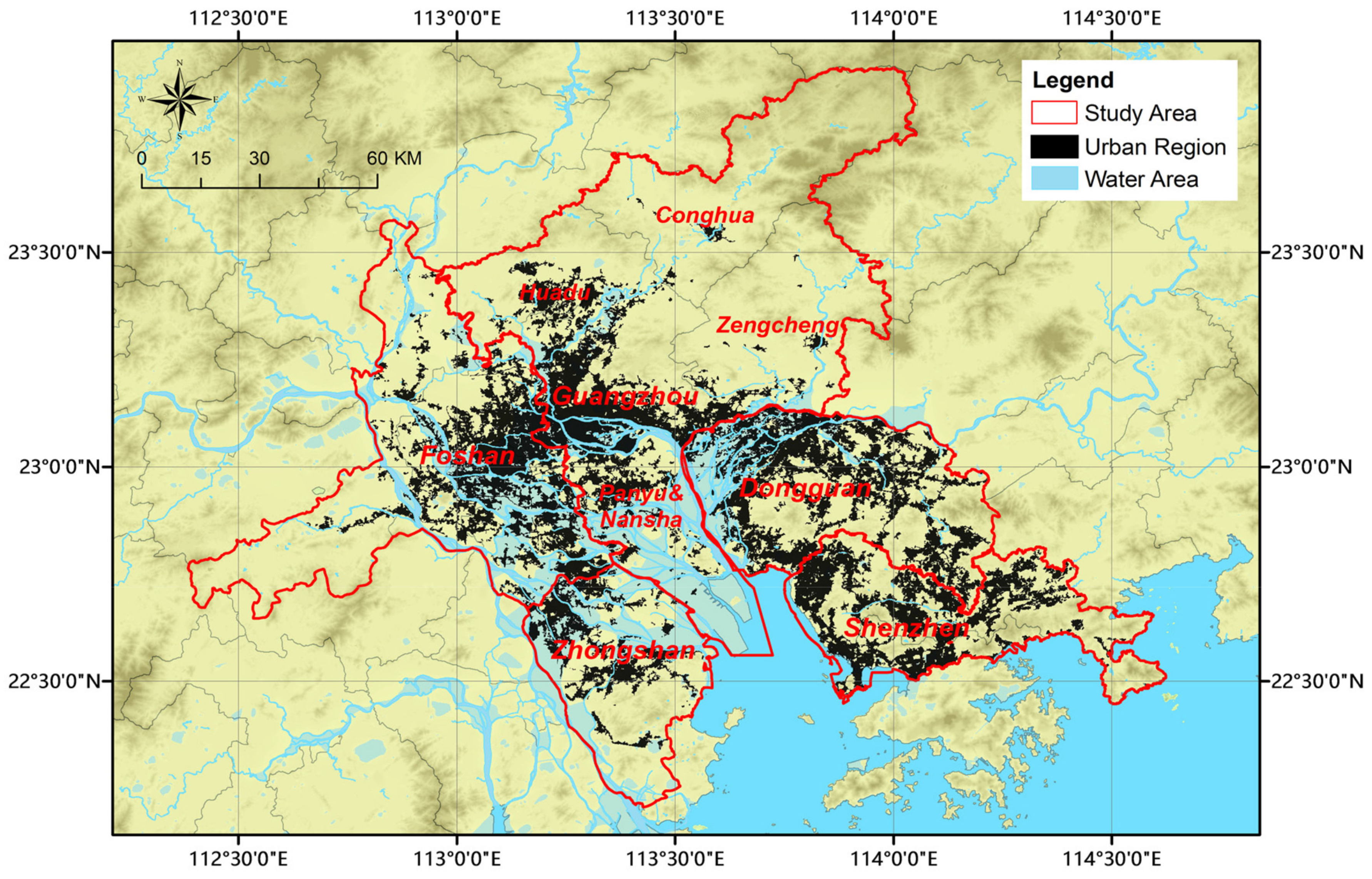
2.1. Study Area

The Pearl River Delta (PRD) is an emerging metropolitan area on the southern coast of China. The study area represents the core of the PRD, which is a typical large, complex urban growth area. This area comprises nine cities/districts, which include Guangzhou (GZ), Huadu (HD), Zengcheng (ZC), Conghua (CH), Foshan (FS), Zhongshan (ZS), Shenzhen (SZ), Dongguan (DG), Panyu, and Nansha (PN) (Figure 1). The growth characteristics of these cities vary because their economic structures and natural conditions are distinctive [21,22,23]. This area has experienced significant gross domestic production growth and unprecedented land-use changes in the last three decades [24]. Many land-related problems have been identified, including rapid urban sprawl, agricultural land loss, water pollution, soil erosion, and an increase in the magnitude and frequency of flooding [25]. The problems confronted in the PRD may soon be found in other rapidly-growing regions in developing countries [26,27].

A single Landsat Thematic Mapper (TM) image (no. 122-44 in the Reference System of China Remote Sensing Ground Station) nearly covers the nine cities and districts. Only some corners of Conghua, Shenzhen, and Zhongshan fall outside the scene. The use of a single image makes the research technically simpler, as it does not require creating an image mosaic.

2.2. Land-Use Data Processing

Three sets of cloud-free TM images were used in this study. These images were acquired on 13 October 1990, 14 September 2000, and 2 November 2009, respectively. Land-use classification was applied to each TM image. These images were radiometrically and geometrically corrected before the classification. Firstly, the dark-object subtraction (DOS) method was used to minimize the influences of weather and light conditions on land-use classification using the dark subtract tool of ENVI 5.1 [28]. Secondly, these images were geometrically corrected according to ground control points. The total RMS error of the geometric correction was controlled to less than 0.5 pixels. These corrected images were then classified using a series of techniques, including object-based supervised classification, manual editing, and intensive field labeling with GPS. The classification error rate for built-up land-use identified by field checking is about 3.11–8.97%.

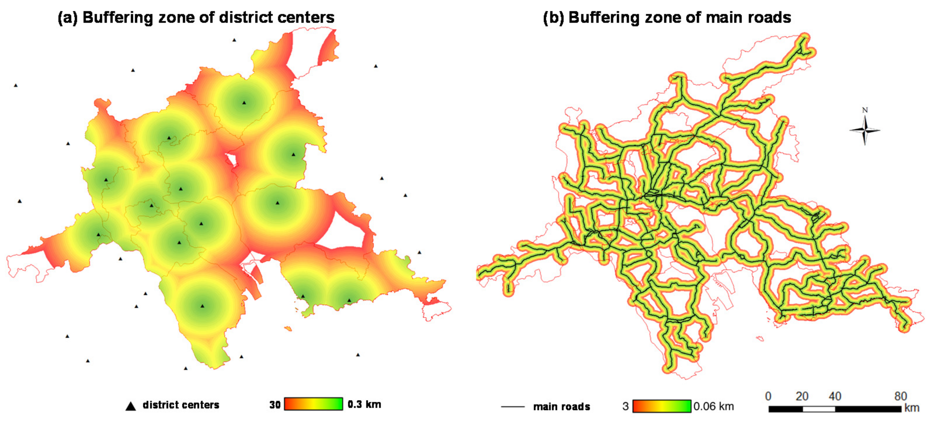
2.3. Indicators for Measuring Urban Growth

A large volume of research has been devoted to the study of urban growth [5,29,30] and many indices for measuring sprawl have been developed [22,31]. In this study, three indicators that are most related to CA modeling were selected to measure urban sprawl in the study area: growth rates, landscape expansion types, and spatial dependence.

• Growth Rate

The simpler land-based measures of sprawl are growth rate and the percentage change in land-use area [32,33]. The growth rate reveals the amount of available land converted to built-up land-use, while the percentage increase normalizes urban growth rates from initial built-up land-use areas. Growth rate (M_ue) can be defined using Equation (1):

$$M_{ue}=\frac{△U_i}{△t\times TL{A}_i}\times 100\%$$

(1)

where $△t$ is the study period, $△U_i$ is the increasing area of urban land use during the study period, and TLA_i is the initial urban land use area.

• Landscape Expansion Type

Landscape-expansion process analysis is used in urban-growth-measurement research and aims to understand the complex relationships between patterns in urban landscape change [34]. Urban landscape expansion involves three main types of spatial patterns: infilling growth, edge-expansion, and outlying growth. Other patterns can be regarded as variants or hybrids of these three basic forms [35,36,37].

LEI is used to identify patterns in new growth patches: (1) for infilling growth, the buffer zone of the new patch is mostly occupied by the old patch; (2) for edge-expansion growth, the buffer zone is mixed with vacant land (or other landscapes) and the old landscape; and (3) for outlying growth, the buffer zone is composed exclusively of vacant land. The LEI for a new patch can be evaluated using Equation (2):

$$LEI=100\times \frac{A_o}{A_o+A_v}$$

(2)

where LEI is the landscape expansion index for a newly grown patch, A_o is the intersection between the buffer zone and occupied land, and A_v is the intersection between the buffer zone and vacant land. The value of LEI varies between 0 and 100. When LEI ≥ 50, the newly-grown patch is identified as an infilling patch; when 0 < LEI < 50, the new patch is identified as edge-expansion; and when LEI = 0, the new patch is identified as outlying. A detailed description and calculation tool of LEI can be available at http://www.geosimulation.cn/LEI.html.

• Growth Spatial Dependence

The distance of land from city centers and roads is crucial for land zoning. Existing urban areas and roads are important spatial variables when building a land-use-change simulation model. As a result, analyzing the new growth patch’s spatial dependence is necessary when studying urban growth and its effect in the CA model.

Similar to the buffering procedure used by Xu et al. [38], Schneider [39] and Shi et al. [40], the newly-developed urban patch polygons were overlaid with a hundred buffer zones at 0.3 km from district centers (Figure 2a) and fifty buffer zones at 0.06 km from main roads (Figure 2b). These buffer zones were used to extract and calculate the area of the newly developed urban patch in each buffer ring. A line chart was then produced for each study city and the period to show the city center and road dependence of new growth patches.

2.4. Logistic CA Urban Growth Simulation Model

A logistic CA model was selected for the study’s urban growth simulation. The logistic CA is simple to define and convenient to calibrate using sampling data [41]. The methodology used here would be similar if the calibrating method were replaced by other data-mining methods, such as ANN-CA [42] and genetic CA [43]. The logistical model can be used to evaluate the development probability of non-urban land converting to urban land for simulating urban growth dynamics [41]. The development probabilities of urban CA are subject to change according to a series of urban growth related factors. The development probability of logistic CA can be calculated as Equation (3):

$$s_{ij}^t=\frac{\exp \left(z^t\right)}{1+\exp \left(z_{ij}^t\right)}=\frac{1}{1+\exp \left(-z_{ij}^t\right)}$$

(3)

where $s_{ij}^t$ is the development probability for cell ij at time t, $z_{ij}^t$ is a combined assessment score for development suitability ($z_{ij}^t=a_0+a_1{x}_1+\dots +a_m{x}_m+\dots +a_M{x}_M$), $a_0$ is a constant, $x_m$ is a spatial (physical) variable representing a driving force for urban growth, and $a_m$ is the parameter (weight) associated with variable $x_m$.

The above combined score $s_{ij}^t$ only addresses global factors in terms of proximity variables. However, urban growth is influenced by interactions at local levels, as well as global levels. Moreover, some spatial constraints can be incorporated to reflect the site conditions that also affect urban growth. By integrating all these geographical factors, the probability for development is further revised as Equation (4) [17]:

$$p_{ij}^t=\left(1+{\left(-\ln \gamma \right)}^{\alpha }\right)\times s_{ij}^t\times f\left({\Omega }_{ij}^t\right)\times co{n}_{ij}$$

(4)

where $\gamma$ is a stochastic factor ranging from 0 to 1, $\alpha$ is a parameter to control the stochastic degree, $f({\Omega }_{ij}^t)$ is the built-up land intensity in the neighborhood of ${\Omega }_{ij}$, which is calculated by Equation (5), and $co{n}_{ij}$ is the total constraint score ranging from 0 to 1:

$$f({\mathrm{\Omega }}_{ij}^t)=n/N$$

(5)

where n is the number of cells of built-up area in the neighborhood of ${\Omega }_{ij}$, N is the total number of cells in the neighborhood of ${\Omega }_{ij}$.

Finally, $p_{ij}^t$ is compared with a threshold value to determine if a non-urbanized cell will be converted into an urbanized cell at each iteration of the simulation as Equation (6):

$$S_{ij}^{t+1}=\{\begin{array}{cc}Converted,\hfill & p_{ij}^t\ge Q_{land}\\ NonConverted,& p_{ij}^t<Q_{land}\end{array}$$

(6)

where $S_{ij}^{t+1}$ is the state (non-urbanized or urbanized) of cell ij at next time (t + 1) and Q_land is a threshold value that is related to the amount of land conversion.

The threshold (Q_land) is estimated using observational data or an exogenous growth model to predict built-up land demand. This value can be chosen such that the total number of converted cells will be equal to the real number calculated from the observed remote sensing data.

In the following experiments, we use a figure of merit (FoM) [44] and Kappa index [45] to assess the accuracy of simulation results. The FoM measurements in this study were derived from overlays of the reference map of the initial time, the reference map of the subsequent time, and the prediction map for the subsequent time. This indicator focuses on change (the cells urbanized during the study period) instead of predicting persistence. FoM is a ratio ,which is calculated by Equation (7), where the numerator is the intersection of the observed change and predicted change while the denominator is the union of the observed change and predicted change [46]. The FoM can range from 0%, meaning no overlap between observed change and predicted change, to 100%, meaning perfect overlap between observed change and predicted change. A land change simulation model is acceptable when its performances is better than Null model that predicts pure persistence (no change between the map of the initial time and prediction map for the subsequent time) [47]. Pontius had compared 13 land change model applications with Null model [46]. Among the 13 applications, he found that, when the FoM is larger than 0.21, the model has a satisfactory predictive ability (better than the Null model).

$$\text{Figure of merit}=\mathrm{B}/\left(\mathrm{A}+\mathrm{B}+\mathrm{C}+\mathrm{D}\right)$$

(7)

where A is the area incorrectly predicted to persist, B is the area correctly predicted to change, C is the area incorrectly predicted to wrong land-use type, and D is the area incorrectly predicted to change.

A Kappa index was employed by many land use change studies to assess the accuracy of the results [21,45,48,49]. The Kappa index is calculated as Equation (8):

$$\mathrm{Kappa}=\frac{\mathrm{M}{\sum }_{i=1}^r{x}_{ii}-{\sum }_{i=1}^r\left(x_{i+}\ast x_{+i}\right)}{M^2-{\sum }_{i=1}^r\left(x_{i+}\ast x_{+i}\right)}$$

(8)

where $x_{ii}$ are the elements on the main diagonal of the error matrix, $x_{i+}$ is the sum of the ith row of the error matrix, and $x_{+i}$ is the sum of the ith column of the error matrix.

3. Results and Discussion

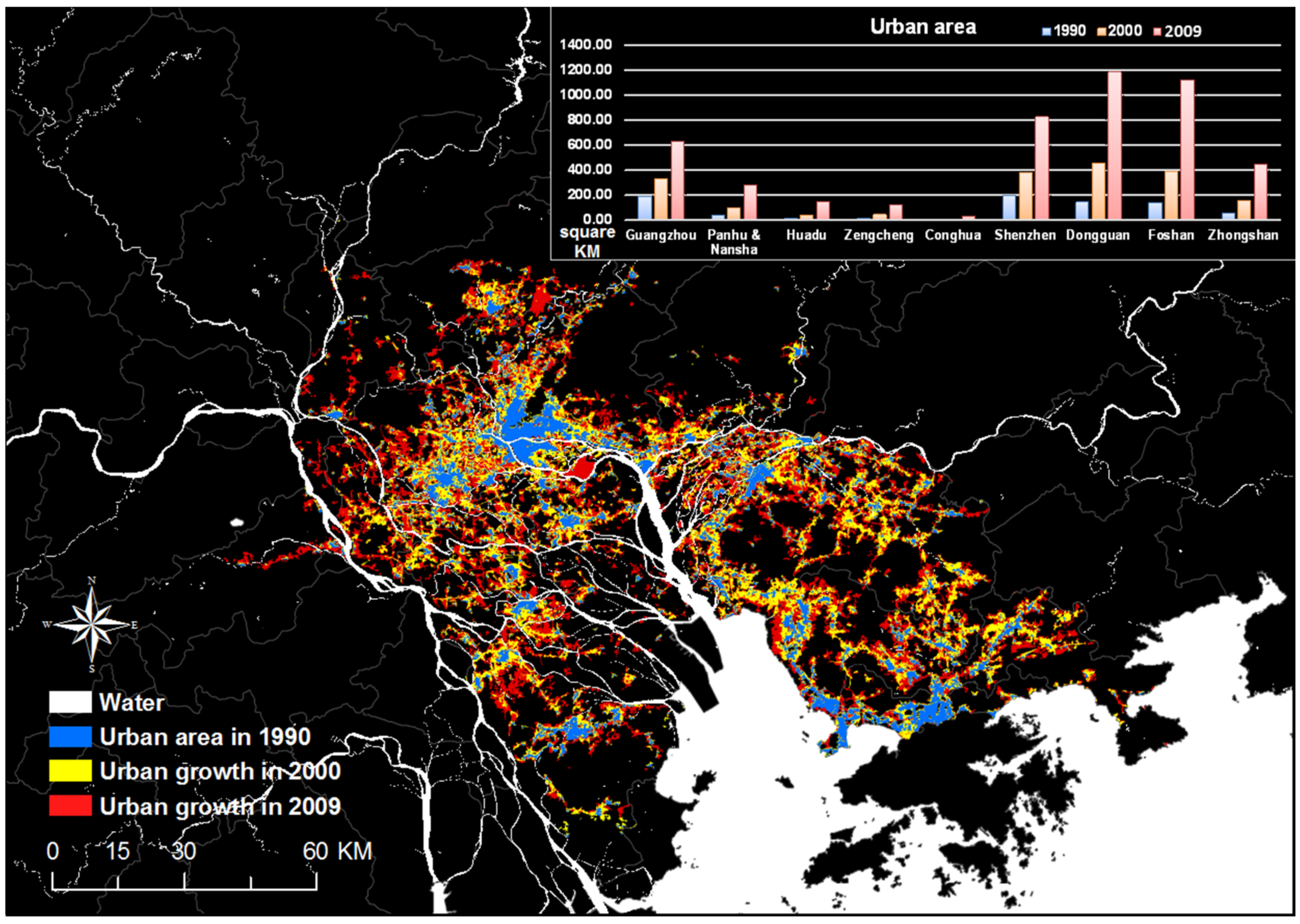
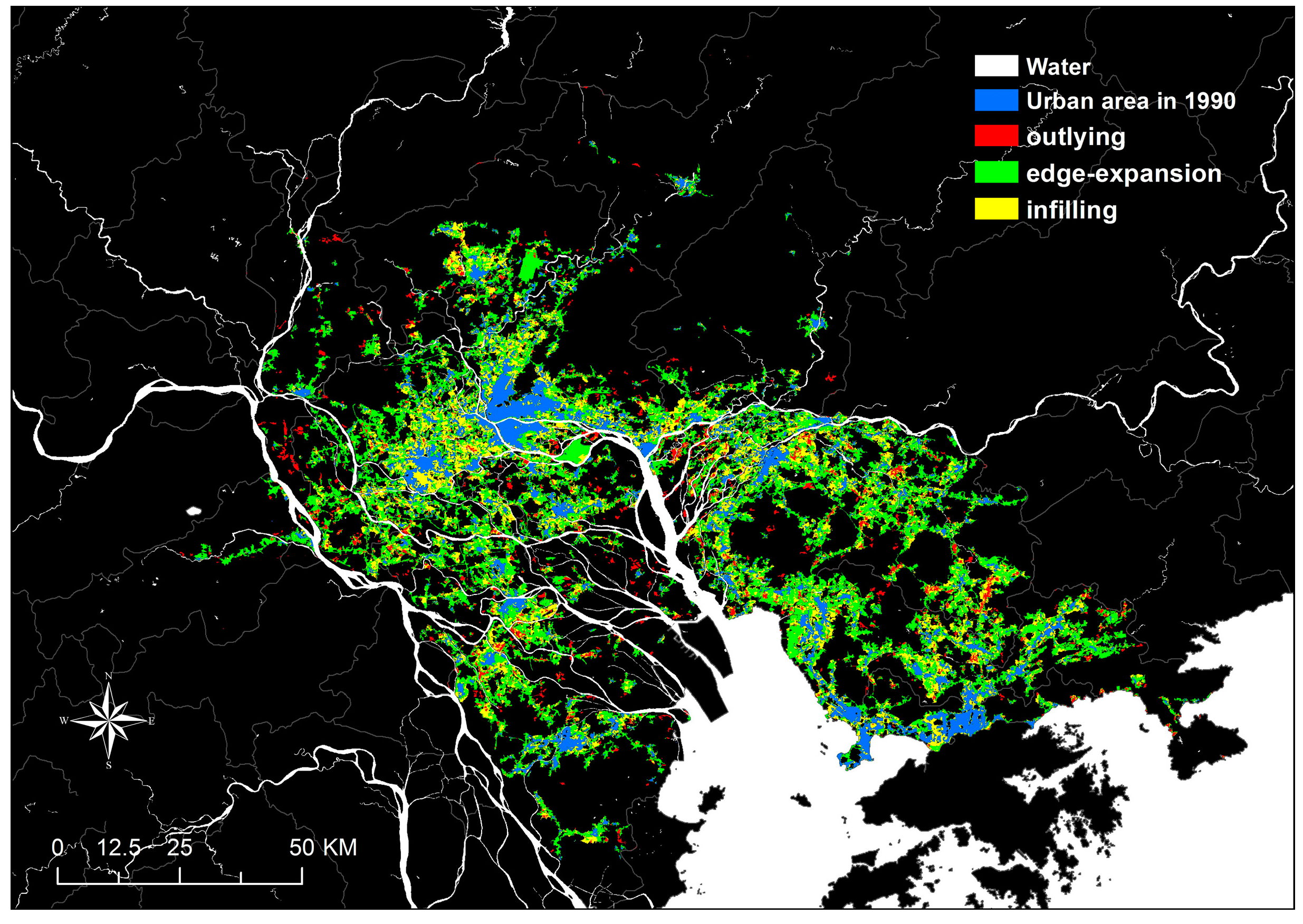
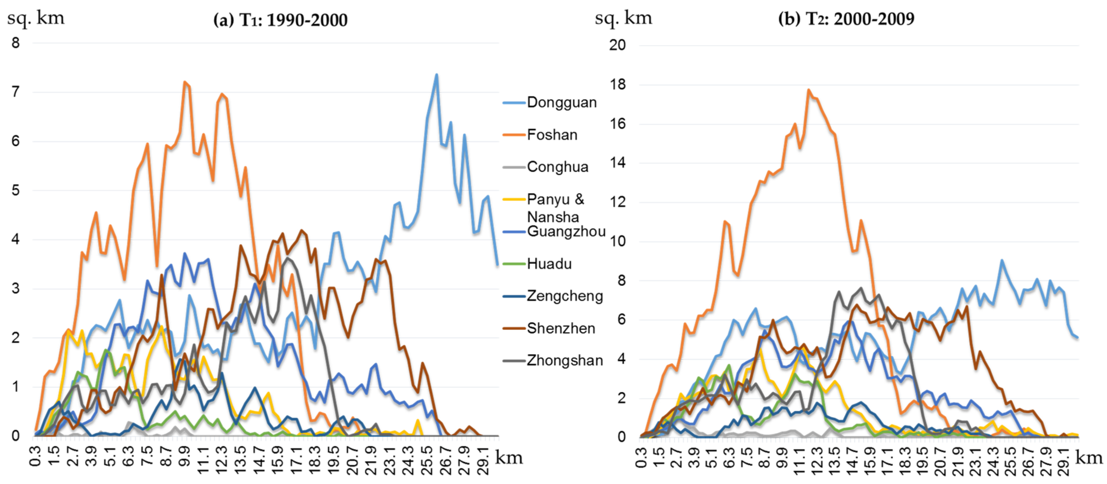
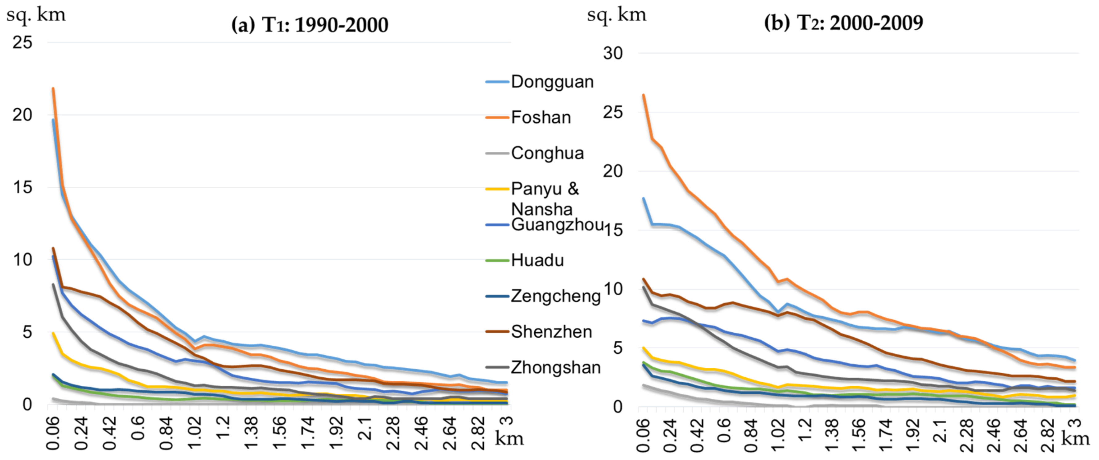
3.1. Urban Growth Measurement

• Growth Rate

The study period is divided into two periods (T1: 1990–2000 and T2: 2000–2009). According to the land-use classification of the study area, the growth ratio is calculated using Equation (2). During the study period, the study area experienced rapid urban area expansion, increasing from 790.52 km² to 4803.00 km². Figure 3 shows the urban growth during the period 1990–2009, with the annual urban growth ratio ranging from 2.52% to 21.43%.

As shown in Figure 3, the variation of each district’s urban area is different. The detailed data of built-up area and annual growth rate can be found in

Table 1. Annual built-up area growth number and growth rate of the nine cities over two periods.

No.	Period	1990–2000 (T1)		2000–2009 (T2)
	Region	Growth Area (km2)	Growth Rate (%)	Growth Area (km2)	Growth Rate (%)
1	Dongguan	313.05	21.43	724.35	17.53
2	Foshan	244.31	16.89	736.20	21.03
3	Conghua	2.12	2.52	19.87	20.99
4	Panyu & Nansha	64.28	16.42	181.01	19.44
5	Guangzhou	139.39	7.20	299.41	9.99
6	Huadu	27.72	17.40	108.04	27.50
7	Zengcheng	30.42	20.03	76.99	18.76
8	Shenzhen	182.11	9.28	447.84	13.16
9	Zhongshan	95.30	15.53	290.07	20.58

. According to the table, Dongguan and Foshan are growing quickly during T1 and T2. Both districts have the largest increase in built-up areas among the study area. The growth area (2.12 km²) and growth rate (2.52%) of Conghua during T1 is the lowest among all of the districts. However, the rate of Conghua is higher in T2 because Conghua is a satellite city of Guangzhou and its urbanization started late. The growth rates of Panyu and Nansha, Huadu, Zengcheng, and Zhongshan are similar, ranging from 15% to 20%. The growth rates of Guangzhou and Shenzhen are low because their urbanizations started early and they are developed regions. The growth rate of Zengcheng is also ranges from 15% to 20%, but its annual growth area is small.

• Landscape Expansion (Urban Growth) Types

The LEI was calculated for each new growth patch according to Equation (3). The buffer zones of the new urban patches were created by using a constant distance of 1 m.

Figure 4 shows the spatial distribution of three different urban growth types in the two periods.

Table 2. Growth type ratios of nine districts for periods T1 and T2.

Period	T1: 1990–2000			T2: 2000–2009
District	Outlying	Edge-Expansion	Infilling	Outlying	Edge-Expansion	Infilling
GZ	9.29%	74.78%	15.93%	2.02%	37.39%	60.59%
PN	16.14%	73.32%	10.54%	6.81%	59.24%	33.96%
HD	18.62%	78.63%	2.75%	5.29%	47.17%	47.54%
ZC	6.89%	86.75%	6.36%	4.16%	42.60%	53.24%
CH	3.08%	87.83%	9.09%	10.70%	60.76%	28.54%
SZ	10.93%	72.44%	16.62%	3.26%	50.22%	46.51%
DG	20.16%	71.00%	8.84%	2.61%	46.96%	50.44%
FS	12.42%	71.80%	15.78%	5.27%	48.31%	46.43%
ZS	18.93%	73.21%	7.86%	5.53%	56.32%	38.14%

shows the ratio of three urban growth types in different districts for the two periods. The urban landscape shows distinct growth patterns in different periods. During T1 (1990–2000), urban growth was dominated by edge expansion in most of the districts. However, outlying growth ratios are high in Panyu and Nansha, Huadu, Conghua, Shenzhen, Dongguan, Fashan, and Zhongshan, exhibiting a disordered and scattered pattern. Although infilling growth was also identified in the period, it was much less common, occurring only in the city proper. During T2 (2000–2009), fewer new outlying patches were found, while edge expansion and infilling growth became dominant (GZ, HD, ZC, and DG). However, edge expansion had decreased. Infilling growth intensified around district centers in some developed districts. Meanwhile, outlying growth increased, and edge expansion became dominant in Conghua because Conghua’s rapid urbanization began during this period.

• Growth Spatial Dependence

The newly developed urban patch polygons were overlaid with district-center (Figure 2a) and major-road (Figure 2b) buffer zones to calculate the spatial dependence of urban growth. The line charts in Figure 5 and Figure 6 show the district-center dependence and the road dependence of the newly developed urban patches. The X-axis is the distance from the district centers or roads, and the Y-axis is the area of the newly developed urban land during the study periods.

As shown in Figure 5 and Figure 6, the spatial dependence of each district’s new-growth built-up areas varies. In T1 (1990–2000), the new growth of urban land in Guangzhou, Zengcheng, and the new growth urban land of Shenzhen and Foshan were mainly grouped around district centers. The new growth urban land of Dongguan was mainly grouped around multiple centers, and these centers tend to connect with each other along the major road network. There are two reasons that Dongguan has this spatial dependence: (1) Guangzhou and Shenzhen, which are adjacent cities of Dongguan, have more influence than does Dongguan’s center; (2) the main source of the economy is the manufacturing industry, and the products need to be exported by road. Meanwhile, new development mainly took place along major transportation networks in most study districts, except Guangzhou, Huadu, and Conghua. During T2, district-center dependence is more notable (Figure 5b). There is dependence on major roads in all districts except Guangzhou and Conghua.

3.2. Urban Growth Simulation

The experiment seeks to explore CA simulation results that are calibrated with sample datasets from different districts. Logistic CA were applied to nine districts, simulating the urban growth process over two periods. Logistic CA uses global interaction and local interaction to address urban area dynamics. Global interaction (or development probability) is a function (Equation (3)) of proximity factors (distance to the district centers, distance to major roads), which is calibrated through a logistic regression. Local interaction is a function ($f({\Omega }_{ij}^t)$) of neighboring land-use types (the amount of built-up land in the neighborhood). The importance of proximity factors and neighborhood effects to urban simulations has been extensively discussed [7,17,41,50,51].

In the experiments, a 30 m × 30 m cell (pixel) was set as the basic analysis unit of the CA model. A total of 328 new growth sites were investigated for the period T1. Within these sites, a total of 3211 samples were randomly extracted. A total of 312 new growth sites were also identified for the period T2. These sites randomly yielded a total of 2109 pixels as the sample data. The samples were divided into 18 combinations according to the district and period. Development probability ($s_{ij}^t$) was calibrated using a logistic regression model for each combination. The dependent variable is binary (whether the land use is a built-up area) and independent variables, include the distance to the district centers and the distance to major roads, land elevation (DEM), and slope. Configuration of the neighborhood (${\Omega }_{ij}$) used a 3 × 3 neighborhood, and the threshold value (Q_land) was set to 0.8. Figure 7 displays the FoM and Figure 8 show the Kappa index in nine districts during the two periods. These figures clearly show that the FoM (ranging from 0.25 to 0.40) are high and satisfactory in GZ, SZ, and DG. The FoM (around 0.20) are low in CH and ZC. The reasons for the change in FoM for different districts and periods will be discussed in Section 3.3. The Kappa indices of each district are better than the Kappa of the Null model and range from 0.50 to 0.65 for the simulation of urban growth (excepting DG in T1) in the two periods. This range of Kappa means the consistency of the reference map and the prediction map is moderate or substantial, and the Kappa values are close with other studies [17,21,42,43,48] on CA modeling of the urban dynamics over the PRD areas.

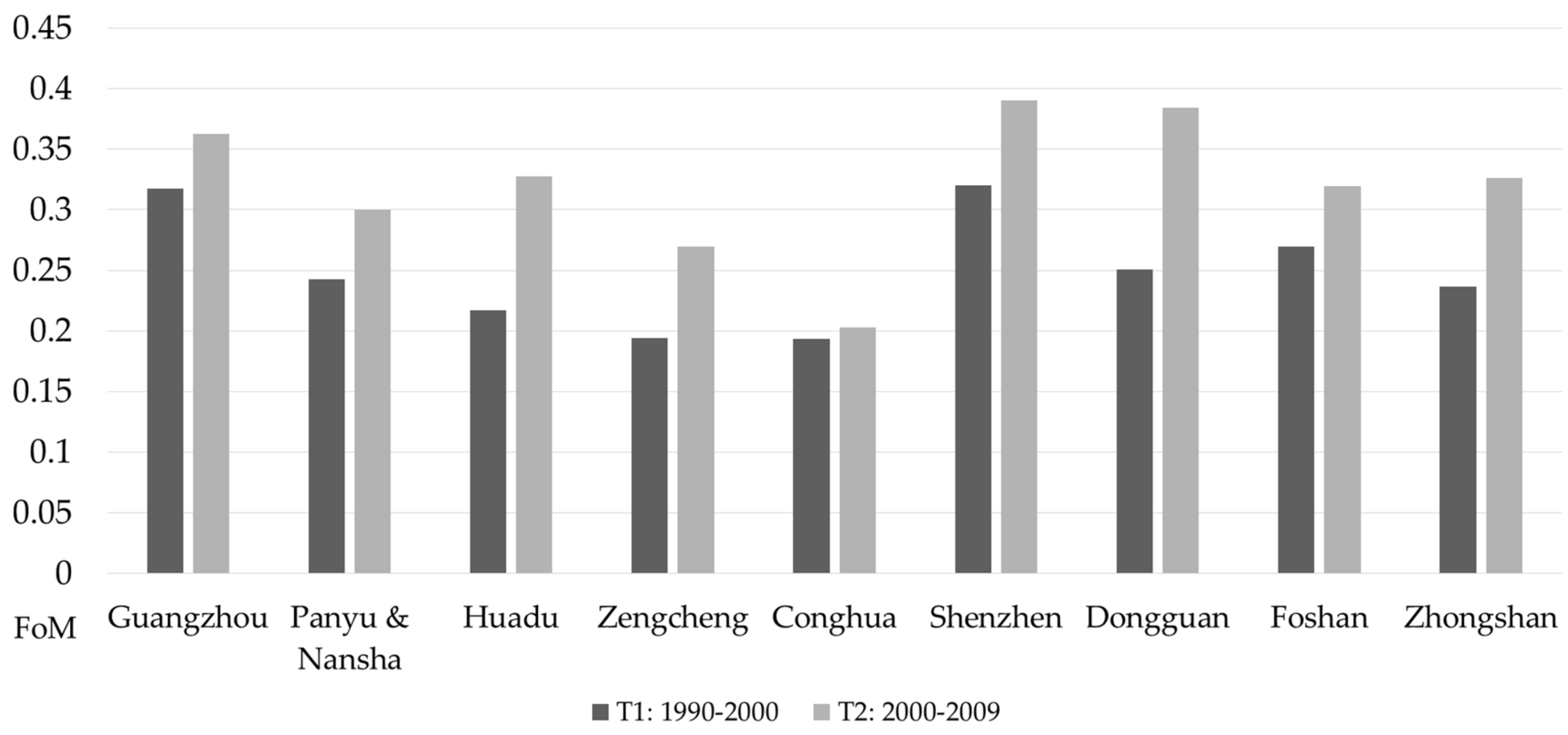
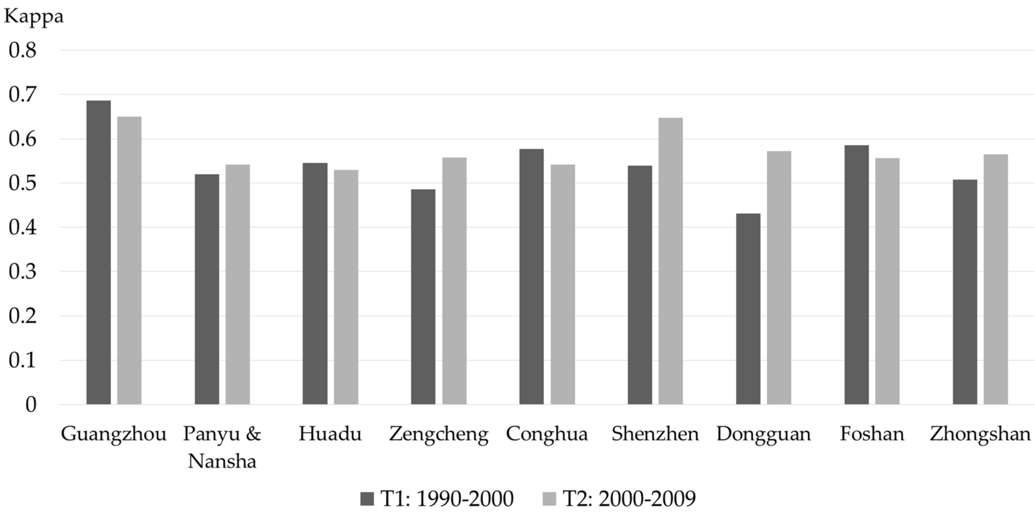
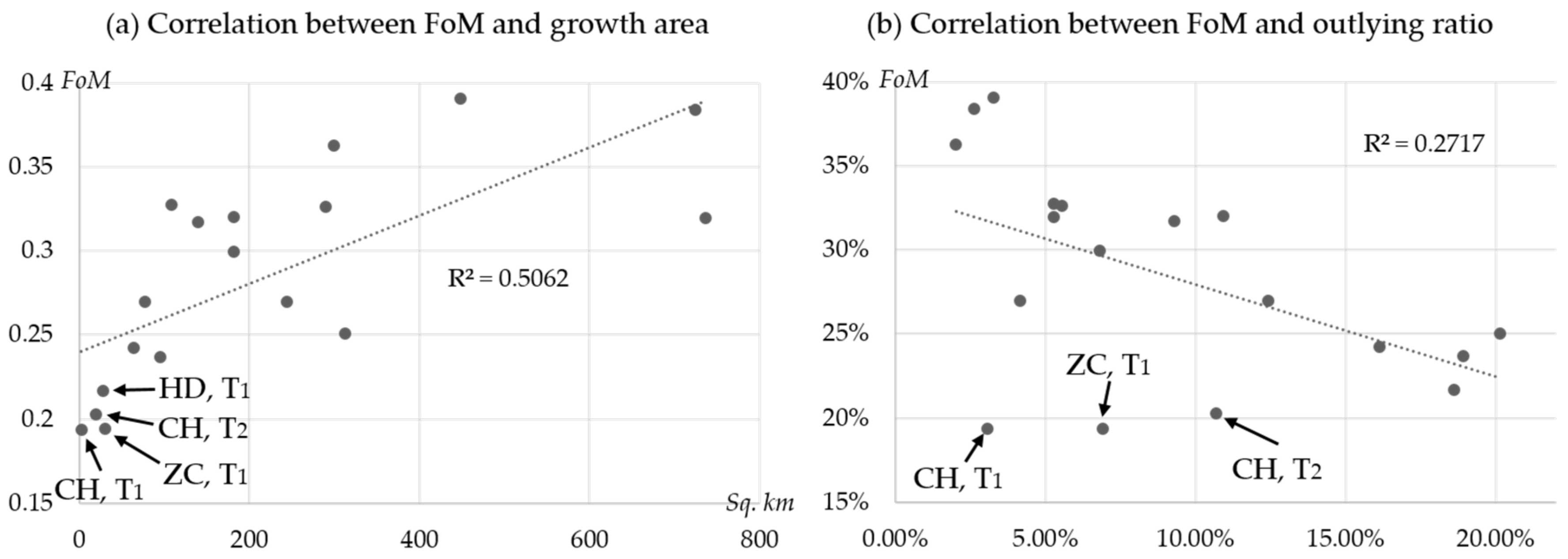
3.3. Expansion Type Ratio and Spatial Dependence Play a Key Role in CA Model Applicability

In the real-world situation, the new growth urban land is affected by many factors, which include some artificial factors such as the aspiration of the city authorities, urban planners, or investors. This is especially obvious in China. As a result, predicting the location of a few new growth patches is difficult. CA can be used to model the possibility and the location of the whole region. As shown in Figure 9a, if the quantity of the new growth areas is low, the randomization of the growth location is increased and the performance of the CA is decreased. In our case study, we find that there is a positive correlation between the growth rate and CA mode performance.

CA is a neighborhood-based model. As a result, a traditional CA model (such as logistic CA) is only applicable to edge expansion and infilling growth patches. Figure 9b clearly demonstrates that logistic CA performance is sensitive to the ratio of the outlying growth type. The performance of logistic CA tends to decrease when the ratio of outlying expansion increases (negative correlation between FoM and the “outlying ratio”). There are three cases (CH T1, ZC T1, and CH T2) that can be found in the figure showing that their outlying ratios are low while the CA models’ performance is poor. This is because the growth area quantities of these cases are low.

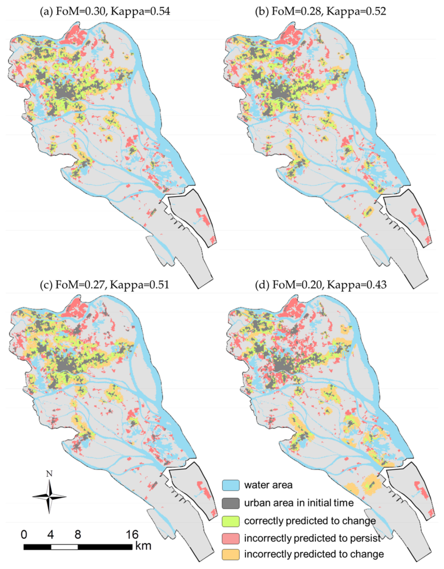
3.4. Domain Adaption of the CA Model

The urban-growth characteristics of each district vary, even when they belong to the same metropolitan area. The logistic CA model and other technical, data-mining land-use-change models require sample collection from the study area to calibrate the model. Hence these types of land-use-change models are not applicable to large regions that contain districts with different growth characteristics. Furthermore, samples collected from cities with similar growth characteristics can be used to calibrate a new land-use-change model. Additional experiments were implemented to test this hypothesis.

The aim of these experiments was to test whether the samples collected in other districts could be used to simulate the target district. The target district was set to Panyu and Nansha during the period 2000–2009. Four logistic CA models were built with different data sets. The data sets included samples collected from PN during T2 (D1), ZC during T2 (D2), PN during T1 (D3) and DG during T2 (D4). The growth characteristics of the four urban growth processes are shown in

Table 3. The growth characteristics of four trained data sources.

Trained Data Set	Data Source	Growth Area (km2)	Outlying Ratio	District Center Dependence	Major Road Dependence
D1	PN, T2	181.01	6.81%	Single center (4.0–14.0 km)	Low
D2	ZC, T2	76.99	4.16%	Single center (7.0–16.0 km)	Low
D3	PN, T1	64.28	16.42%	Multi-center	Low
D4	DG, T2	724.35	2.61%	Multi-center	High

.

The final simulated patterns of urban growth for Panyu and Nansha were obtained using these four models. The simulation patterns are shown in Figure 10. The areas in green were correctly simulated, while those in yellow (persistence simulated as change) and red (change simulated as persistence) were falsely simulated. The CA model calibrated with D1 is a reference pattern. We found that calibrating CA with D4 performed much poorer (the FoM and Kappa are the lowest in four cases) than calibrating CA with D2 and D3 (Figure 10b–d). We also found that the simulation result of the model calibrated with D4 has similar growth characteristics with DG T2. The new growth urban land is mainly grouped around multiple centers, and these centers tend to connect with each other along the major road network.

According to Table 3, although the source of D1 and D3 are in the same district, the difference of growth characteristics between source districts of D1 and D2 is less obvious than the difference between source districts of D1 and D3. The model that was calibrated with D2 can reach 94.3% performance (FoM) of the reference model. It is acceptable in application. The low growth characteristics diversity is the main reason why samples from other similar districts can be used to calibrate CA models.

4. Conclusions

Land-use-change models (such as the CA model) are powerful tools for studying and simulating the spatio-temporal and dynamic process of urban growth. Any land-use-change modeling requires decisions to be made, such as choosing the best-fit statistics for use during the calibration process. A preliminary study of urban-growth characteristics before building a land-use-change model is an important but often neglected step. Our results demonstrate how different growth characteristics impact on the overall performance of an urban land-use-change model.

According to our case studies, the performance quality of logistic CA tends to increase with an increased area of new growth and decrease with an increased ratio of outlying expansion. Traditional logistic CA is not applicable in three situations: (1) the urban growth process with a low growth area or high ratio of outlying expansion; (2) a large region that includes several districts/cities with different growth characteristics; and (3) a long period where the urban growth trend of the study area is shifting. Spatial dependence (such as proximity to district centers and major transportation networks) of the new growth patch plays a key role in CA model reusability. We can use samples from different districts to calibrate the CA model if these districts have similar growth characteristics.

We suggest that growth-characteristic analyses be conducted with each application such that the variability in map output can be assessed and incorporated into the interpretation of results with an acceptable level of confidence. Furthermore, the traditional logistic CA is reusable when applied to cities with the same growth characteristics. When the model needs to be applied to cities with different growth characteristics, we suggest using another technique (such as knowledge transfer or ensemble modeling) to improve the domain adaptive ability of the CA model. Future studies should also examine how other exogenous forces, such as land-use policies, are related to the urban-growth dynamic process and land-use-change modeling performance. These patterns reveal an interesting fact: the falsely simulated patches are usually situated in more remote areas. Future efforts are required to improve the simulation accuracy in these remote areas.

References

1. Brueckner, J. Urban growth models with durable housing: An overview. In Economics of Cities Theoretical Perspectives; Cambridge University Press: Oxford, UK, 2000. [Google Scholar]
2. Burchell, R.W.; Shad, N.A.; Listokin, D.; Phillips, H.; Downs, A.; Seskin, S.; Davis, J.S.; Moore, T.; Helton, D.; Gall, M. The Costs of Sprawl-Revisited; Tcrp Report 39; National Academy Press: Washington, DC, USA, 1998. [Google Scholar]
3. Downs, A. How America’s Cities Are Growing: The Big Picture. Brook. Rev. 1998, 16, 8–12. [Google Scholar] [CrossRef]
4. Ewing, R. Is Los Angeles-Style Sprawl Desirable? J. Am. Plan. Assoc. 1997, 63, 107–126. [Google Scholar] [CrossRef]
5. Johnson, M.P. Environmental impacts of urban sprawl: A survey of the literature and proposed research agenda. Environ. Plan. A 2001, 33, 717–735. [Google Scholar] [CrossRef]
6. Hua, L.; Tang, L.; Cui, S.; Yin, K. Simulating urban growth using the sleuth model in a coastal peri-urban district in China. Sustainability 2014, 6, 3899–3914. [Google Scholar] [CrossRef]
7. Verburg, P.H.; Soepboer, W.; Veldkamp, A.; Limpiada, R.; Espaldon, V.; Mastura, S.S. Modeling the spatial dynamics of regional land use: The clue-s model. Environ. Manag. 2002, 30, 391–405. [Google Scholar] [CrossRef] [PubMed]
8. Silva, E.A.; Clarke, K.C. Calibration of the SLEUTH urban growth model for Lisbon and Porto, Portugal. Comput. Environ. Urban. 2002, 26, 525–552. [Google Scholar] [CrossRef]
9. Parker, D.C.; Manson, S.M.; Janssen, M.A.; Hoffmann, M.J.; Deadman, P. Multi-agent systems for the simulation of land-use and land-cover change: A review. Ann. Assoc. Am. Geogr. 2003, 93, 314–337. [Google Scholar] [CrossRef]
10. Veldkamp, A.; Lambin, E.F. Predicting land-use change. Agric. Ecosyst. Environ. 2001, 85, 1–6. [Google Scholar] [CrossRef]
11. Wolfram, S. Cellular automata as models of complexity. Nature 1984, 311, 419–424. [Google Scholar] [CrossRef]
12. White, R.; Engelen, G. The use of constrained cellular automata for high-resolution modelling of urban land-use dynamics. Environ. Plann B 1997, 24, 323–343. [Google Scholar] [CrossRef]
13. Clarke, K.C.; Gaydos, L.J. Loose-coupling a cellular automaton model and gis: Long-term urban growth prediction for San Francisco and Washington/Baltimore. Int. J. Geogr. Inf. Sci. 1998, 12, 699–714. [Google Scholar] [CrossRef] [PubMed]
14. Li, X.; Yeh, G.O. Urban simulation using principal components analysis and cellular automata for land-use planning. Photogramm. Eng. Remote Sens. 2002, 68, 341–352. [Google Scholar]
15. Wu, J.; David, J.L. A spatially explicit hierarchical approach to modeling complex ecological systems: Theory and applications. Ecol. Model. 2002, 153, 7–26. [Google Scholar] [CrossRef]
16. Li, X.; Yeh, A.G.-O. Data mining of cellular automata’s transition rules. Int. J. Geogr. Inf. Sci. 2004, 18, 723–744. [Google Scholar] [CrossRef]
17. Li, X.; Liu, Y.; Liu, X.; Chen, Y.; Ai, B. Knowledge transfer and adaptation for land-use simulation with a logistic cellular automaton. Int. J. Geogr. Inf. Sci. 2013, 27, 1829–1848. [Google Scholar] [CrossRef]
18. Longley, P.A.; Mesev, V. On the measurement and generalisation of urban form. Environ. Plan. A 2000, 32, 473–488. [Google Scholar] [CrossRef]
19. Franck, G.; Wegener, M. Die Dynamik Räumlicher Prozesse; Raumzeitpolitik: Opladen, Germany, 2002; pp. 145–162. [Google Scholar]
20. Rajan, S.; Ghosh, J.; Crawford, M.M. An active learning approach to hyperspectral data classification. IEEE Trans. Geosci. Remote Sens. 2008, 46, 1231–1242. [Google Scholar] [CrossRef]
21. Liu, X.; Ma, L.; Li, X.; Ai, B.; Li, S.; He, Z. Simulating urban growth by integrating landscape expansion index (lei) and cellular automata. Int. J. Geogr. Inf. Sci. 2014, 28, 148–163. [Google Scholar] [CrossRef]
22. Cheng, F.; Geertman, S.; Kuffer, M.; Zhan, Q. An integrative methodology to improve brownfield redevelopment planning in chinese cities: A case study of futian, shenzhen. Comput. Environ. Urban 2011, 35, 388–398. [Google Scholar] [CrossRef]
23. Li, X.; Yeh, G.O. Analyzing spatial restructuring of land use patterns in a fast growing region using remote sensing and gis. Landsc. Urban Plan. 2004, 69, 335–354. [Google Scholar] [CrossRef]
24. Lu, S.; Guan, X.; He, C.; Zhang, J. Spatio-temporal patterns and policy implications of urban land expansion in metropolitan areas: A case study of Wuhan urban agglomeration, Central China. Sustainability 2014, 6, 4723–4748. [Google Scholar] [CrossRef]
25. Yeh, G.O.; Li, X. Economic transition, urban sprawl and agricultural land loss in the Pearl River Delta, China. Habitat Int. 1999, 23, 373–390. [Google Scholar]
26. Lambin, E.F. Modelling and monitoring land-cover change processes in tropical regions. Prog. Phys. Geogr. 1997, 21, 375–393. [Google Scholar] [CrossRef]
27. Murdiyarso, D. Adaptation to climatic variability and change: Asian perspectives on agriculture and food security. Environ. Monit. Assess. 2000, 61, 123–131. [Google Scholar] [CrossRef]
28. Chavez, P.S., Jr.; Kwarteng, A.Y. Extracting spectral contrast in landsat thematic mapper image data using selective principal component analysis. Photogramm. Eng. Remote Sens. 1988, 55, 339–348. [Google Scholar]
29. Squires, G.D. Urban Sprawl: Causes, Consequences and Policy Responses; Urban Institute Press: Washington, DC, USA, 2002; pp. 1–22. [Google Scholar]
30. Nechyba, T.J.; Walsh, R.P. Urban sprawl. J. Econ. Perspect. 2004, 18, 177–200. [Google Scholar] [CrossRef]
31. Li, X.; Chen, Y.; Liu, X.; Li, D.; He, J. Concepts, methodologies, and tools of an integrated geographical simulation and optimization system. Int. J. Geogr. Inf. Sci. 2011, 25, 633–655. [Google Scholar] [CrossRef]
32. Kasanko, M.; Barredo, J.I.; Lavalle, C.; Mccormick, N.; Demicheli, L.; Sagris, V.; Brezger, A. Are european cities becoming dispersed?: A comparative analysis of 15 European urban areas. Landsc. Urban Plan. 2006, 77, 111–130. [Google Scholar] [CrossRef]
33. Tsai, Y.H. Quantifying urban form: Compactness versus ‘sprawl’. Urban Stud. 2005, 42, 141–161. [Google Scholar] [CrossRef]
34. Schröder, B.; Seppelt, R. Analysis of pattern–process interactions based on landscape models—overview, general concepts, and methodological issues. Ecol. Model. 2006, 199, 505–516. [Google Scholar] [CrossRef]
35. Forman, R.T.T. Some general principals of landscape and regional ecology. Landsc. Ecol. 1995, 10, 133–142. [Google Scholar] [CrossRef]
36. Ellman, T. Infill: The cure for sprawl. Ariz. Issue Anal. 1997, 146, 7–9. [Google Scholar]
37. Wilson, E.H.; Hurd, J.D.; Civco, D.L.; Prisloe, M.P.; Arnold, C. Development of a geospatial model to quantify, describe and map urban growth. Remote Sens. Environ. 2003, 86, 275–285. [Google Scholar] [CrossRef]
38. Xu, X.U.; Song, Y.I.; Banks, S.P. On the dynamical behaviour of cellular automata. Int. J. Bifurc. Chaos 2007, 19, 1147–1156. [Google Scholar] [CrossRef]
39. Schneider, M.D. Examining the role of urban form in shaping peole’s accessibility to opportunities: An exploratory spatial data analysis. J. Transp. Land Use 2008, 1, 89–119. [Google Scholar]
40. Shi, Y.; Sun, X.; Zhu, X.; Li, Y.; Mei, L. Characterizing growth types and analyzing growth density distribution in response to urban growth patterns in peri-urban areas of lianyungang city. Landsc. Urban Plan. 2012, 105, 425–433. [Google Scholar] [CrossRef]
41. Wu, F. Calibration of stochastic cellular automata: The application to rural-urban land conversions. Int. J. Geogr. Inf. Sci. 2002, 16, 795–818. [Google Scholar] [CrossRef]
42. Li, X.; Yeh, A.G.-O. Neural-network-based cellular automata for simulating multiple land use changes using gis. Int. J. Geogr. Inf. Sci. 2002, 16, 323–343. [Google Scholar] [CrossRef]
43. Yang, Q.S.; Li, X. Calibrating urban cellular automata using genetic algorithms. Geogr. Res. 2007, 26, 229–237. [Google Scholar]
44. Pontius, R.G., Jr.; Millones, M. Death to kappa and to some of my previous work: A better alternative. Int. J. Remote Sens. 2011, 32, 4407–4429. [Google Scholar]
45. Congalton, R.G. A review of assessing the accuracy of classification of remotely sensed data. Remote Sens. Environ. 1991, 37, 35–46. [Google Scholar] [CrossRef]
46. Pontius, R.G., Jr.; Boersma, W.; Castella, J.C.; Larose, T.; Clarke, K.; Nijs, T.D.; Dietzel, W.; Boersma, C.; Duan, Z.; Fotsing, E.; et al. Comparing the input, output, and validation maps for several models of land change. Ann. Reg. Sci. 2008, 42, 11–37. [Google Scholar]
47. Maar, M.; Gzik, D.; Larose, T. Comparison of the structure and accuracy of two land change models. Int. J. Geogr. Inf. Sci. 2005, 19, 745–748. [Google Scholar]
48. Liu, X.; Li, X.; Liu, L.; He, J.; Ai, B. A bottom-up approach to discover transition rules of cellular automata using ant intelligence. Int. J. Geogr. Inf. Sci. 2008, 22, 1247–1269. [Google Scholar] [CrossRef]
49. Chen, Y.; Li, X.; Liu, X.; Ai, B.; Li, S. Capturing the varying effects of driving forces over time for the simulation of urban growth by using survival analysis and cellular automata. Landsc. Urban Plan. 2016, 152, 59–71. [Google Scholar] [CrossRef]
50. White, R.; Engelen, G. Cellular automata and fractal urban form: A cellular modelling approach to the evolution of urban land-use patterns. Environ. Plan. A 1993, 25, 1175–1199. [Google Scholar] [CrossRef]
51. Clarke, K.C.; Hoppen, S.; Gaydos, L.J. A self-modifying cellular automaton model of historical urbanization in the san francisco bay area. Environ. Plan. B 1997, 24, 247–261. [Google Scholar] [CrossRef]
Figure 1. Study area and urban region in 2009.
Sustainability 09 00796 g001
Figure 2. Buffering zone of district centers (a) and buffering zone of main roads (b).
Sustainability 09 00796 g002
Figure 3. Consistency of urban land use over the study period.
Sustainability 09 00796 g003
Figure 4. Spatial distribution of three urban growth types.
Sustainability 09 00796 g004
Figure 5. Spatial dependence of urban growth from district centers over two time periods. (a) Period T1: 1990–2000 and (b) Period T2: 2000–2009.
Sustainability 09 00796 g005
Figure 6. Spatial dependence of urban growth from major roads over two time periods. (a) Period T1: 1990–2000 and (b) Period T2: 2000–2009
Sustainability 09 00796 g006
Figure 7. Figure of merit (FoM) of the simulation results for nine districts.
Sustainability 09 00796 g007
Figure 8. Kappa indices of the simulation results for nine districts.
Sustainability 09 00796 g008
Figure 9. Correlation between model performance and growth characteristics: (a) Correlation between FoM and growth area; (b) correlation between FoM and outlying ratio.
Sustainability 09 00796 g009
Figure 10. Simulation patterns of four cellular automata (CA) models: (a) CA calibrated with D1; (b) CA calibrated with D2; (c) CA calibrated with D3, and (d) CA calibrated with D4.
Sustainability 09 00796 g010