Article

Pan-European Calculation of Hydrologic Stress Metrics in Rivers: A First Assessment with Potential Connections to Ecological Status

by
Yiannis Panagopoulos
1,2,*,
Kostas Stefanidis
1,2,
Marta Faneca Sanchez
3,
Frederiek Sperna Weiland
3,
Rens Van Beek
4,
Markus Venohr
5,
Lidija Globevnik
6,
Maria Mimikou
1 and
Sebastian Birk
7,8
1
Center for Hydrology and Informatics, National Technical University of Athens, 15780 Athina, Greece
2
Hellenic Centre for Marine Research, Institute of Marine Biological Resources and Inland Waters, 19013 Anavissos Attikis, Greece
3
Stichting DELTARES, 177 Delft, The Netherlands
4
Department of Physical Geography, Faculty of Geosciences, Utrecht University Stichting DELTARES, 80115 Utrecht City, the Netherlands
5
Department of Ecohydrology, Leibniz-Institute of Freshwater Ecology and Inland Fisheries, 12587 Berlin, Germany
6
Faculty of Civil and Geodetic Engineering, University of Ljubljana, 1000 Ljubljana, Slovenia
7
Faculty of Biology, Aquatic Ecology, University of Duisburg-Essen, 45141 Essen, Germany
8
Centre of Water and Environmental Research, University of Duisburg-Essen, 45141 Essen, Germany
*
Author to whom correspondence should be addressed.
Water 2019, 11(4), 703; https://doi.org/10.3390/w11040703
Submission received: 3 March 2019 / Revised: 29 March 2019 / Accepted: 1 April 2019 / Published: 5 April 2019
(This article belongs to the Special Issue Hydrologic Modelling for Water Resources and River Basin Management)

Abstract

:
The hydrologic regime of a river is one of the factors determining its ecological status. This paper tries to indicate the present hydrologic stress occurring across European rivers on the basis of model integration. This results in a pan-European assessment at the resolution of the functional elementary catchment (FEC), based on simulated daily time-series of river flows from the model PCR-GLOBWB. To estimate proxies of the present hydrologic stress, two datasets of river flow were simulated under the same climate, one from a hypothetic least disturbed condition scenario and the second from the anthropogenic scenario with the actual water management occurring. Indicators describing the rivers’ hydrologic regime were calculated with the indicators of hydrologic alteration (IHA) software package and the river total mean flow and the relative baseflow magnitude over the total flow were used to express the deviations between the two scenarios as proxy metrics of rivers’ hydrologic alteration or hydrologic stress. The alteration results on Europe’s FEC-level background showed that Southern Europe is more hydrologically stressed than the rest of Europe, with greater potential for hydrology to be clearly associated with river segments of unreached good ecological status and high basin management needs.

1. Introduction

The hydrologic regime represents the primary driving force of river ecosystems as it determines the various characteristics of water flow over time (e.g., extent and duration of base flow or flooding), shapes the patterns of erosion and sedimentation, and influences the type and dynamics of the river channels, banks and floodplains [1]. The hydrologic regime affects water chemistry through processes of retention, dilution or concentration. By this, it constitutes the habitat template for the riverine biota. Hydrology is thus an indispensable component of riverine ecology, and anthropogenic alteration of the hydrologic regime entails ecological detriment [2].
Riverine hydrology is altered by humans in various ways [3,4]. At the local to regional scale, water abstraction, water diversion, water drainage and channelization modify the flow regime for the benefit of domestic, industrial or agricultural supply. In particular, dams represent one of the major anthropogenic disturbances of the rivers’ hydrologic regimes [5]. At the river basin scale, the water retention capacities are reduced by converting natural vegetation into land used for agriculture or urbanization. At the continental scale, patterns of precipitation and evaporation shift due to a changing climate, with important changes in climate extremes over time. These alterations impact on the riverine ecosystems and lead to changes in natural flows, including water scarcity or overabundance with implications for ecological status and ecosystem services [6,7].
However, full understanding of the effects of hydrologic alteration is still not available [8]. On the one hand, this relates to the intricate features of riverine hydrology covering the elements of timing, magnitude, duration and frequency, all of which are integral components of the ecosystem [9]. On the other hand, this relates to the lack of comprehensive datasets, e.g., from stream gauges, precluding empirical cause-effect modeling. Data shortage applies in particular to records of unaltered, natural hydrologic regimes and especially in the densely populated and highly modified landscapes of Europe and elsewhere. These obstacles hamper scientific understanding in support of effective water and river basin management as, for instance, required by the European Water Framework Directive (WFD) [10].
In the absence of measured data, hydrologic effects on the riverine ecosystems can be investigated using flow regimes derived from hydrologic modeling. For the European context, various models are available that all follow a similar approach and can all reasonably estimate discharges at a continental scale, such as PCR-GLOBWB [11,12,13,14,15,16], LISFLOOD [17] or HYPE [18,19,20]. These models produce discharge outputs taking catchment management into consideration; thus, they allow for simulating river discharges under conditions modified by human activities (‘anthropogenic’), but can also predict riverine hydrology under least disturbed conditions (LDC) altered only slightly by humans [21]. LDC refers to the best available physical, chemical, and biological habitat conditions given today’s state of the landscape where the influence of human water management in the form of irrigation and reservoir management is excluded, and for which we have data available. These two model outputs (i.e., anthropogenic and least disturbed) enable comparisons between the modified and least disturbed river discharges, providing prerequisites to calculate quality ratios used in environmental assessment [22].
In this paper we have selected PCR-GLOBWB to demonstrate the application of a large scale hydrologic model deriving daily time-series of river discharges at high spatial resolution covering the entire European continent. The purpose was to analyze the time-series produced under two different scenarios to discover the deviations between them and assess the present hydrologic alteration (or ‘stress’) of European rivers. Hydrologic alteration was expressed using the indicators of hydrologic alteration [23] calculated for the two model outputs of anthropogenic and least disturbed conditions. The resulting ratio allowed for determining types of hydrologic stress occurring across European river basins, providing a first solid basis for future research on cause-effect modeling and catchment management at cross-basin and continental scale.

2. Materials and Methods

2.1. Method of Indicators of Hydrologic Alteration (IHA)

The indicators of hydrologic alteration (IHA) were originally proposed by Richter et al. [9] to assess the degree of hydrologic alteration caused by human intervention on rivers. The hydrologic parameters are computed with the use of a free software tool developed by The Nature Conservancy [23]. The tool has a user-friendly interface that needs daily time-series of river discharge as input. The IHA method has been updated with a new set of hydrologic parameters (called ‘E-flow components’ [24]), which categorizes river flows into low- and high-magnitude events. As a result, there are 70 hydrologic parameters (indicators) that can characterize the annual or intra- and inter-annual variability in water conditions, including the magnitude, frequency, duration, timing and rate of change of flows.

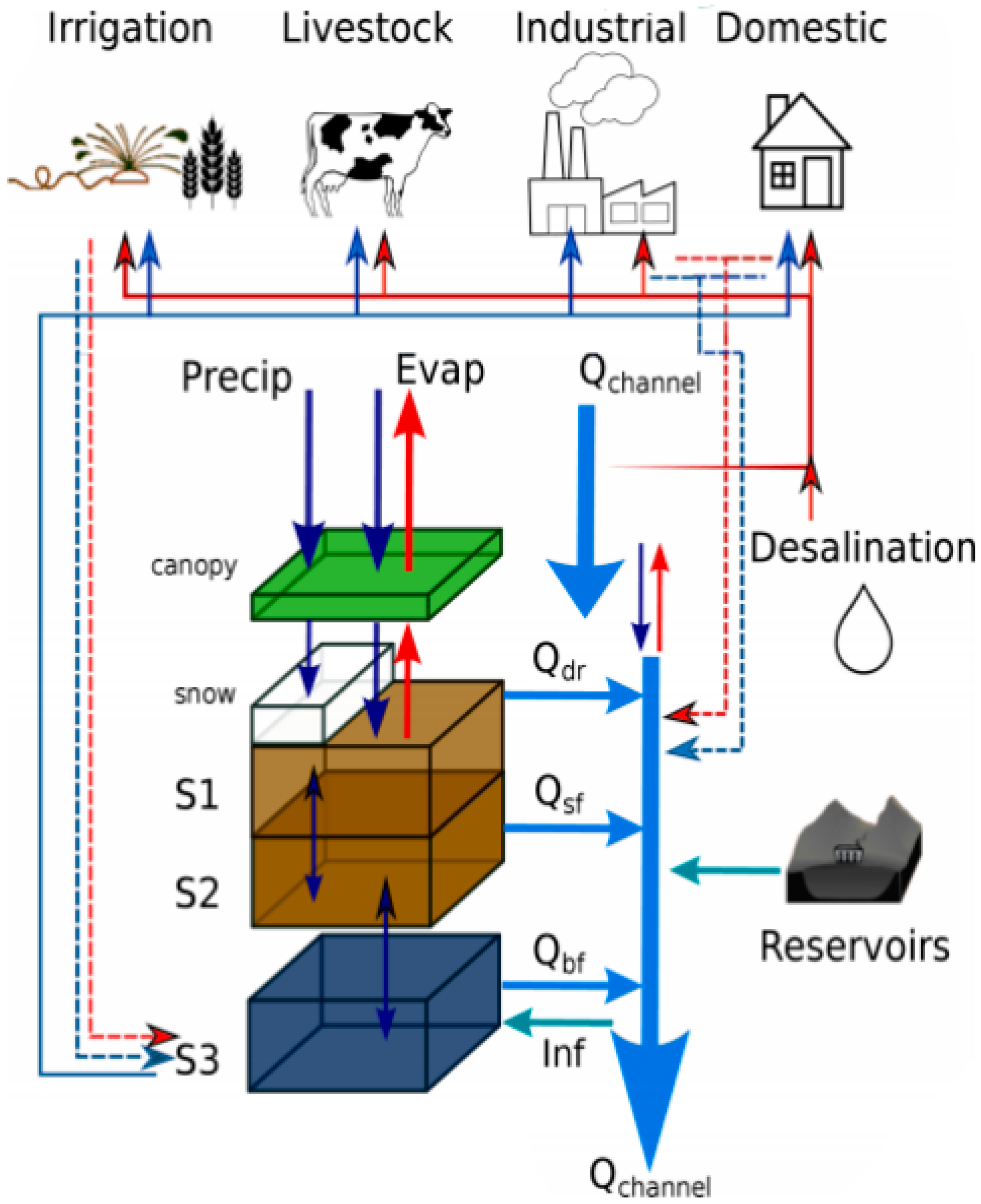
2.2. Hydrologic Data at European Scale—PCR-GLOBWB Modelled Data

The implementation of the IHA method at the European scale requires a continuous daily discharge dataset covering the whole of Europe. This can only be achieved with the use of simulated data. In this study we employed the global hydrologic model PCR-GLOBWB for the simulation of river flows and runoff for Europe. PCR-GLOBWB is essentially a “leaky-bucket” type of model applied on a cell-by-cell basis [13,14]. A spatial resolution of 5 arc minutes (≈10 km × 10 km at the equator) and a daily temporal resolution were used in this study. A schematic representation of PCR-GLOBWB (version 2.0), which has been applied in this study, is given in Figure 1. For each time step and cell, PCR-GLOBWB calculates water balance components. These include water storage in three vertical soil layers (0–5, 5–30 and 30–150 cm) and one underlying groundwater layer, as well as the water exchange between the layers (percolation, capillary rise) and between the top layer and the atmosphere (rainfall, evapotranspiration and snowmelt). Sub-grid variability is taken into account considering the variations of elevation, land cover, vegetation and soil. The total runoff of a cell consists of direct runoff (saturation excess surface runoff), non-infiltrating melt water, interflow (lateral drainage from the soil profile) and baseflow (groundwater runoff from the lowest linear reservoir). Simulated runoff was routed along the river network based on the simulated topological networks (STN30) [25]. Model parameterization was based on global datasets of soil properties, vegetation and geological information. Parameterization together with model evaluation (global validation) details have been presented in Van Beek et al. [13] and Sutanudjaja et al. [14].
PCR-GLOBWB simulations have been performed for the period 1960–2010, including the dynamic changes in climate occurring within this 50-y period. Hydrologic alteration assessments were based on 10-y simulations though, using the last decade of this period’s simulations (see Section 2.5).
As for the meteorological forcing, the monthly precipitation, monthly temperature and reference potential evaporation of CRU TS3.23 [26] were used. CRU TS3.23 has been constructed by interpolating historical observed station time-series to a global grid with a resolution of 0.5 degrees. Its quality highly depends on the availability of local station observations which is particularly high in North–Western Europe. As PCR-GLOBWB runs at daily resolution, the monthly fields of CRU TS3.23 forcing data were downscaled to daily values using the ECMWF ERA20C re-analysis from the European Centre for Medium-Range Weather Forecasts (ECMWF). Daily averages and totals were computed by combining the 6 h time steps of the re-analysis. The original spatial fields at 0.7° were assigned to the cells center and then spatially interpolated to the finer model grid of 0.5° (30 arc minutes). Precipitation was temporally downscaled by first applying a threshold of 0.1 mm day−1 to the ERA daily timeseries to estimate the number of rain days for ERA and remove drizzle. The amount of rainfall below this threshold was proportionally allocated to the rain days. After this, the CRU monthly rainfall sums and monthly average temperatures have been disaggregated to daily values based on the daily distribution in the ERA20C re-analysis (see Sutanudjaja et al. [14]).

2.3. Scenarios: Least Disturbed Condition and Anthropogenic

To address hydrologic stress in this study, hydrologic simulations were performed for two scenarios. One was the least disturbed conditions (LDC) scenario where no water use, irrigation, abstractions, industry or water/reservoir management are considered. For this scenario, only natural surface water bodies (e.g., rivers, wetlands and lakes) are included. This scenario represents least disturbed conditions because the land cover types do not represent pristine conditions, as unaltered by man, but are (similar to the anthropogenic scenario; see below) based on the map of Global Land Cover Characteristics Database version 2.0 [27] and MIRCA dataset for agricultural land cover types, which encompasses current land use conditions including crop lands, production forests and built-up areas, amongst others. A grid-cell contains different land cover classes but no land use/cover change throughout the simulation was considered: no land use information was available to simulate a scenario of pristine hydrologic conditions and we decided to maintain the land use map of 1960 and not to expand the irrigation areas, which would reflect increased human activities throughout the simulation period. Hence, all crop types under the LDC were modelled as rainfed.
In the anthropogenic scenario a grid-cell constituted up to five land cover classes: short natural vegetation, tall natural vegetation, surface water bodies (including reservoirs), and irrigated paddy and non-paddy crop types. For this scenario, areal extents of fractions of all land cover classes changed on yearly basis, particularly due to expansion of irrigated areas and progressive construction of dams/reservoirs, which were taken into account based on Zarfl et al. [28], supplementing previous data on reservoirs based on the GRAND database [29].
The anthropogenic differed from the LDC scenario in the sense that water use for industry, irrigation, domestic use and livestock could be abstracted from the surface and groundwater depending on availability and pre-defined groundwater abstraction limits. For the definition of water demand the model relies on global datasets that have specifically been developed to aggregate country statistics and localized information such as FAOSTAT and MIRCA2000 [30]. The PCR-GLOBWB model includes a water demand scheme to estimate irrigation water requirements. Irrigation water demand is calculated based on the crop composition (which changes per month and includes multiple cropping) and the irrigated area per cell. The scheme separately parameterized two different irrigated crop groups: paddy and non-paddy and their growing season defined based on the MIRCA2000 dataset [30]. The crop vegetation phenology and rooting depths were based on the Global Crop Model [31]. Based on these datasets, the fraction of the cell covered with the specific crop groups and their growing stage was defined. In case of non-paddy irrigation, water was applied whenever soil moisture falls below a pre-set value and then the soil column was replenished up to field capacity. In case of paddy irrigation, the water level was kept at a water depth of 5 cm above the surface until the late crop development stage (≈20 days) before the harvest. After that, no irrigation was applied anymore such that the water level is allowed to drop to zero under infiltration and evaporation [32]. The net irrigation demand is corrected for irrigation efficiency and losses for which country-specific loss factors have been obtained from Rohwer et al. [33] (for more details, see Wada et al. [32]). The quality of the estimated irrigation needs is depended on the source data. The MIRCA dataset, for example, is available at the 5 arc minutes resolution but the information content varies per country.
Other sectoral water demands, including those from livestock, industry and household, were compiled from several sources, e.g., Wint and Robinson [34] and FAOSTAT (http://faostat.fao.org/). The development of these historical sectoral water demand databases in PCR-GLOBWB was mainly based on the algorithm developed by Wada et al. [35] that considers many factors: trends in water demand are prescribed on an annual basis as a function of population, electricity demand and gross domestic product (GDP) per capita, which do show a strong relation with change in water use but are only proxy-estimators. The annual domestic water demand is re-distributed throughout the year on the basis of temperature. Domestic and industrial gross water demand was calculated from net water demand using a country specific recycling ratio (RC; gross demand = net demand/[1 − RC]), which is based on development stage or GDP per capita and additionally access to domestic water demand. This takes into account that much of the domestic and industrial water is not consumed but returned as surface water [32,35].
Livestock water demand was calculated by multiplying the number of livestock in a grid cell with its corresponding drinking water requirement, which is a function of air temperature. The gridded global livestock densities of cattle, buffalo, sheep, goats, pigs and poultry and their corresponding drinking water requirements were obtained from FAO [36] and FAOSTAT (http://faostat.fao.org/). A simple reservoir management scheme was implemented that applies to approximately 6000 man-made reservoirs worldwide. A release strategy was imposed on these reservoirs that aimed at passing the average discharge downstream, while maintaining reservoir levels between a minimum and maximum storage [32].
In general, water demand was simulated to determine water abstractions considering water availability. Both LDC and anthropogenic scenarios were projected with the climate of the period 2001–2010 (see Section 2.5), thus, differences in the two scenario outcomes were attributed to water use, irrigation and reservoir management. The demand was an external force and not influenced by the model conditions, yet the actual use is limited by the local water availability. Within the model, water for industry could be abstracted from ground- and surface water whereas return flows were always added to the surface water.
In the configuration of the model applied here, water can be abstracted from surface water and groundwater. The ratio between surface water and groundwater use is determined as a function of their relative abundance. Surface water withdrawal was ceased if river discharge fell below 10 % of the long-term average yearly discharge under naturalized flow conditions [37]. If the surface water amount was insufficient (most likely during summer) the model fell back on groundwater to meet the resulting gap. The amount of groundwater that can be abstracted was limited by the groundwater pumping capacity, which is based on data from the IGRAC GIS database. For urban areas, we rely on the data set of McDonald et al. [38] that states whether a surface water distribution infrastructure is available. Here, industrial and domestic water withdrawals are mainly taken from surface water before abstracting groundwater, otherwise groundwater is prioritized. For irrigation, we used the ratios supplied by Siebert et al. [39] in regions where they are said to be reliable. Within the PCR-GLOBWB abstraction scheme it was assumed that all the water demand is supplied from surface water and groundwater resources in the same cell.

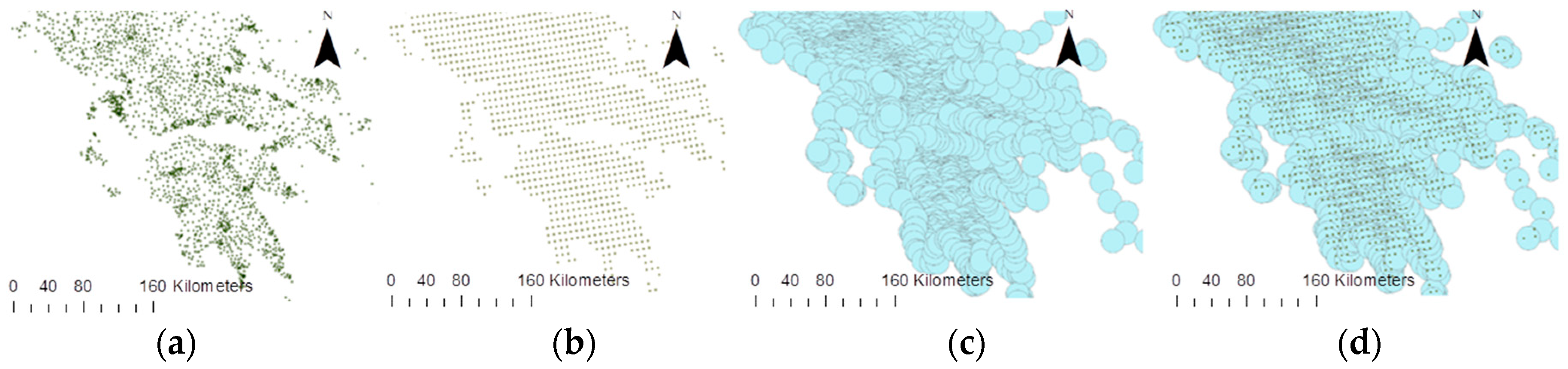
2.4. PCR-GLOBWB Data Allocation to Functional Elementary Catchments

The PCR-GLOBWB simulations resulted in two datasets of gridded daily discharges (m3/s). The first dataset represented the daily discharges for the anthropogenic scenario (i.e., baseline conditions), while the second dataset simulated daily discharges under the LDC scenario. The purpose of this second dataset was to simulate the hydrologic conditions in Europe under a status of minimal anthropogenic pressures on water arising from abstractions and water management modifications (including reservoir operations).
We assigned the gridded hydrologic data from PCR-GLOBWB to the 104,334 functional elementary catchments (FECs) of Europe, with an average area of ≈60 km2 [40], available in the database of the project MARS [41,42]. The FEC background layer was selected as the best hydrogeographical background layer at pan-European scale, available at the time of this research, being a robust mapping product of suitable resolution to capture the gridded information of the PCR-GLOBWB model. The gridded model output was transferred to FECs based on the closest neighboring distance and verification with the use of upstream drainage areas of grids and FECs. At first, the centroids of the FEC polygons were calculated and a new shapefile was produced as shown in Figure 2a. The share of the upstream area that corresponded to each FEC was matched with the FEC centroid objects. Next, a new shapefile of the centroids of the modelled raster cells was created (see Figure 2b). For each FEC’s centroid a buffer with a 15 km radius was created (see Figure 2c) and then intersected with the PCR-GLOBWB centroid shapefile to identify what cell centroids fall within the buffer area of each FEC’s centroid. This resulted in having several grid points in one FEC buffer (see Figure 2d). Then, for each case (FEC buffer) we selected the cell centroid for which the absolute difference between the FEC’s upstream area and grid cell’s upstream area was at a minimum. This allowed us to reduce the number of cases where a grid cell with a large upstream area was wrongly assigned to a neighboring but non-representative FEC (e.g., a small tributary). Finally, we checked the correspondence between the upstream areas of FECs and grid cells to ensure that a perfect match existed (1:1 line and R2 = ≈1). This whole process had also been executed by using the outlet-points of FECs instead of FECs’ centroids in an effort to identify the most suitable correspondence between FECs and grid cells. From the analysis we noticed that both approaches (FEC-centroids or FEC-outlet-points) resulted in highly comparable outcomes, with the FEC-centroids approach performing slightly better.

2.5. Calculation of Indicators of Hydrologic Alteration for Europe

Due to the extremely time- and effort-demanding IHA calculations for the whole of Europe at FEC-level we used daily PCR-GLOBWB time-series of only 10 years (10-y) in the present pan-European work, ranging from 2001 to 2010. The anthropogenic scenario was represented by the climate and anthropogenic activities of this period, while the LDC scenario was based on the land use and management described in Section 2.3 and the same climate (2001–2010) in order to be able to attribute changes to anthropogenic impacts (in terms of land use and water management). The 2 × 104,334 FEC-daily discharge datasets for the two scenarios were imported to the IHA software in groups of 1050 10-y daily time-series (1050 FECs) exploiting the batch import capability of the tool [23]. Each subset needed almost half of a working day to run. This short time-series length, however, could be restrictive for deriving representative statistical indices, especially with regard to hydrologic metrics related to extreme events that require the definition of a rather big return period. Given the necessity to reach a compromise, the 10-y length of the used time-series was considered as the optimum choice to explore potential hydrologic stress on the basis of shorter than normal time-series, which nevertheless could at least give reliable indication of the general hydrologic characteristics [43].
Seventy indicators were calculated by the IHA software from a time-series analysis. Among the general indicators calculated were the mean flow and number of zero flow days of the entire time-series, the Baseflow Index representing the entire time-series, which is defined as the seven day minimum flow (average)/mean annual flow of the year within which the seven day minimum flow occurs, as well as reversals, which are calculated by dividing the hydrologic record into “rising” and “falling” periods, with the number representing the times that flow switches from one type of flow (high or low) to the other [23]. Low and high flows have been determined first on a daily basis for the entire time-series, with the criterion of flow being below or above thresholds that correspond to percentiles predefined by the user (by default all flows greater than the 75th percentile of daily flows were high flows, all flows less than or equal to the 50th percentile of daily flows were low flows, and thresholds of flow rate were used to determine the type of daily flows for the intermediate values lying within the 50th to 75th percentiles). Further, extreme low and very high flows (small and large floods) were determined from the final sets of low and high flows respectively, with predefined percentiles or the definition of a return period [23]. An event was comprised of consecutive days of low or high flows and was ended on the day that the status changes from low to high and the opposite. The IHA indicators addressed the frequency, duration and severity of high and low flow events, while also giving the timing of the events and the 3, 7, 30, and 90 day minimums and maximums from moving averages of the appropriate length calculated for every possible period that is completely within a water year of the time-series.

2.6. Formulation of Hydrologic Stress Metrics

We quantified the hydrologic stress calculating ratios between the values of each hydrologic indicator derived from the anthropogenic scenario and the values of the respective indicators derived from the least disturbed condition (LDC) scenario (anthropogenic scenario over LDC scenario) for all FECs. This had the added benefit that any biases in the simulated flow were removed and comparison between locations became easier. If the value for a certain indicator was unity, it meant that there was no alteration between the anthropogenic model run and the LDC model run. If the ratio was above unity, the value of the hydrologic indicator for the anthropogenic scenario was higher than the LDC scenario, and if the ratio was below unity, the value of the hydrologic indicator for the anthropogenic scenario was lower than the LDC scenario. In fact, to eliminate the very insignificant changes between the two scenarios, the ‘no alteration’ class assigned to a ratio of unity was decided to contain all ratios within the small range 0.975–1.025 and the other two classes the rest of the FECs with a >2.5% increase or decrease in the hydrologic parameters between the two scenarios. All the >2.5% increases and decreases were included in the two respective alteration classes regardless the alteration intensity, as the purpose of this work was not to demonstrate various alteration magnitudes at a spatially detailed context. The three classes of ratios (1, >1 and <1) were mapped at the FEC level to show the areas with hydrologic alteration (either exceeding or falling below the LDC values) or no hydrologic alteration, respectively.
To facilitate the mapping analysis at the large-scale (multiple sites with flow time-series) we had to reduce the number of hydrologic indicators to be used to those that ensured a clear assessment of the nature of the hydrologic alteration. As many of the calculated IHA indicators were inter-correlated (e.g., duration and frequency), resulting in considerable information redundancy [44], we tested them for collinearity according to the variation inflation factor (VIF) criterion [45]; indicators with VIF > 7 were removed. Furthermore, we excluded all monthly outputs and the timing of events occurrence. On the one hand, it was not our purpose to analyze inter- or intra-annual hydrologic features and their changes in this assessment of hydrologic stress. On the other hand, these parameters have been proved to be of small reliability in similar studies [43]. Due to the short length of time-series used in this study (10 years), the indicators related to the extreme low flows or the frequency and duration of flood events were deemed to be biased [43]. They were thus not used in the pan-European mapping analysis. Against this background, we focused on the indicator results related to the magnitude of river flows, which is more sensitive to changes in water management and reliable in showing the alteration trend, regardless the simulation length. We considered that relying on the magnitude also reduces the influence of possible biases in the quantification of flows by the hydrologic model.

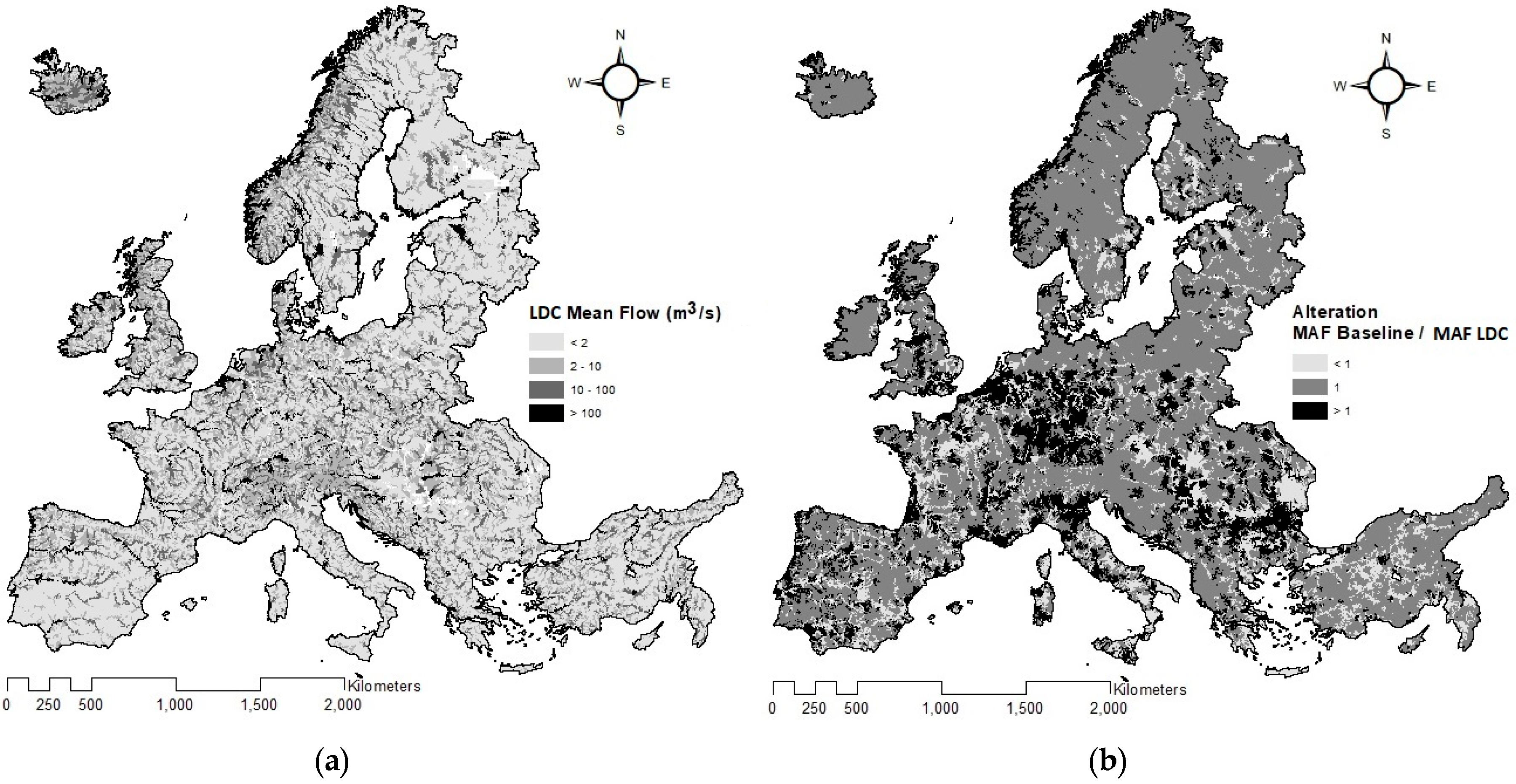
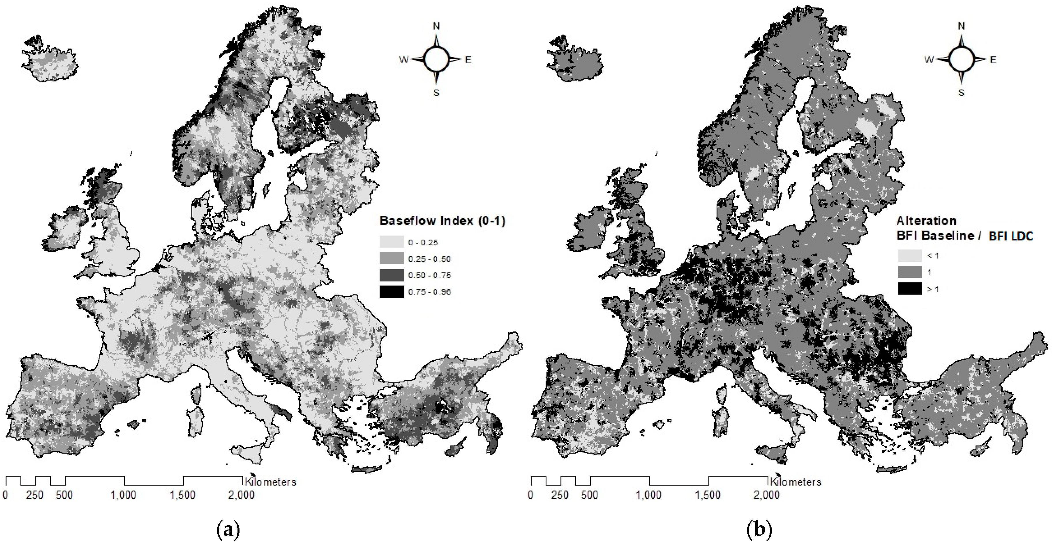
3. Results and Discussion

For this first assessment of hydrologic alteration at the European scale the use of the mean annual flow (MAF) and the baseflow index (BFI) provided very informative outputs from the IHA package implemented. In general, decreased MAF and BFI in the anthropogenic scenario from the LDC scenario corresponded to an added stress on water because either the total flow (and water availability) decreased or the baseflow component of total flow was reduced, with the latter being responsible for the preservation of water availability in the river throughout the year. Both indicators showed distinct patterns of hydrologic alteration across Europe (Figure 3 and Figure 4).
A clear reduction of annual river flows is indicated in Figure 3b by the <1 areas for parts of all the Mediterranean countries (Greece, Turkey, Spain, France, Italy) due to the modified water management and water abstractions occurring in the anthropogenic scenario. However, the alteration map of the figure shows that the average flow conditions were not influenced for most of the rest of Europe (ratio = 1), except a considerable part in Central Europe (mostly Germany and Northern Italy) and in South–Eastern Europe, where the ratio is greater than unity. The reduction of flows in the South is rather easy to interpret: irrigated crop areas added in the anthropogenic scenario were responsible for large amounts of water abstracted from water bodies and used by crops. The typical irrigation abstraction needed in the dry period of the year for the growth of a typical crop in Southern countries is around 500 mm of water, which is equivalent to 5000 m3/ha [46,47]. Water in PCR-GLOBWB was obtained either directly from rivers or from surface reservoirs and groundwater. The impact of groundwater depletion on river flows is well-known in Southern countries, resulting in poorer contribution to surface water hydrology as, due to the warm climate, this irrigated water becomes almost entirely crop evapotranspiration [47,48]. Given that irrigated agriculture mostly exists in the South, many rivers in the Mediterranean countries have been impacted negatively and this is considered the major factor for noticing significant areas with MAF ratios < 1. On the other hand, the areas with MAF ratios > 1 in Central and South–Eastern Europe show actual river discharges greater than the natural ones. This seems strange as human impact is commonly expected to influence water availability to the negative direction. The driver for this ‘positive’ direction is caused by groundwater abstractions for industrial water use, household water use and irrigation and the related return flows or losses to the surface water system that are included in the anthropogenic simulations. Water for industry and households can be abstracted from surface and groundwater but the release of the non-consumptive water use, i.e., the return flows, is always added to the hydrologic surface water network. A similar re-distribution of groundwater to surface water originates from irrigation where, especially in summer and in dry regions, a large share is taken from the groundwater and added to the top soil potentially leading to a minor runoff to the surface water. Near the Dutch–German border, Southern Germany, Italy and South–Eastern Europe we found areas with relatively high groundwater abstractions. Groundwater abstractions were highest around major cities, industrial areas and dry irrigated areas. According to Wada et al. [49] groundwater abstractions have increased substantially, especially in the second half of the past century. Since the 1990s this has contributed to a global increase of river flow discharging to the sea.
Moreover, water storage in reservoirs may locally increase the surface water availability, and both Central and South–Eastern Europe feature a high number of new dams and associated reservoirs [29]. According to the hydrologic model parameterization the construction of dams resulted in a number of new reservoirs and thus increased surface water extent, yet not all dams necessarily resulted in large upstream reservoirs. The increase in reservoirs’ actual evaporation was at most locations relatively small and local compared to the much more important role of groundwater abstractions. So the return flows resulting from groundwater abstractions did mainly increase river flows in several parts of Europe.
The BFI under the LDC scenario shows that aquifers play a key role in the streams’ total flow in Central and Northern Europe, enhancing long low flow events as already described above (Figure 4a). The higher the BFI, the greater the groundwater contribution is to streamflow. The highest BFI values were observed in Northern Europe, especially in Northern UK and Scandinavia but also in parts of Central and Southern Europe (e.g., Spain and Turkey) with values greater than 0.5 in many areas (Figure 4a). In other parts of Southern Europe, however, the BFI was below 0.5, with Italy for instance being entirely below 0.25. In general, the magnitude of the BFI depends on the topography and hydrogeology of catchments, including the temporal distribution of recharge, and can vary greatly across Europe.
What is more important here is the change of the index due to the simulation of the anthropogenic scenario (baseline; Figure 4b). The BFI was not altered due to abstractions for large parts of Europe, but decreased mostly in parts of the Mediterranean countries (ratio < 1). Similarly to the analysis of MAF, this is interpreted by the occurrence of considerable groundwater abstractions for irrigation that reduce groundwater levels and thus the volume of water, which aquifers can release to adjacent streams and rivers. Moreover, some areas in Central and Eastern Europe had greater BFI in the anthropogenic scenario, and this was observed almost in the same areas that also had greater MAF. We think that even in this case the driver is the same, namely the reservoir operations, industrial development and associated return flows that cause important water release to the hydrographic network in the Central European areas and the irrigation water returns in the South–Eastern areas. As a result of the permanent water release to the rivers, the minimum 7 day low flow conditions (which are considered in the calculation of BFI) increased, leading to an increased BFI compared to the LDC scenario. However, in such cases the resulting BFI should be interpreted with caution: The 7 day low-flow used for the calculation of the index cannot be solely attributed to aquifer’s contribution, but it may have artificially increased due to the point source discharges and other return flows to surface waters. This reduces the validity of the conceptual design of the index to describe flow conditions, specifically when BFI is increased compared to a reference condition (LDC scenario in our case). The mathematical expression of the BFI, having mean annual flow in the denominator, allows for ratios > 1 due to increased relative significance of the numerator (7 day lowest flow) which may have been increased due to constant releases from the dams or return flows.
The discussion above was based on our outcomes that the hydrologic indicators related to the magnitude of river flows (and especially with the average and low flow conditions) were the most informative in identifying hydrologic alteration or hydrologic stress. Other hydrologic indicators related to the frequency and duration of events did not change at all or changed only slightly from the reference conditions, but more importantly, they had limitations in this particular work. This is in line with the study of Vigiak et al. [43] who discussed the hydrologic indicator results calculated from the implementation of several models implemented in four European catchments. Their results showed that modelled flow magnitude indicators were generally reliable, whereas indicators for flow timing, duration, and rate of change were affected by large uncertainties. They also found that the impact of the period length on the accuracy of 120 indicators of hydrologic alteration quickly improved when the period of analysis increased from one to 15 years, with a minimum length of 20 years being recommended when occurrence of rare events is of interest (extreme flows, duration of low flows). Thus, their paper documents that prevalent weight should be given to those indicators that are more robust to quantify, such as long-term mean annual indicators, compared to indicators that are highly uncertain, such as those defined in relation to set thresholds.
Our work presented the hydrologic alteration through a general classification of the 104,334 FECs of Europe (see Figure 3 and Figure 4). One class contained the ‘no alteration’ results assigned to a ratio of 1, which in fact contained all ratios within the small range 0.975–1.025. The other two classes included the rest of the FECs with a >2.5% increase or decrease in the hydrologic parameters between the two scenarios. As explained in the methodology, all the >2.5% increases and decreases were included in the two respective alteration classes regardless the alteration intensity, as the purpose of this work was not to demonstrate various alteration magnitudes at a spatially detailed context. It should also be mentioned that in both the MAF and BFI results (Figure 3b and Figure 4b, respectively) there were a very few FECs (<1%) with a ratio extremely higher than unity or extremely close to zero. This is attributed either to extreme changes in management under the anthropogenic scenario or to possible model errors in those FECs. Given that these FECs were very few and were not geographically concentrated, they were not distinguished from the others on the maps but remained within the two alteration classes.
Regarding other hydrologic indicators derived from the IHA software package, there were interesting ones, although not informative. Starting with the characteristics of the low flow conditions across Europe, the total number of low flow days remained unaltered for the majority of the European area within the 10-y simulated periods of the LDC and the anthropogenic scenarios. This was expected because in both scenarios low flows were defined as all daily flows less than or equal to the 50th percentile of the whole daily time-series of each FEC. But between the two 10-y scenarios we also noticed that there were no considerable differences in the duration of low flow events (consecutive low flow days) across Europe. In Northern and North–Eastern Europe low flow events were the longest without particular difference between the two scenarios, while for all other, mainly the more Southern areas, low flow periods were shorter and increased very slightly in the anthropogenic scenario. Differences were so small (i.e., within the 2.5% deviation range) that they could not give us a clear indication of hydrologic stress. On the other hand, high flow events did not last more than a week on average in both Southern and Central Europe, but were much longer in Northern Europe reaching a month or more. However, similar to the low flow events, they could not reveal considerable alteration when compared between the two scenarios, with the calculated ratios being very close to unity.
Accordingly, the number of reversals, namely the changes in the type of flow (low/high) within the entire 10-y simulation period, did not change substantially from the LDC scenario under the anthropogenic scenario, and remained consistently lower (<<50 per year) in the Northern areas (longer events, fewer switches from low to high flows and vice-versa) than in the rest of Europe (>50 per year). Similarly, changes in the characteristics of the very high flow events were also of low significance all across Europe. But more importantly, they were calculated from non-representative frequencies and durations of the flood events occurring in the two scenarios. For example, large flood events were defined as the high flow events with a (minimum) 10-y return period, questioning its usefulness in our study, which used 10 years of length of the entire hydrologic time-series. Nevertheless, despite the above, no remarkable changes of the frequency and duration of the very high flow events all across Europe were expected between the anthropogenic and LDC runs in our constant-climate scenario study.
Those changes along with deviations of other hydrologic parameters would be more pronounced in a climate change scenario study where precipitation and temperature averages and extremes may change significantly. Future work can include holistic future world scenarios based on combinations of representative concentration pathways (RCPs) and shared socioeconomic pathways (SSPs), which represent future climate worlds with particular socioeconomic characteristics [50,51]. The RCPs refer to radiative forcing pathways that describe an emission trajectory and concentration by the year 2100, while the SSPs are defined as ‘reference pathways’ describing plausible alternative trends in the evolution of society and ecosystems. Such scenarios have been already produced and used in local analyses in the EU funded MARS project [52,53], and would be interesting to run and give rise to hydrologic alteration estimates at the European scale in the future.
Another issue worthy of discussion is related to the reliability of the model used and the present expressions and estimates of hydrologic alteration. Regarding the second, uncertainties may have been added both by the indicator definition [54], for example the BFI here, and the definition (and simulation) of the reference condition [43], the LDC in this work which was inevitably formulated based on some assumptions and simplifications. More criticism is often expected on the first though, namely the model used in the analysis and its prediction capacity, especially when implemented at a very large scale. However, the use of global hydrologic models has widely been accepted by the international scientific community; moreover, global models have widely been recognized as a method to assess simulated water availability and river discharges worldwide [11,55,56]. Especially for large scale assessments where spatial homogeneity is of major relevance, they are a valuable means providing the opportunity to assess the influence of anthropogenic changes as well as future climate scenarios on the water system as is the subject of the current and continuing assessments.
In this study we used simulated flows instead of measured flows to provide a spatially consistent picture that is not impeded by the heterogeneity of observed flow data. As a global hydrologic model, PCR-GLOBWB requires a wealth of input data to characterize global or continental variation in, amongst others, land-use, soil type, elevation, climatic conditions and groundwater table depths [57]. All these datasets are accompanied by a high degree of uncertainty, which compromises the performance of global hydrologic models [58]. The aggregation of the input datasets to a computational acceptable grid resolution necessitates a high level of process aggregation, which does introduce structural errors. In addition, the datasets available for model evaluation are limited and their accuracy and reliability varies across countries [59]. The hydrologic model PCR-GLOBWB has produced discharge time-series before on a global scale and provided us with the required data for Europe. It has been evaluated in amongst others Van Beek et al. [13], Sperna Weiland et al. [57] and Sutanudjaja et al. [14], showing acceptable performance. Moreover, we do think that an advantage of the present work in reducing the effects of uncertainties on the outputs and the respective conclusive remarks is the expression of the alteration as the relative difference between the anthropogenic (present) and the LDC scenarios. Ratios of the mean annual flow and the baseflow index between two scenarios are more reliable expressions than the actual values themselves.
In summary, our study demonstrated the effects of actual water management in terms of altered mean and baseflow conditions in European rivers. While the hydrologic exceedances (ratios > 1) suggest ecological impacts [60], the anthropogenic low flows (ratios < 1) are equally detrimental for river ecosystems [61]. Both may have a strong influence on the diversity and number of organisms that can live in the river, with the former altering the river continuum with implications for physico-chemical budgets and biological connectivity, and the latter jeopardizing constant and suitable water and habitat conditions for the biota. Disturbed normal flow conditions in the Mediterranean region is the main outcome of this work, possibly connected to rivers not having the potential to reach good ecological status according to the WFD under the present water management practices. Our FEC level calculations generally allow to investigate possible high alterations and potential hydrologic stress across all of Europe and to this end, the produced GIS layers are valuable, providing useful information to researchers and policy-makers that can improve the interpretation of the known status of rivers across Europe and their overall protection planning through appropriate river basin management. Future work should focus on more in-depth interpretation of the particular results of hydrologic alteration, which was not the focus of this European-wide assessment.

4. Conclusions

This work presented a spatially consistent and easily applicable methodology on the assessment of the hydrologic stress of European rivers at a relatively high spatial resolution that divided Europe into more than 100,000 catchments, named functional elementary catchments (FECs). Stress could be comprehensively expressed through the calculation of the ratio (alteration) of hydrologic indicators derived from time-series of simulated daily river discharge occurring in a least disturbed condition scenario without water abstractions and reservoir operations, and time-series of discharge occurring in an anthropogenic (baseline) scenario with the typical water abstractions and reservoir operations to cover water resource needs. Mapping the hydrologic alteration on Europe’s geographic background allowed the identification of possible significant hydrologic stress for selected FECs scattered across all of Europe. General trends in hydrologic stress were indicated across a North–South gradient. From the hydrologic indicators calculated, the mean annual flow and the baseflow index were the most informative in this application, and their mapping has shown that the hydrologic stress of rivers (or alteration from the reference conditions) was most obvious in Southern Europe where agricultural water consumption predominates. Specifically, water availability in rivers decreased in large parts of the Mediterranean countries, mostly because of water abstractions for agriculture that decreased baseflow and total river flows. The opposite was observed in parts of Central and Eastern Europe, where the interpretation of results needed more caution with consideration of the industrial development, irrigation return flows and reservoir operations at a more local basis. In the rest of Europe, especially the Northern part, the reference (least disturbed) hydrologic conditions were mostly preserved in the anthropogenic (baseline) scenario. To be able to determine required hydrologic conditions for preserving good ecological status, for example, with regard to minimum ecological flows [62], the present results should be updated based on much longer simulated time-series of flow. But more importantly, they should be associated with large datasets of reported local ecological status of rivers (see Grizzetti et al., [63]). In addition, the water demand estimates highly depend on global datasets. So, if water use statistics for all European countries would become more readily available, this could be improved by integrating local data. Nevertheless, both the methodology and these first results presented can assist the water community in making estimations of the magnitude of hydrologic stress in European rivers and its potential impact on ecological status, as well as, in increasing the efficiency of river restoration plans and river basin planning and management.

Author Contributions

Conceptualization, Y.P., K.S., M.V., M.M., S.B. and L.G.; methodology, Y.P., K.S., M.F.S., S.B. and L.G.; software, Y.P., K.S., M.F.S., F.S.W. and R.V.B.; validation, Y.P., M.F.S., F.S.W., M.V. and L.G.; formal analysis, Y.P., K.S., M.F.S., F.S.W., R.V.B. and L.G.; investigation, Y.P., K.S., M.F.S., R.V.B. and M.V.; resources, R.V.B.; data curation, Y.P., K.S., M.F.S., F.S.W., R.V.B. and M.V.; writing—original draft preparation, Y.P. and K.S.; writing—review and editing, Y.P., F.S.W. and S.B.; visualization, Y.P.; supervision, M.M. and S.B.; project administration, Y.P. and S.B.; funding acquisition, M.M. and S.B.

Funding

This work was supported by the MARS project (Managing Aquatic ecosystems and water Resources under multiple Stress) funded under the 7th EU Framework Programme, Theme 6 (Environment including Climate Change), Contract No: 603378 (http://www.mars-project.eu).

Conflicts of Interest

The authors declare no conflict of interest. The funders had no role in the design of the study; in the collection, analyses, or interpretation of data; in the writing of the manuscript, or in the decision to publish the results.

References

  1. Gurnell, A.M.; Rinaldi, M.; Belletti, B.; Bizzi, S.; Blamauer, B.; Braca, G.; Buijse, A.D.; Bussettini, M.; Camenen, B.; Comiti, F.; et al. A multi-scale hierarchical framework for developing understanding of river behaviour to support river management. Aquat. Sci. 2016, 78, 1–16. [Google Scholar] [CrossRef]
  2. Poff, N.L.; Ward, J.V. Implications of streamflow variability and predictability for lotic community structure: A regional analysis of streamflow patterns. Can. J. Fish Aquat. Sci. 1989, 46, 1805–1818. [Google Scholar] [CrossRef]
  3. Rosenberg, D.M.; McCully, P.; Pringle, C.M. Global-scale environmental effects of hydrological alterations: Introduction. Bioscience 2000, 50, 746–751. [Google Scholar] [CrossRef]
  4. Grill, G.; Lehner, B.; Lumsdon, A.E.; MacDonald, G.K.; Zarfl, C.; Liermann, C.R. An index-based framework for assessing patterns and trends in river fragmentation and flow regulation by global dams at multiple scales. Environ. Res. Lett. 2015, 10. [Google Scholar] [CrossRef]
  5. Gibson, L.; Wilman, E.N.; Laurance, W.F. “How green is ‘Green’ Energy”. Trends Ecol. Evol. 2017, 32, 922–935. [Google Scholar] [CrossRef] [PubMed]
  6. Poff, L.; Zimmerman, J.K. Ecological responses to altered flow regimes: A literature review to inform the science and management of environmental flows. Freshw. Biol. 2010, 55, 194–205. [Google Scholar] [CrossRef]
  7. Weiss, S.; Apostolou, A.; Đug, S.; Marčić, Z.; Mušović, M.; Oikonomou, A.; Shumka, S.; Škrijelj, R.; Simonović, P.; Vesnić, A.; et al. Endangered Fish Species in Balkan Rivers: Their distributions and threats from hydropower development. Riverw. EuroNatur 2018, 162. [Google Scholar] [CrossRef]
  8. Rosenfeld, J.S. Developing flow—Ecology relationships: Implications of nonlinear biological responses for water management. Freshw. Biol. 2017, 62, 1305–1324. [Google Scholar] [CrossRef]
  9. Richter, B.D.; Baumgartner, J.V.; Powell, J.; Braun, D.P. A method for assessing hydrologic alteration within ecosystems. Conserv. Biol. 1996, 10, 1163–1174. [Google Scholar] [CrossRef]
  10. Hering, D.; Borja, A.; Carstensen, J.; Carvalho, L.; Elliott, M.; Feld, C.K.; Heiskanen, A.-S.; Johnson, R.K.; Moe, J.; Pont, D.; et al. The European Water Framework Directive at the age of 10: A critical review of the achievements with recommendations for the future. Sci. Total Environ. 2010, 408, 4007–4019. [Google Scholar] [CrossRef] [PubMed] [Green Version]
  11. Schellekens, J.; Dutra, E.; Martínez-de la Torre, A.; Balsamo, G.; van Dijk, A.; Sperna Weiland, F.; Minvielle, M.; Calvet, J.-C.; Decharme, B.; Eisner, S.; et al. A global water resources ensemble of hydrologic models: The eartH2Observe Tier-1 dataset. Earth Syst. Sci. Data 2017, 9, 389–413. [Google Scholar] [CrossRef]
  12. Van Beek, L.P.H.; Bierkens, M.F.P. The Global Hydrologic Model PCR-GLOBWB: Conceptualization, Parameterization and Verification; Techical Report; Department of Physical Geography, Utrecht University: Utrecht, The Netherlands, 2009. [Google Scholar]
  13. Van Beek, L.P.H.; Wada, Y.; Bierkens, M.F.P. Global monthly water stress: I. Water balance and water availability. Water Resour. Res. 2011, 47, W07517. [Google Scholar] [CrossRef]
  14. Sutanudjaja, E.H.; van Beek, R.; Wanders, N.; Wada, Y.; Bosmans, J.H.C.; Drost, N.; van der Ent, R.J.; de Graaf, I.E.M.; Hoch, J.M.; de Jong, K.; et al. PCR-GLOBWB 2: A 5 arcmin global hydrological and water resources model. Geosci. Model Dev. 2018, 11, 2429–2453. [Google Scholar] [CrossRef]
  15. Sutanudjaja, E.; Van Beek, L.; De Jong, S.; Van Geer, F.; Bierkens, M. Calibrating a large-extent high-resolution coupled groundwater-land surface model using soil moisture and discharge data. Water Resour. Res. 2014a, 50, 687–705. [Google Scholar] [CrossRef]
  16. Sutanudjaja, E.H.; van Beek, L.P.; Wada, Y.; Wisser, D.; de Graaf, I.E.; Straatsma, M.W.; Bierkens, M.F. Development and validation of PCR-GLOBWB 2.0: A 5 arc min resolution global hydrology and water resources model. In Proceedings of the EGU General Assembly Conference, Vienna, Austria, 27 April–2 May 2014; p. 9993. [Google Scholar]
  17. Van Der Knijff, J.M.; Younis, J.; De Roo, A.P.J. LISFLOOD: A GIS-based distributed model for river basin scale water balance and flood simulation. Int. J. Geogr. Inf. Sci. 2010, 24, 189–212. [Google Scholar] [CrossRef]
  18. Donnelly, C.; Dahnι, J.; Lindstrφm, G.; Rosberg, J.; Strφmqvist, J.; Pers, C.; Yang, W.; Arheimer, B. An evaluation of multi-basin hydrologic modelling for predictions in ungauged basins. In Proceedings of the Symposium HS.2 at the Joint IAHS & IAH Convention, Hyderabad, India, 6–12 September 2009; Volume 333, pp. 112–120. [Google Scholar]
  19. Donnelly, C.; Andersson, J.C.M.; Arheimer, B. Using flow signatures and catchment similarities to evaluate a multi-basin model (E-HYPE) across Europe. Hydrol. Sci. J. 2016, 61, 255–273. [Google Scholar] [CrossRef]
  20. Lindström, G.; Pers, C.P.; Rosberg, R.; Strömqvist, J.; Arheimer, B. Development and test of the HYPE (Hydrologic Predictions for the Environment) model—A water quality model for different spatial scales. Hydrol. Res. 2010, 41, 295–319. [Google Scholar] [CrossRef]
  21. Stoddard, J.L.; Larsen, D.P.; Hawkins, C.P.; Johnson, R.K.; Norris, R.H. Setting expectations for the ecological condition of streams: The concept of reference condition. Ecol. Appl. 2006, 16, 1267–1276. [Google Scholar] [CrossRef]
  22. Heiskanen, A.-S.; van de Bund, W.; Cardoso, A.C.; Nõges, P. Towards good ecological status of surface waters in Europe–Interpretation and harmonisation of the concept. Water Sci. Technol. 2004, 49, 169–177. [Google Scholar] [CrossRef] [PubMed]
  23. IHA. Indicators of Hydrologic Alteration, Version 7.1; User’s Manual. The Nature Conservancy; p. 81. Available online: https://www.conservationgateway.org/Documents/IHAV7.pdf (accessed on 4 April 2019).
  24. Mathews, R.; Richter, B. Application of the Indicators of Hydrologic Alteration software in environmental flow setting. J. Am. Water Resour. Assoc. 2007, 43, 1400–1413. [Google Scholar] [CrossRef]
  25. Vörösmarty, C.J.; Fekete, B.M.; Meybeck, M.; Lammers, R. A simulated topological network representing the global system of rivers at 30 min spatial resolution (STN-30). Glob. Biogeochem. Cycles 2000, 14, 599–621. [Google Scholar] [CrossRef]
  26. Harris, I.; Jones, P.D.; Osborn, T.J.; Lister, D.H. Updated high-resolution grids of monthly climatic observations—The CRU TS3.10 Dataset. Int. J. Climatol. 2014, 34, 623–642. [Google Scholar] [CrossRef]
  27. Loveland, T.R.; Reed, B.C.; Brown, J.F. Development of a global land cover characteristics database and IGBP DISCover from 1 km AVHRR data. Int. J. Remote Sens. 2000, 21, 1303–1330. [Google Scholar] [CrossRef] [Green Version]
  28. Zarfl, C.; Lumsdon, A.E.; Berlekamp, J.; Tydecks, L.; Tockner, K. A global boom in hydropower dam construction. Aquat. Sci. 2015, 77, 161. [Google Scholar] [CrossRef]
  29. Lehner, B.; Reidy Liermann, C.; Revenga, C.; Vörösmarty, C.; Fekete, B.; Crouzet, P.; Döll, P.; Endejan, M.; Frenken, K.; Magome, J.; et al. High-Resolution Mapping of the World’s Reservoirs and Dams for Sustainable River-Flow Management. Front. Ecol. Environ. 2011, 9, 494–502. [Google Scholar] [CrossRef]
  30. Portmann, F.T.; Siebert, S.; Döll, P. MIRCA2000—Global monthly irrigated and rainfed crop areas around the year 2000: A new high-resolution data set for agricultural and hydrologic modeling. Glob. Biogeochem. Cycles 2010, 24, GB1011. [Google Scholar] [CrossRef]
  31. Siebert, S.; Doll, P. Quantifying blue and green virtual water contents in global crop production as well as potential production losses without irrigation. J. Hydrol. 2010, 384, 198–207. [Google Scholar] [CrossRef]
  32. Wada, Y.; Wisser, D.; Bierkens, M.F.P. Global modeling of withdrawal, allocation and consumptive use of surface water and groundwater resources. Earth Syst. Dyn. 2014, 5, 15–40. [Google Scholar] [CrossRef] [Green Version]
  33. Rohwer, J.; Gerten, D.; Lucht, W. Development of Functional Irrigation Types for Improved Global Crop Modelling; Potsdam Institute for Climate Impact Research (PIK): Potsdam, Germany, 2007. [Google Scholar]
  34. Wint, W.; Robinson, T. Gridded Livestock of the World. Monograph; Food and Agriculture Organizations of the United Nations: Rome, Italy, 2007. [Google Scholar]
  35. Wada, Y.; van Beek, L.; Viviroli, D.; Dürr, H.H.; Weingartner, R.; Bierkens, M.F. Global monthly water stress: 2. Water demand and severity of water stress. Water Resour. Res. 2011, 47, W07518. [Google Scholar] [CrossRef]
  36. Steinfeld, H.; Gerber, P.; Wassenaar, T.; Castel, V.; Rosales, M.; de Haan, C. Livestock’s Long Shadow; FAO: Rome, Italy, 2006. [Google Scholar]
  37. De Graaf, I.E.M.; van Beek, L.P.H.; Wada, Y.; Bierkens, M.F.P. Dynamic attribution of global water demand to surface water and groundwater resources: Effects of abstractions and return flows on river discharges. Adv. Water Resour. 2014, 64, 21–33. [Google Scholar] [CrossRef]
  38. McDonald, R.I.; Weber, K.; Padowski, J.; Flörke, M.; Schneider, C.; Green, P.A.; Gleeson, T.; Eckman, S.; Lehner, B.; Balk, D.; et al. Water on an urban planet: Urbanization and the reach of urban water infrastructure. Glob. Environ. Chang. 2014, 27, 96–105. [Google Scholar] [CrossRef] [Green Version]
  39. Siebert, S.; Burke, J.; Faures, J.M.; Frenken, K.; Hoogeveen, J.; Döll, P.; Portmann, F.T. Groundwater use for irrigation—A global inventory. Hydrol. Earth Syst. Sci. 2010, 14, 1863–1880. [Google Scholar] [CrossRef]
  40. EEA, Ecrins. European Environmental Agency. 2016. Available online: http://www.eea.europa.eu/data-and-maps/data/european-catchments-and-rivers-network (accessed on 22 March 2016).
  41. Globevnik, L.; Koprivsek, M.; Snoj, L. Metadata to the MARS spatial database. Freshw. Metadata J. 2017, 21, 1–7. [Google Scholar] [CrossRef]
  42. Hering, D.; Carvalho, L.; Argiller, C.; Beklioglu, M.; Borja, A.; Cardoso, A.C.; Duel, H.; Ferreira, T.; Globevnik, L.; Hanganu, J.; et al. Managing aquatic ecosystems and water resources under multiple stress—An introduction to the MARS project. Sci. Total Environ. 2015, 503–504, 10–21. [Google Scholar] [CrossRef] [PubMed]
  43. Vigiak, O.; Lutz, S.; Mentzafou, A.; Chiogna, G.; Tuo, Y.; Majone, B.; Beck, H.; de Roo, A.; Malagó, A.; Bouraoui, F.; et al. Uncertainty of modelled flow regime for flow-ecological assessment in Southern Europe. Sci. Total Environ. 2018, 615, 1028–1047. [Google Scholar] [CrossRef]
  44. Gao, Y.; Vogel, R.M.; Kroll, C.N.; Poff, N.L.R.; Olden, J.D. Development of representative indicators of hydrologic alteration. J. Hydrol. 2009, 374, 136–147. [Google Scholar] [CrossRef]
  45. Feld, C.K.; Segurado, P.; Gutierrez-Canovas, C. Analysing the impact of multiple stressors in aquatic biomonitoring data: A “cookbook” with applications in R. Sci. Total Environ. 2016, 573, 1320–1339. [Google Scholar] [CrossRef]
  46. Panagopoulos, Y.; Makropoulos, C.; Gkiokas, A.; Kossida, M.; Evangelou, E.; Lourmas, G.; Michas, S.; Tsadilas, C.; Papageorgiou, S.; Perleros, V.; et al. Assessing the cost-effectiveness of irrigation water management practices in water stressed agricultural catchments: The case of Pinios. Agric. Water Manag. 2014, 139, 31–42. [Google Scholar] [CrossRef]
  47. Stefanidis, K.; Panagopoulos, Y.; Psomas, A.; Mimikou, M. Assessment of the natural flow regime in a Mediterranean river impacted from irrigated agriculture. Sci. Total Environ. 2016, 573, 1492–1502. [Google Scholar] [CrossRef]
  48. Collins, R.; Kristensen, P.; Thyssen, N. Water Resources Across Europe—Confronting Water Scarcity and Drought; EEA Report 2/2009; European Environment Agency: Copenhagen, Denmark, 2009; 60p. [Google Scholar]
  49. Wada, Y.; vanBeek, L.P.H.; Sperna Weiland, F.C.; Chao, B.F.; Wu, Y.-H.; Bierkens, M.F.P. Past and future contribution of global groundwater depletion to sea-level rise. Geophys. Res. Lett. 2012, 39, L09402. [Google Scholar] [CrossRef]
  50. Kriegler, E.; O’Neill, B.C.; Hallegatte, S.; Kram, T.; Lempert, R.; Moss, R.; Wilbanks, T. The need for and use of socio-economic scenarios for climate change analysis: A new approach based on shared socioeconomic pathways. Glob. Environ. Chang. 2012, 22, 807–822. [Google Scholar] [CrossRef]
  51. O’Neill, B.C.; Kriegler, E.; Riahi, K.; Ebi, K.L.; Hallegatte, S.; Carter, T.R.; Mathur, R.; van Vuuren, D.P. A new scenario framework for climate change research: The concept of shared socioeconomic reference pathways. Clim Chang. 2014, 112, 387–400. [Google Scholar] [CrossRef]
  52. Mack, L.; Andersen, H.E.; Beklioğlu, M.; Bucak, T.; Couture, R.M.; Cremona, F.; Ferreira, M.T.; Hutchins, M.G.; Mischke, U.; Molina-Navarro, E.; et al. The future depends on what we do today—Projecting Europe’s surface water quality into three different future scenarios. Sci. Total Environ. 2019, 668, 470–484. [Google Scholar] [CrossRef] [PubMed]
  53. Stefanidis, K.; Panagopoulos, Y.; Mimikou, M. Response of a multi-stressed Mediterranean river to future climate and socio-economic scenarios. Sci. Total Environ. 2018, 627, 756–769. [Google Scholar] [CrossRef] [PubMed]
  54. Westerberg, I.K.; Wagener, T.; Coxon, G.; McMillan, H.K.; Castelklarin, A.; Montanari, A.; Freer, J. Uncertainty in hydrologic signatures for gauged and ungauged catchments. Water Resour. Res. 2016, 52, 1847–1865. [Google Scholar] [CrossRef]
  55. Hanasaki, N.; Kanae, S.; Oki, T.; Masuda, K.; Motoya, K.; Shen, Y.; Tanaka, K. An integrated model for the assessment of global water resources—Part 1: Input meteorological forcing and natural hydrological cycle modules. Hydrol. Earth Syst. Sci. Discuss. 2017, 4, 3535–3582. [Google Scholar] [CrossRef]
  56. Wood, E.F.; Roundy, J.K.; Troy, T.J.; Van Beek, L.P.H.; Bierkens, M.F.; Blyth, E.; de Roo, A.; Döll, P.; Ek, M.; Famiglietti, J.; et al. Hyperresolution global land surface modeling: Meeting a grand challenge for monitoring Earth’s terrestrial water. Water Resour. Res. 2011, 47, W05301. [Google Scholar] [CrossRef]
  57. Sperna Weiland, F.C.; Vrugt, J.A.; van Beek, R.L.P.H.; Weerts, A.H.; Bierkens, M.F.P. Significant uncertainty in global scale hydrological modeling from precipitation data errors. J. Hydrol. 2015, 529, 1095–1115. [Google Scholar] [CrossRef] [Green Version]
  58. Beven, K.J.; Cloke, H.L. Comment on Hyperresolution global land surface modeling: Meeting a grand challenge for monitoring Earth’s terrestrial water. Water Resour. Res. 2012, 48, W01801. [Google Scholar] [CrossRef]
  59. Renard, B.; Kavetski, D.; Thyer, M.; Kuczera, G.; Franks, S.W. Understanding predictive uncertainty in hydrologic modeling: The challenge of identifying input and structural errors. Water Resour. Res. 2010, 46. [Google Scholar] [CrossRef] [Green Version]
  60. Nilsson, C.; Reidy, C.A.; Dynesius, M.; Revenga, C. Fragmentation and flow regulation of rivers. Science 1994, 266, 1–5. [Google Scholar] [CrossRef]
  61. Navarro-Ortega, A.; Acuña, V.; Bellin, A.; Burek, P.; Cassiani, G.; Choukr-Allah, R.; Dolédec, S.; Elosegi, A.; Ferrari, F.; Ginebreda, A.; et al. Managing the effects of multiple stressors on aquatic ecosystems under water scarcity. The GLOBAQUA project. Sci. Total Environ. 2015, 503–504, 3–9. [Google Scholar] [CrossRef] [PubMed]
  62. Webb, J.; Little, S.; Miller, K.; Stewardson, M. Quantifying and predicting the benefits of environmental flows: Combining large-scale monitoring data within hierarchical Bayesian models. J. Appl. Ecol. 2018. [Google Scholar] [CrossRef]
  63. Grizzetti, B.; Pistocchi, A.; Liquete, C.; Udias, A.; Bouraoui, F.; Van De Bund, W. Human pressures and ecological status of European rivers. Sci. Rep. 2017, 7, 1–11. [Google Scholar] [CrossRef]
Figure 1. Schematic overview of a PCR-GLOBWB cell and its modelled states and fluxes. S1, S2 (soil moisture storage), S3 (groundwater storage), Qdr (surface runoff—from rainfall and snowmelt), Qsf (interflow or stormflow), Qbf (baseflow or groundwater discharge), Inf (riverbed infiltration). The thin red lines indicate surface water withdrawal, the thin blue lines groundwater abstraction, the thin red dashed lines return flows from surface water use and the thin dashed blue lines return flows from groundwater use surface. For each sector applies: withdrawal—return flow = consumption. Water consumption adds to total evaporation. Source: Sutanudjaja et al., (2018) [14].
Water 11 00703 g001
Figure 2. From left to right: Example showing (a) calculated centroids of functional elementary catchments (FEC) polygons, (b) calculated centroids of PCR-GLOBWB model raster cells, (c) buffer zones created based upon the FEC centroids and (d) the PCR-GLOBWB centroid cells that fall within the created buffer zones.
Water 11 00703 g002
Figure 3. (a) Mean annual flow (MAF) (m3/s) of the 10-y period under the least disturbed conditions (LDC) scenario, i.e., the scenario of the historic climate 2001–2010 with the least disturbed conditions. (b) Alteration of baseline MAF (2001–2010 with modified conditions) from the LDC MAF, expressed as MAF (baseline)/MAF (LDC). Ratios below unity indicate decrease in flow, values equal to unity show no alteration and values above unity show increase from the least disturbed conditions. Reduction is depicted with lighter colors and is observed mostly in parts of the Mediterranean countries. Increase in flows (ratio > 1) is found in Central and South–Eastern Europe. Very large parts all across the continent and especially in the North remain unaltered with respect to annual river flows (ratio = 1).
Water 11 00703 g003
Figure 4. (a) Baseflow index (BFI) of the 10-y period under the least disturbed conditions (LDC) scenario, i.e., the scenario of the historic climate 2001–2010 with the LDC. BFI is defined as the 7 day minimum flow/mean annual flow of the year. (b) Alteration of the BFI from the least disturbed conditions, expressed as BFI (baseline)/BFI (LDC). Ratios below unity indicate decrease in BFI due to abstractions, values equal to unity show no alteration and values above unity show increase from the least disturbed conditions. Reduction is depicted on the right map with lighter colors and is observed mostly in parts of the Mediterranean countries. Increase in BFI (ratio > 1) is found in Central and Eastern Europe. Very large parts all across the continent and especially in the North remain unaltered with respect to BFI (ratio = 1).
Water 11 00703 g004

