Soil Moisture Retrieval Based on GPS Signal Strength Attenuation

Abstract

Soil moisture (SM) is a highly relevant variable for agriculture, the emergence of floods and a key variable in the global energy and water cycle. In the last years, several satellite missions have been launched especially to derive large-scale products of the SM dynamics on the Earth. However, in situ validation data are often scarce. We developed a new method to retrieve SM of bare soil from measurements of low-cost GPS (Global Positioning System) sensors that receive the freely available GPS L1-band signals. The experimental setup of three GPS sensors was installed at a bare soil field at the German Weather Service (DWD) in Munich for almost 1.5 years. Two GPS antennas were installed within the soil column at a depth of 10 cm and one above the soil. SM was successfully retrieved based on GPS signal strength losses through the integral soil volume. The results show high agreement with measured and modelled SM validation data. Due to its non-destructive, cheap and low power setup, GPS sensor networks could also be used for potential applications in remote areas, aiming to serve as satellite validation data and to support the fields of agriculture, water supply, flood forecasting and climate change.

1. Introduction

Soil moisture (SM) is a measure for the quantity of water contained in the soil. It is one of the most relevant variables for plant growth, e.g., in agriculture or for the emergence of floods and it is a key variable in the global energy and water cycle [1,2,3]. As SM is largely coupled with the climate system and hydrological processes, knowledge of this variable is highly demanded for global and regional climate predictions to improve the simulation of the climate system [4,5]. As such, it is of high importance as input for hydrological models as well as flood and drought monitoring [6,7]. Especially in the top layer, SM conditions can change very quickly, e.g., due to intense precipitation and high solar radiation. Therefore, the soil of the upper few centimetres is of great importance and the decisive variable that controls the processes at the interface of air and soil processes like evaporation, surface runoff formation, as well as infiltration, percolation, capillary rise and water storage to give plants the opportunity for water uptake [3,5]. For plant growth, the root-zone SM is of high importance. It is linked to surface SM with a temporal delay. However, until now it is still difficult to measure surface SM accurately. As climate and hydrological model approaches make use of information on the soil, an improvement in SM monitoring can help to reduce uncertainties in the simulation of climate change forecasting, extreme events, ecosystems as well as agriculture and food production [4,8,9,10].

In the last decades, active and passive microwave remote sensing techniques have been developed and were applied successfully for SM monitoring on different scales [11,12,13,14,15,16,17]. In 2009, the Soil Moisture and Ocean Salinity (SMOS) satellite operated by ESA was launched [2,18], and in January 2015, the Soil Moisture Active Passive (SMAP) satellite operated by NASA was launched [19]. Both missions operate in the microwave L-band, which is most suitable for SM observations [12,20]. Moreover, first SM retrievals have been carried out by GNSS (Global Navigation Satellite System) reflectometry approaches [21,22,23,24,25,26,27], which analyse GNSS signals reflected from the soil. Depending on the moisture content in the soil, the reflected pattern changes, which is in principle quite similar to active microwave remote sensing. All of these remote sensing methods measure the surface SM as an integral of the SM in the upper centimetres of the soil.

Satellite SM products are validated in most cases with in situ measurements in a continuous mode or manually during field campaigns at different test sites by different research teams. As reference, in situ time domain reflectometry (TDR) or frequency domain (FD) probes and gravimetric measurements are used as well as model approaches [28,29,30,31,32,33,34]. A comprehensive overview on in situ SM measurements from many different networks around the globe can be obtained in the International Soil Moisture Network (ISMN) [35]. However, the validation sensors, which measure continuously, are typically installed at a certain soil depth and mostly measure the SM only at this certain soil depth without obtaining information from the interface of air and soil. Of course, the general trend in SM can be covered like this; however, the high dynamics directly at the soil surface that can in principle be captured by satellites might be underrepresented in the measurements with these methods.

To overcome these limitations and as validation data are still scarce, we investigated a new dielectric non-destructive in situ measurement technique that is able to continuously track the bulk SM of the upper ten centimetres of the first soil layer. This approach is based on L1-band GPS signal strength changes due to changes in the permittivity of the soil, which are highly correlated with changes in the water content within the soil. As the GPS signals are broadcasted via L-band, the physical processes are comparable to passive L-band microwave remote sensing, e.g., with the SMOS mission [36]. To be independent of vegetation influences on the GPS signals, this approach was tested on a bare soil field. In general, this GPS measurement setup and its technical background are quite similar to the retrieval of liquid water content in snow based on GPS signal strength changes that we described and validated in Koch et al. [37] and Schmid et al. [38]. The methodology of the low-cost GPS hardware on hydrological measurements was therefore already successfully applied in these studies.

The aim of this study is to describe how this new method can be used to derive continuous SM data from GPS signal strength losses in the L-band microwave domain and to validate them. In Section 2, we provide an overview of the low-cost GPS measurement setup at the German Weather Service (DWD) in Munich and describe the accompanying in situ SM data measured by different sensors in bare soil. As the applied FD sensors and gravimetric probes measured the SM only at a certain depth, we used the PROcesses of Mass and Energy Transfer (PROMET) model [39] to simulate the integrated SM for the upper soil layer that is measured by the GPS sensors. In Section 3, the GPS algorithm to retrieve SM is described. The bulk SM of a soil column is based on the GPS signal strength attenuation and is related to the complex permittivity, which is described with the Dobson four-component dielectric mixing model [40]. In Section 4, SM data derived from the different methods are presented and compared for a time period of almost 1.5 years (1 January 2014–10 June 2015) encompassing wet and dry soil periods. The conformities and discrepancies of all methods and the advantages and limitations of the GPS approach are discussed in Section 5, where we also present results from a small analysis to assess the sensitivity of the new method according to selected soil parameters. Section 6 provides the conclusion.

2. Measurement Setup and Data

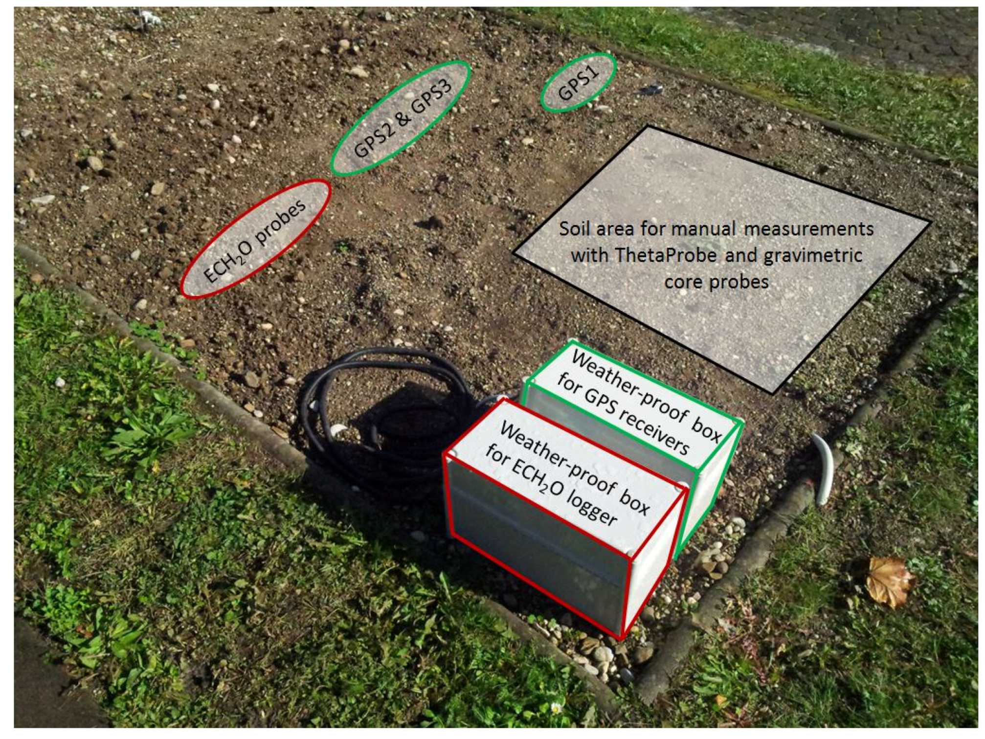
2.1. GPS Measurement Setup at the DWD Test Site Munich

The test site for the GPS SM measurements is situated at the meteorological observation site of the German Weather Service (DWD) in the city of Munich (48°16′43″ N, 11°32′37″ E, 518 m a.s.l.) in Southern Germany. It is well equipped with all standard meteorological measurement instruments. The DWD test site is characterized by a temperate and humid climate of Central Europe with monthly average temperatures ranging from −2 °C in winter to 17 °C in summer. The mean annual precipitation in Munich reaches 930 mm with a summer precipitation peak [41]. Snow cover typically lasts for several weeks in winter, but with a decreasing trend in coverage duration and amount due to climate change [42,43].

The soil of the DWD soil measurement field was classified according to a laboratory soil texture analysis as sandy loam. The average sand and clay content at 10 cm depth are 49% and 7%, respectively. The bulk soil density ${\rho }_b$ is 1.3 g·cm⁻³. As the test site is situated in the Munich gravel plain north of the Northern Calcareous Alps, limestone is the dominant rock type leading to chromic luvisols. The groundwater table in this region is lower than 2.5 m below the surface and due to the low clay content, capillary rise plays a negligible role.

The DWD test site Munich is suitable for soil measurements by GPS. Within a radius of approximately 20 m, the test site is free from surrounding obstacles like houses or trees and allows relatively undisturbed GPS measurements for a city location. We installed three low-cost GPS sensors at the vegetation-free DWD soil measurement field (see Figure 1). One sensor (GPS1) was mounted directly on top of the soil and the other two sensors (GPS2 and GPS3) were installed at a depth of 10 cm within the soil column and were displaced horizontally to avoid being obstructed by the top one. The reason why we installed two GPS sensors in the soil is for redundancy purposes because maintenance of buried sensors is difficult under running conditions and to verify their high correlation, as stated in Section 3.2.

The measurement period was from 1 January 2014 to 10 June 2015. Apart from a system failure for approximately four days at the beginning of the measurement period (25–29 January 2014) and another two days close to the end of the measurement period (27–29 April 2015) due to power failure and a delayed reset, the GPS sensors operated without interruption in a continuous mode. However, days with snow cover and frozen soil were excluded from the analysis in this paper, as snow on top of the soil, especially when it turns wet [37], and also soil frost, have a clear influence on the received GPS signal strength and can therefore influence the exact GPS SM retrieval. To avoid creeping temperature effects within the cables, a temperature threshold of 2 °C was chosen for the air as well as the soil temperature at a depth of 5 cm. In winter 2013/14, only very few days were affected by snow or soil frost; however, in winter 2014/15, there were longer snow periods where we excluded the entire winter months of December 2014 as well as January and February 2015 from this analysis.

Regarding the technical equipment, we used Fastrax IT 430 GPS receivers [44] with integrated SiRF IV chips and stored them together with a temperature-robust and fan-less outdoor PC in a weather-proof box (see Figure 1). The receivers were connected via 3-m coax cables with small (3.9 cm × 3.9 cm) Hirschmann GPS7M magnetic mount antennas [45]. The raw data were stored on the PC, which was driven by electric power provided by the test site. The GPS system was controlled and driven by receiver-specific GPS software. As we used low-cost GPS components, which are easily available and utilized for numerous technical applications like smartphones, cameras or car navigation, the hardware costs of one antenna and receiver pair are quite low, approximately 150 USD, excluding weather-proof boxes, data storage and power supply. Taking all components into account, the applied hardware might be in a similar price range as standard FD or TDR probes.

2.2. Accompanying in Situ Data

Besides the GPS sensors, we installed three ECH₂O EC-5 and two ECH₂O TM frequency domain (FD) probes (Decagon Devices, Pullman, WA, USA) to continuously measure SM at soil depths of 5 cm (three probes) and 10 cm (two probes). In the following, both sensor types will be named ECH₂O probes. The measurement devices are located approximately 0.5 m apart from the buried GPS antennas within the same soil measurement field (see Figure 1). All ECH₂O probes were installed horizontally with the prongs pointing in a horizontal direction. As suggested in Bogena, et al. [46], we applied a sensor-specific correction procedure based on ECH₂O temperature readings to adjust the SM values for each time step. Due to battery failures, two data interruptions of the ECH₂O sensors of a few days occurred (18–21 October 2014 and 1–3 March 2015). During field campaigns, which were conducted in a weekly to bi-weekly rhythm, we regularly measured surface SM with ThetaProbe ML2x FD probes (Delta-T Devices, U.K.) as well as standard manual gravimetric core probes. Further, we used hourly meteorological DWD data encompassing precipitation, air temperature and soil temperature at a depth of 5 cm as well as daily snow height data.

2.3. Land-Surface Model PROMET

The hydrologic land-surface PROcesses of Mass and Energy Transfer (PROMET) model is physically based and describes all relevant water and energy fluxes [8,39,47]. We modelled at a point scale and in an hourly resolution all relevant hydrological parameters for the DWD test site Munich. PROMET was driven by meteorological input data measured at the station and provided by the DWD. The output data, especially the SM, have successfully been validated within different studies, locations and at different scales (e.g., [14,39,48,49,50]). The soil water dynamics in PROMET are simulated with a four-layer soil model applying an explicit solution of the Richards equation for flow in unsaturated media [51]. The soil water retention model of Brooks and Corey [52] is used to relate soil suction head to SM content; a detailed description is given in Mauser and Bach [39] and Muerth and Mauser [53]. Muerth [54] evaluated the soil temperature modelling abilities of PROMET in the Upper Danube Catchment with measurements and remote-sensing data. According to Schlenz et al. [55], modelled and measured SM data were compared extensively on different scales and locations in several large scale field campaigns around Munich between 2007 and 2012 and a detailed analysis of the SM modelling abilities and uncertainties of PROMET is given. The soil water model has been validated with good results, e.g., by Loew et al. [14] and Schlenz et al. [55]. The model results were inter alia used to validate passive microwave remote sensing recordings from the SMOS mission [28,56,57].

For this study, the soil layers were selected to be situated at 0–5, 5–10, 10–45 and 45–145 cm depths. PROMET reports on the vertical average of each selected soil layer. The soil model parameterisation was done according to the soil texture analysis in the laboratory. For all comparisons between modelled and measured SM, the first two PROMET soil layers were used, as these correspond to the 10 cm surface soil layer that is considered with the GPS measurements. From the model output, we used SM, percolation and evaporation information.

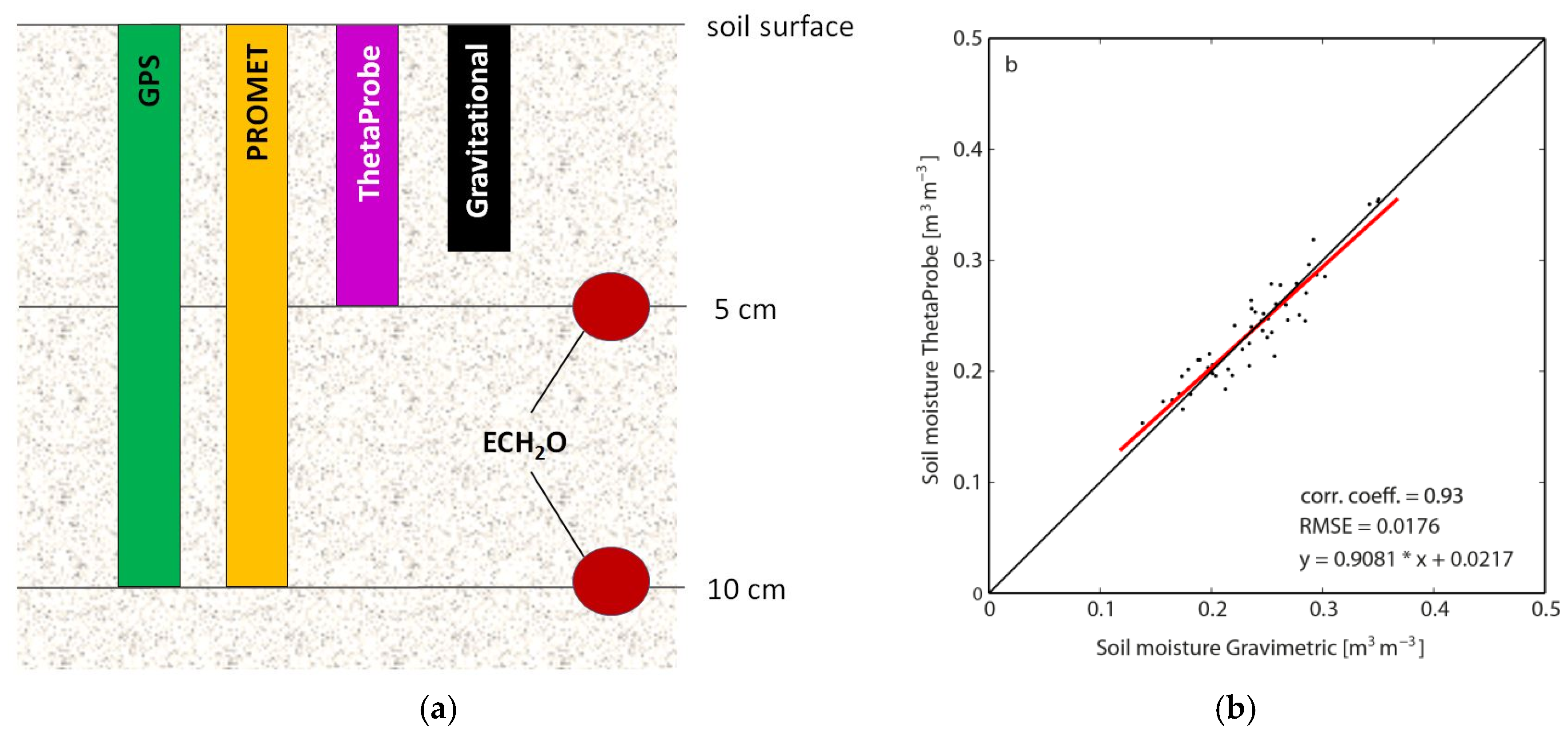
2.4. Soil Moisture Sampling Volumes and Vertical Ranges of Different Methods

Currently, several in situ SM measurement methods exist at an operational level. However, they may differ in their results as they use different techniques, are based on different sampling volumes, may disturb the original soil column or are affected by air or fluid gaps around their prongs [58]. Moreover, the results might be site specific and the sensor sensitivity might vary with the SM content [59].

In this study, we applied the four different measurement methods ECH₂O, ThetaProbe, gravimetric measurement and GPS as well as the model PROMET to derive SM at the DWD test site in Munich. As they are all based on different techniques, vary in sample volume or cover different soil layers, their comparability is restricted. Figure 2a gives an overview on the vertical location and measurement range in the soil column with a depth of 10 cm.

The ECH₂O EC-5 and ECH₂O TM probes reach an estimated sampling volume of 10.5 cm³ and of 15 cm³, respectively [60]. As these sensors have a small sampling volume, they can only give valid information about the SM conditions in their direct vicinity, in this case at approximately 5 and 10 cm soil depth as illustrated in the schematic in Figure 2a. The readings of the five ECH₂O sensors showed high conformity. The correlation of the sensors at a depth of 5 and 10 cm was high with a correlation coefficient of 0.96 and root mean square error (RMSE) of 0.0115 m⁻³·m⁻³. In the following, the mean of all ECH₂O measurements was taken.

The prongs of the FD sensor ThetaProbe are 5 cm in length and they cover an approximate sampling volume of 50 cm³, whereas the gravimetric measurements cover a standardized soil volume of 100 cm³ with a sampling depth of 4 cm. Regarding the measurement depth and vertical location at the top of the soil column, ThetaProbe and the gravimetric measurements are the most similar. Therefore, we used the gravimetric measurements mainly to validate the ThetaProbe readings. As illustrated in Figure 2b, these two methods show high correlation with a correlation coefficient of 0.93 and a RMSE of 0.0176 m⁻³·m⁻³. Therefore, further calibration of the ThetaProbe was not necessary.

The GPS technique encompasses a bulk soil column of 10 cm and is not directly comparable to the other three conventional measurement techniques. Due to the hemispherical GPS satellite coverage, the sensors capture on average a circular cone above the buried antennas. The volume of the circular cone above each antenna is variable as it depends on the SM content. Due to more pronounced refraction processes in wet soils, the path length for electromagnetic waves, especially those with oblique angles, is shortened [11]. This may lead to a significant sampling volume reduction compared to dry soils. The volume with a GPS antenna installation depth of 10 cm and a cut-off elevation angle of 10 degrees encompasses approximately 665 cm³ for absolutely dry soils and approximately 50 cm³ for very wet soils, exemplarily calculated for a quite high SM content of 40 m³·m⁻³ regarding the observed soil in this study.

The main advantage of the model PROMET is that it can calculate the SM of entire soil layers, which makes it more comparable to the GPS bulk measurements over an entire soil layer than, e.g., single ECH₂O SM measurements at specific soil depths. For this study, we used the SM modelled by PROMET from the first two layers, accounting for a soil depth of 10 cm, which is comparable to a vertical integral soil column considered by the GPS measurements.

3. Soil Moisture Retrieval with GPS

3.1. GPS Data Processing

The GPS data processing to retrieve SM is quite analogous to the GPS data processing to retrieve liquid water content in snow, which was described in Koch et al. [37]. In this section, we emphasise the main steps; for more details consider Koch et al. [37]. With the Fastrax IT 430 receivers, we tracked the GPS raw data of the freely available L1 C/A code at a temporal resolution of 1 s, which is broadcasd at a frequency of 1.57542 GHz. The GPS system encompasses in total 32 GPS satellites grouped in six orbits with an equatorial inclination of 55 degrees. Each satellite is seen by the DWD test site in Munich for several hours during a sidereal day (~23 h 56 min). For each time step, the hemispherical satellite coverage ranges between eight to twelve satellites. As all three GPS sensors are situated very close together, the pattern of the satellite trajectories for each sidereal day can be assumed identical.

The carrier-to-noise power density ratio (C/N₀) is included in the GPS raw data and gives information on the received signal strength of each tracked satellite [61]. In a first step, we extracted the C/N₀ received from each GPS satellite at a certain elevation and azimuth angle from the raw data for each time step. Signals below a satellite elevation of 10 degrees were masked out due to too weak signal strength and possible influences from the surrounding. As the received signal strength can vary at different azimuth and elevation angles, we defined 16 azimuth and 16 elevation classes for each of the 32 satellites according to Koch et al. [37]. The reasons for this procedure are that the gain of the low-cost antennas is angle-dependant, the signal strength might vary slightly for each satellite; furthermore, multipath patterns might occur. In a second step, we defined a sidereal reference day during dry and stable soil and atmospheric conditions. For this study, the UTC time period 13:26 16 June 2014–13:22 17 June 2014 was chosen. This period was characterized by stable and low SM conditions due to no rainfall, percolation, capillary rise and negligible condensation over the last seven days. We assume that during this reference period, the recorded C/N₀ values theoretically present the same signal strength [37]; however, the recorded absolute values differ for different elevation and azimuth angles as described above. The measurement at GPS1, which is located above the soil column, corresponds to $I_{m1}$ for each class (see Figure 3). To take the different azimuth and elevation patterns of each antenna into account, we scaled the reference data of GPS1 to the antenna characteristics of GPS2 and GPS3, respectively. In a last step, the measurements recorded within the soil column at GPS2 and GPS3 for each class and each time step, which correspond to $I_{m2,3}$, were set into relation to $I_{m1}$ to calculate the signal attenuation as described in the next section. For the SM calculations, slight temporal fluctuations due to different atmospheric conditions have no decisive impact and can be neglected according to Schmid et al. [38] as described for the retrieval of snow liquid water content.

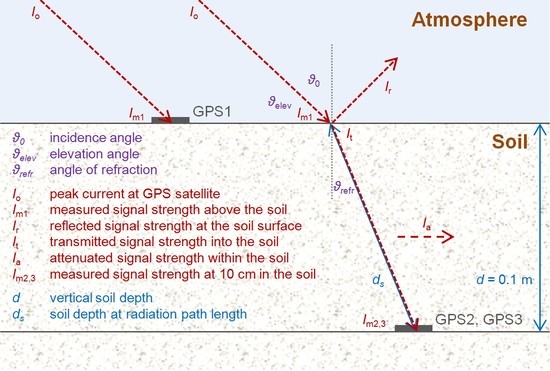
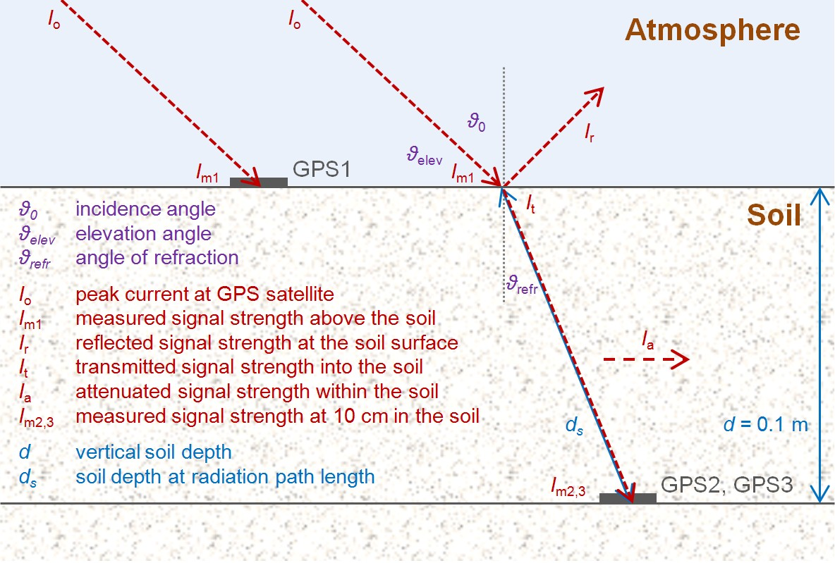
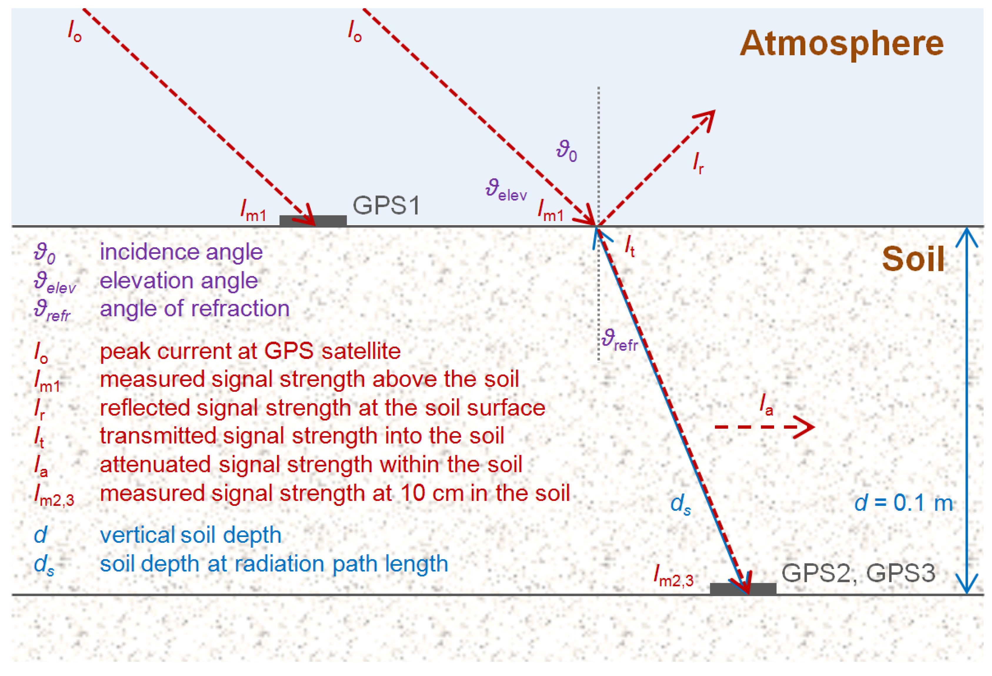
3.2. GPS Signal Strength Attenuation

The calculation of the SM is based on signal strength changes according to dielectric soil properties in connection with electromagnetic waves. We considered reflection, refraction and attenuation processes quite analogous to Koch et al. [37]. Instead of the input value snow depth, we used the installation depth of GPS2 and GPS3 at a soil depth of 10 cm. For this approach, we calculated the reflection and refraction for each single elevation value as already reported in Schmid et al. [38], whereas in Koch et al. [37], only the mean elevation angle was considered. The Equations (1)–(12) in Koch et al. [37] were analogously applied for this study. However, instead of considering the complex permittivity of snow, for this approach, we considered the complex permittivity of soil, which is described in Section 3.3. The measured intensity $I_{m2,3}$ within the soil column as the mean of GPS2 and GPS3 at a soil depth $d_s$ = 0.1 m is described by

$$I_{m2,3}=I_t-I_a=I_{m1}-I_r-I_a$$

(1)

where $I_{m1}$ is the received intensity at GPS1 above the soil, $I_t$ the transmitted intensity into the soil, $I_a$ is the intensity loss due to signal attenuation within the soil, and $I_r$ is the reflected intensity at the interface of air and soil. Figure 3 gives a schematic overview. The calculation of the reflection and refraction is analogous to Koch et al. [37]. As the main outcome, the attenuation coefficient $\alpha$ is calculated by applying Beer-Lambert’s law:

$$\alpha =-\frac{\text{ln}(\frac{I_t-I_a}{I_t})}{d_s}= - \frac{\text{ln}(\frac{I_{m2,3}}{I_{m1}-I_r})}{d_s}$$

(2)

The results for $\alpha$ from GPS2 and GPS3 achieved high agreement with a correlation coefficient of 0.94 and an RMSE of 0.0165 m⁻³·m⁻³, which implies a high reliability of the two GPS sensors below the soil. However, slight differences might occur due to different soil textures above the single antennas. For the further data processing, the average of both antennas within the bulk soil column was taken. Multiple reflections above the soil, e.g., at small obstacles or surrounding vegetation, or within the observed soil column might occur. However, these effects are difficult or even impossible to address, and we assume that they are minor compared to the considered reflection, refraction and attenuation processes, especially considering such a flat site.

3.3. Dobson Four-Component Dielectric Mixing Model

With dielectric models, the SM can be calculated for a specific soil based on its dielectric characteristics within a specific microwave domain. For this study we applied the Dobson four-component dielectric mixing model [40], which is based on the real ${\epsilon }^{\prime }$ and imaginary part ${\epsilon }^{″}$ of the complex permittivity ($\epsilon ={\epsilon }^{\prime }+ i {\epsilon }^{″}$). It describes the behaviour of moist soils at frequencies between 1.4 and 18 GHz, which encompass the GPS L1-band frequency at $f$ = 1.57542 GHz. Besides the four-component mixing model, a semi-empirical soil moisture mixing model is described in Dobson, et al. [40]. However, its performance for lower frequencies around 1.4 GHz is worse than the four-component dielectric mixing model [40]. It was therefore not applied in this study.

Wet soils consist of solid soil particles, air pockets and liquid water. The latter can be further divided into bound water, in a so-called Stern layer, and into bound water in a so-called Gouy layer; the former contains the first few molecular layers surrounding the soil particles; the latter is able to move in the soil medium [40]. Thereafter, the Dobson soil moisture model considers relative permittivities of the four components dry solids ${\epsilon }_{ds}$, bound water ${\epsilon }_{bw}$, bulk water ${\epsilon }_{fw}$ and air ${\epsilon }_a$. The wet soil permittivity ${\epsilon }_{ws}$ is defined as

$${\epsilon }_{ws}=\frac{3{\epsilon }_{ds}+2V_{fw}({\epsilon }_{fw}-{\epsilon }_{ds})+2V_{bw}({\epsilon }_{bw}-{\epsilon }_{ds})+2V_a({\epsilon }_a-{\epsilon }_{ds})}{3+V_{fw}\left(\frac{{\epsilon }_{ds}}{{\epsilon }_{fw}}-1\right)+V_{bw}\left(\frac{{\epsilon }_{ds}}{{\epsilon }_{bw}}-1\right)+V_a\left(\frac{{\epsilon }_{ds}}{{\epsilon }_a}-1\right)}$$

(3)

with $V_{fw}$, $V_{bw}$ and $V_a$ as the volume fractions of free water, bound water and air, which are dependent on the water content in the pores [40]. The entire bulk soil moisture $m_v$ is given by

$$m_v=V_{fw}+V_{bw}$$

(4)

where $V_{bw}$ makes up only a small part. It was calculated after Dobson et al. [40] and was set to 0.191 for the soil observed in this study. The real part of the complex permittivity of dry soil ${\epsilon }_{ds}^{\prime }$ is

$${\epsilon }_{ds}^{\prime }={(1.01+0.44{\rho }_s)}^2-0.062$$

(5)

with ${\rho }_s$ = 2.65 g·cm⁻³ as the mean specific density of the soil paste [11] whereas the measured bulk soil density ${\rho }_b$ = 1.3 g·cm⁻³. The imaginary part of dry soil is negligible. Values for ${\epsilon }_a$, ${\epsilon }_{ds}$ and ${\epsilon }_{bw}$ are given in

Table 1. Values for the real and imaginary part of the complex permittivity of air ${\epsilon }_a$, dry soil ${\epsilon }_{ds}$ according to the soil properties of the observed soil and bound water ${\epsilon }_{bw}$ [40].

Permittivity of Medium	Real Part ε′	Imaginary Part ε″
${\epsilon }_a$	1.00	0.00
${\epsilon }_{ds}$	2.44	~0.00
${\epsilon }_{bw}$	35.00	15.00

.

At a given frequency $f$, the complex permittivity of free bulk water ${\epsilon }_{fw}$ is assumed as a modified Debey-type relaxation [62,63] and is due to the relaxation time of pure water ${\tau }_w$ and the static dielectric constant of water ${\epsilon }_{w0}$ dependent on the soil temperature. As the permittivity of wet soil is slightly temperature dependent, we took soil temperature data measured by the DWD into account. The real part is defined as

$${\epsilon }_{fw}^{\prime }={\epsilon }_{w\infty }+\frac{{\epsilon }_{w0}- {\epsilon }_{w\infty }}{1+{(2\pi f{\tau }_w)}^2}$$

(6)

with ${\epsilon }_{w\infty }$ = 4.9 as the high frequency limit of the permittivity of water. For more information on the calculation of ${\epsilon }_{w0}$, ${\epsilon }_{w\infty }$ and ${\tau }_w$, consider Ulaby et al. [11] and Lane et al. [63]. The imaginary part of the complex permittivity of free bound water is defined as

$${\epsilon }_{fw}^{″}=\frac{2\pi f{\tau }_w({\epsilon }_{w0}- {\epsilon }_{w\infty })}{1+{(2\pi f{\tau }_w)}^2}+ \frac{0.1{\sigma }_{m_v}}{2\pi {\epsilon }_{0}f}$$

(7)

where ${\epsilon }_0=8.854 \times {10}^{-12}$ is the permittivity of free space. It takes the effective conductivity of water ${\sigma }_{m_v}$ [40,63] into account, which is calculated by

$${\sigma }_{m_v}=({\sigma }_G+{\sigma }_{\mathrm{s}})\left(\frac{1-\frac{{\rho }_b}{{\rho }_s}-{\rho }_b{A}_s{d}_{\delta }\times {10}^{-4}}{m_v}\right)$$

(8)

where ${\sigma }_G$ = 2.723 mS·cm⁻¹ is the average conductivity in the Gouy layer, ${\sigma }_{\mathrm{s}}$ = 0.792 mS·cm⁻¹ the conductivity of the soil paste, $A_s$ = 49 m²·g⁻¹ the specific particle surface, which correlates with the clay content, and $d_{\delta }$ = 3 Å. These soil-specific values were derived by or were taken from literature [40] describing a very similar soil type with a low clay content of 8%.

Table 2. Values for the real and imaginary part of the complex permittivity of free bulk water ${\epsilon }_{fw}$ at different Soil temperature.

Soil Temperature	Real Part ε′	Imaginary Part ε″
0.1 °C	85.57	23.81
10 °C	82.76	19.42
20 °C	79.47	16.55
30 °C	76.12	14.75
40 °C	72.95	13.61

shows changes in the real and imaginary part of the complex permittivity of the free bulk water ${\mathsf{\epsilon }}_{\text{fw}}$ due to different soil temperatures.

3.4. Calculation of Soil Moisture and Sensitivity

The attenuation coefficient $\alpha$ was described by Equation (2) in Section 3.2, based on GPS measurements. Moreover, the attenuation coefficient $\alpha$ of a medium like a wet soil can also be calculated in theory by the complex permittivity of wet soil with an emphasis on the imaginary part as:

$$\alpha =\sqrt{\frac{{\mu }_0}{{\epsilon }_{ws}^{\prime }{\epsilon }_0}}{\epsilon }_{ws}^{″}{\epsilon }_{0}2\pi f$$

(9)

where ${\epsilon }_{ws}^{\prime }$ and ${\epsilon }_{ws}^{″}$ are calculated after Equation (3) considering the real and imaginary part. With a root-finding algorithm, we were able to set Equations (2) and (9) equal and could determine, as the only unknown of this approach, the soil moisture $m_v$ under consideration of all soil specific reflection, refraction and attenuation processes for each time step. Potential temperature effects on the GPS sensors causing potential signal strength changes were not taken into account for this approach.

In general, the retrieval of SM with GPS depends on several physical soil parameters, which should be correctly investigated and determined to achieve precise results. However, to get an impression of how sensitive they are, we carried out a sensitivity analysis regarding the parameters soil density, soil texture and soil temperature. This aspect is described and discussed in Section 5.3.

4. Results

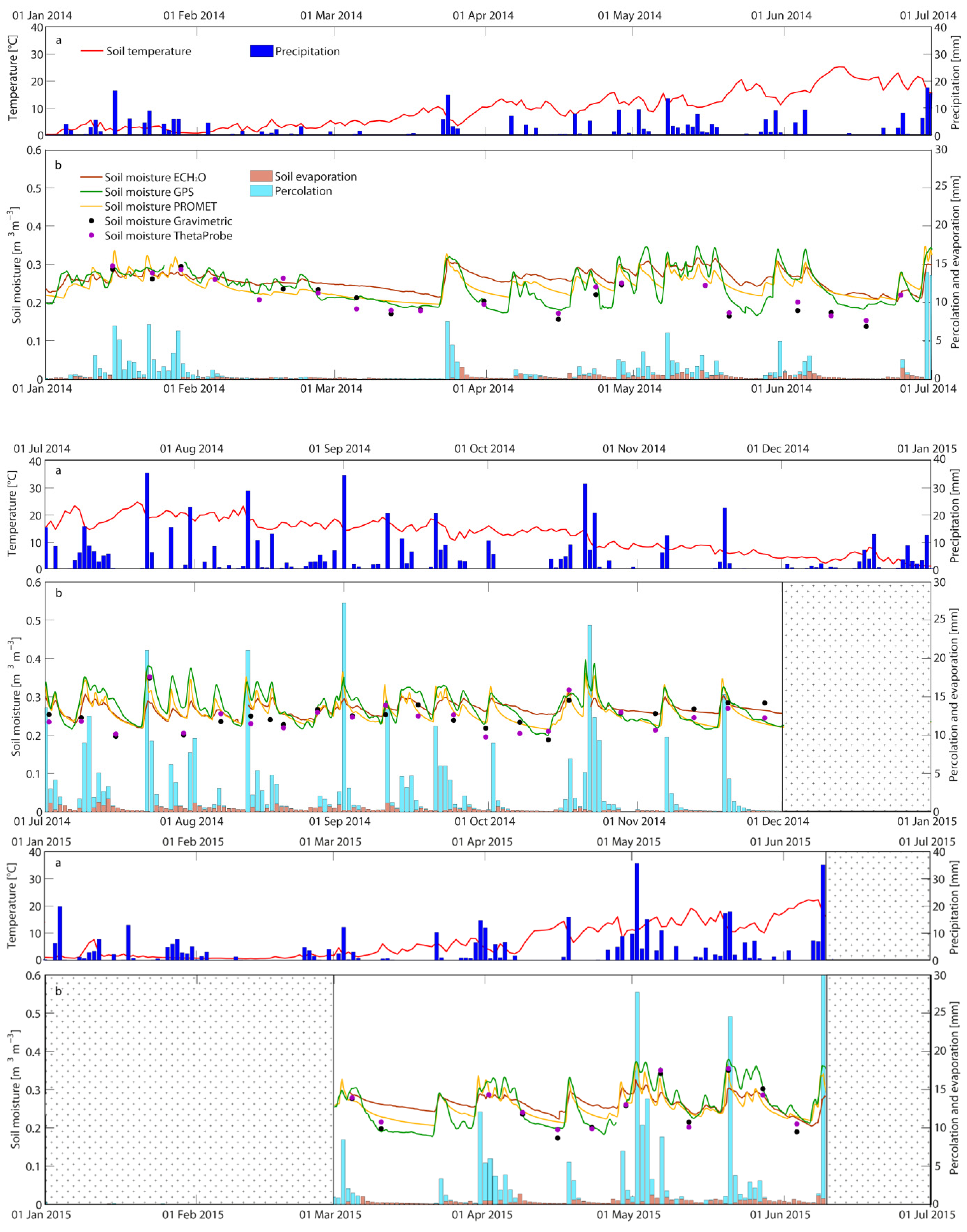
4.1. Time Series of Soil Moisture and Hydrological Data

During a period of almost 1.5 years (1 January 2014–10 June 2015), the SM of the upper ten centimetres at the soil measurement field at the DWD test site in Munich was retrieved from GPS attenuation measurements and other methods (Figure 2a). Figure 4a gives an overview on the soil temperature at a soil depth of 5 cm and precipitation evolution in daily resolution, which was directly measured at the DWD test site in Munich for the entire period. Figure 4b illustrates the evolution of the SM derived by GPS, measured by the Decagon FD ECH₂O probes and modelled by PROMET in daily resolution. Moreover, the weekly to bi-weekly manual measurements with the Delta-T FD ThetaProbe and the gravimetric probe are shown.

As described in Section 2.1, the entire winter months of December 2014 and January and February 2015 were excluded due to potential snow cover or soil frost. Moreover, percolation and soil evaporation modelled with PROMET are presented. Water infiltration into the soil and percolation are largely coupled with precipitation events. However, the daily percolation sums are lower than the daily precipitation sums as evaporation and direct surface runoff occur as well. On the one side, the evaporation rate depends on the available free water and on the other side, also on suitable temperatures. Regarding the investigated soil during the entire measuring period, capillary rise was negligible and the soil evaporation was low and was only pronounced when the temperatures were above approximately 10 °C, indicating high solar radiation and when free soil water was available in the first soil layer, e.g., after a rainfall event.

In Figure 4a,b, regarding all methods, a direct relationship between SM increase and occurrence of percolation is obvious after precipitation events, when water infiltrated into the soil. This is especially the case after 1 July 2014. However, comparing the three continuous methods, the increase in SM of the ECH₂O probes is slightly lower, whereas for GPS more pronounced, PROMET is again in between. During periods with no or low percolation, SM declines slowly. Again, the GPS SM shows the clearest decline, followed by PROMET and then by the ECH₂O probes. The first six months of the measurement period (January–June 2014) were rather dry with only few light rainfall events. Consequently, as the temperatures started to rise in March 2014, SM declined especially in the upper four to five centimetres as the manual ThetaProbe and gravimetric measurements show. Considerable dry periods occurred besides the first six months as well as in November 2014 and March to May 2015.

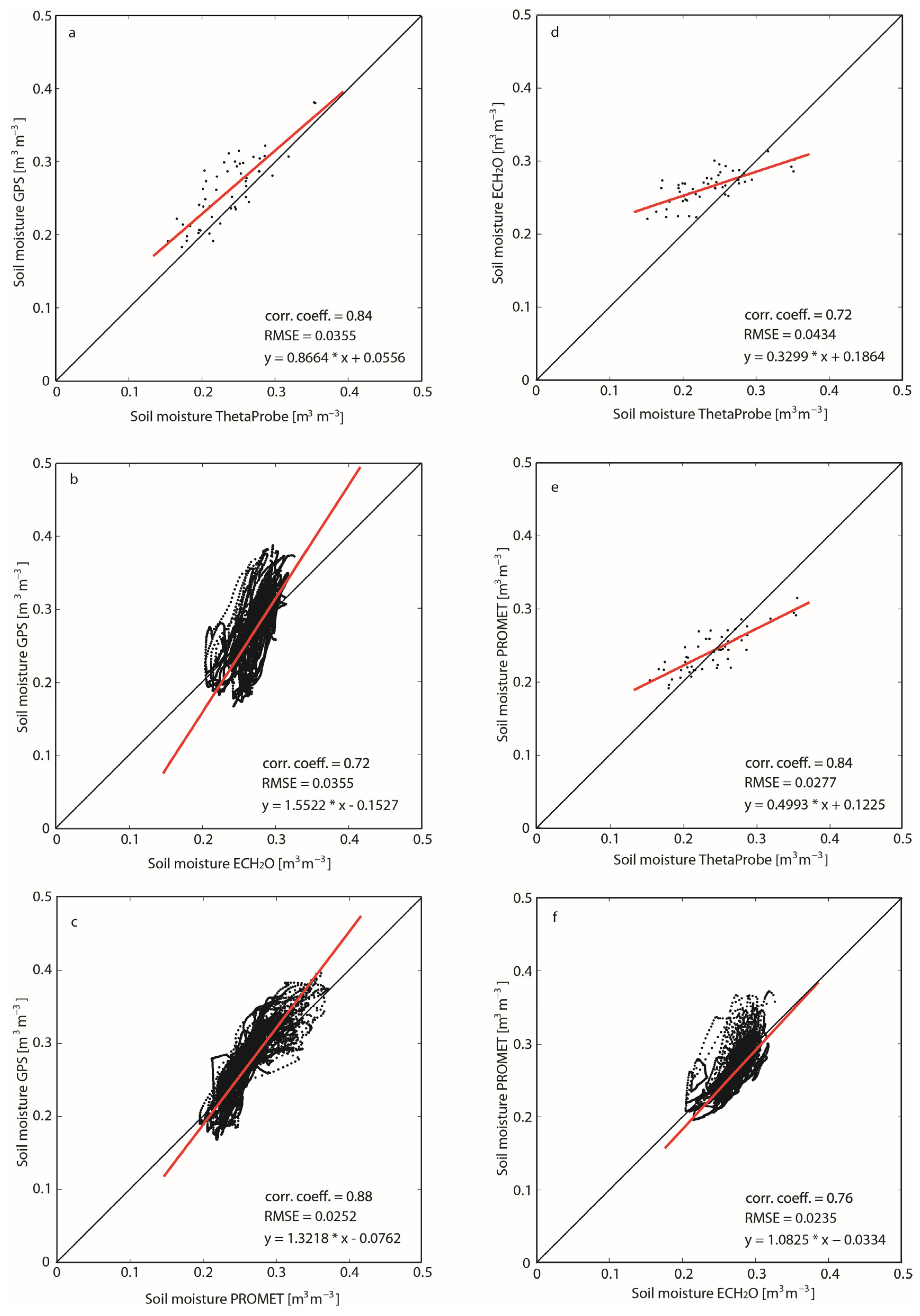
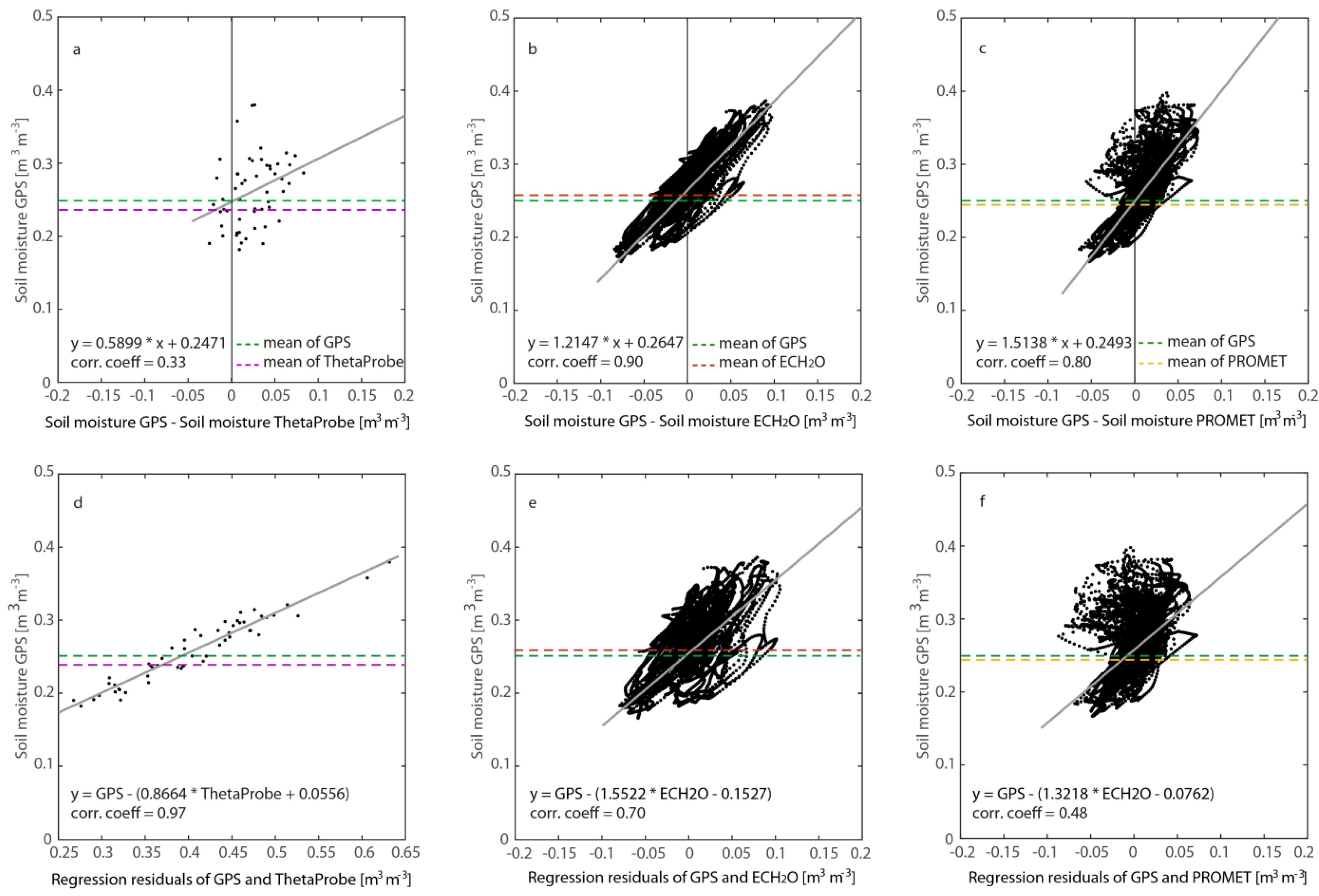
4.2. Comparison of the Different Soil Moisture Methods

During the entire period, the SM curves derived from the continuous measurements with GPS and ECH₂O probes as well as the modelled PROMET data show high conformity. The GPS SM exhibits the highest dynamic, whereas the ECH₂O SM reveals the lowest. PROMET is in between but mostly closer to the GPS SM. A statistical overview of the minimum, maximum, mean and standard deviation is given in

Table 3. Statistical overview of the soil moisture retrieval from GPS, ECH₂O, ThetaProbe and gravimetric samples as well as the modelled soil moisture with PROMET at the DWD test site in Munich during the measurement period 1 January 2014–10 June 2015.

Method	Mean	Std	Min	Max
GPS	0.2565	0.0469	0.1667	0.3977
ECH2O	0.2633	0.0216	0.2044	0.3268
PROMET	0.2522	0.0314	0.1892	0.3675
ThetaProbe	0.2382	0.0465	0.1535	0.3553
Gravimetric	0.2380	0.0482	0.1379	0.3507

for all methods. The mean of the three continuous methods ECH₂O, GPS and PROMET is similar; however, the standard deviation is highest for the GPS values indicating a high dynamic range. The weekly to bi-weekly manual measurements with the ThetaProbe and gravimetric samples are mostly below the continuous methods, especially during dry periods. This is reflected in the lower mean and minimum values compared to the other methods. However, the two manual measurements exhibit a similar dynamic range to the GPS SM as shown in Table 3.

As Figure 2b indicates, the manual surface SM measurements encompassing the gravimetric method and ThetaProbe show high correlation. As all comparisons with the gravimetric method and all other methods would show similar results compared to the ThetaProbe, they are therefore not explicitly shown as scatter plots in the following. The six scatter plots in Figure 5a–f as well as the correlation coefficient and the RMSE in

Table 4. Statistical overview of the correlation coefficient and the RMSE comparing ThetaProbe, ECH₂O, PROMET and GPS. The upper triangular part (regular) represents the correlation coefficient and the lower triangular part (italics) represents the RMSE.

Method	ThetaProbe	ECH2O	PROMET	GPS
ThetaProbe	-	0.72	0.84	0.84
ECH2O	0.0434	-	0.76	0.72
PROMET	0.0277	0.0235	-	0.88
GPS	0.0355	0.0355	0.0252	-

show all variants of comparisons between GPS, ECH₂O, PROMET and ThetaProbe SM.

Comparing GPS, ECH₂O and PROMET, the RMSE is clearly below 0.04 m⁻³·m⁻³, which is considered as a very high agreement and is often the benchmark for SM retrievals from microwave remote sensing products, e.g., for the SMOS mission, and in situ measurements [20]. The same is true for comparisons of GPS and ThetaProbe SM. Only ThetaProbe SM values have a slightly higher RMSE than 0.04 m⁻³·m⁻³ when compared to ECH₂O measurements. Figure 5a shows a high conformity of the GPS measurements with ThetaProbe values; however, the positive offset of the diagonal indicates that the SM measurements undertaken with the ThetaProbe are mostly lower than those derived from the GPS. The difference between GPS and ECH₂O SM in Figure 5b is due to the lower dynamic range of the ECH₂O measurements. This can also be seen in Figure 5d by comparing ThetaProbe with ECH₂O. In Figure 5e, ThetaProbe has also a higher dynamic range compared to PROMET, which is, however, less so than for the comparison of ThetaProbe and ECH₂O in Figure 5d. Figure 5f gives an overview of the comparison of ECH₂O and PROMET. Especially for higher SM values, explicitly above 0.2 m⁻³·m⁻³, PROMET is more dynamic than ECH₂O. GPS and PROMET reach the highest correlation with a correlation coefficient of 0.88 as shown in Figure 5c. The slight deviation is due to the higher dynamic range of the GPS SM measurements.

In Figure 6a–c, the scatterplots between GPS and the differences between GPS and ThetaProbe, GPS and ECH₂O, and GPS and PROMET are shown, which indicate a multiplicative bias between GPS and the other methods. Regarding the lower or higher SM values, the differences between all methods are most pronounced, especially comparing GPS and ECH₂O and lowest between GPS and ThetaProbe. Reaching higher SM values, PROMET shows a similar high dynamic range compared to GPS, which is indicated by the spreading of the points in the upper part of the scatter plot. Figure 6d–f contains scatterplots of the comparison of SM derived by GPS compared with the regression residuals between GPS and the other methods. As the correlation coefficient is lowest between GPS and the regression residuals of GPS and PROMET, indicating a random distribution, those two methods have the lowest systematic effect. Summarized, they show the highest coincidence of SM values.

5. Discussion

5.1. Conformities and Discrepancies between the Different Soil Moisture Methods

We derived SM data at the DWD test site in Munich using two continuous measurement methods; firstly by GPS sensors, which were investigated for the first time and secondly by FD ECH₂O probes. Further, we manually measured surface SM with FD ThetaProbes and gravimetric probes in a weekly to bi-weekly basis. Moreover, we continuously modelled SM by PROMET.

The agreement of all results from the different methods is high, and all data follow the overall course of dry and wet events during the observation period of almost 1.5 years. The increase in SM after the occurrence of precipitation events with infiltration into the soil as well as long dry periods are covered by all methods. However, as described in Section 2.4, the comparability of these methods is limited due to different sampling volumes and different vertical validity ranges within the soil column. According to the results, differences in the SM readings regarding the different methods can be explained by differences in the SM conditions in the upper 10 cm. For a better understanding, the described bulk soil column of 10 cm can be divided into two layers, firstly in approximately the first 5 cm as the direct air and soil interface and secondly in a slightly deeper layer of 5 to 10 cm soil depth.

The gravimetric and ThetaProbe measurements are taken in the uppermost 4 to 5 cm. It is apparent that during dry periods, this layer dries out more than the 5 to 10 cm layer, as the latter is covered by the surrounding soil particles and has no direct exchange with the atmosphere. In the findings, it can be clearly seen that the two manual methods reach the lowest SM values compared to all other methods during these dry periods (see Figure 6 and Table 3). During wet periods they reach a similar maximum than the other methods because the water percolates quite fast from the surface to the 5 to 10 cm layer in the soil column.

The ECH₂O measurements, which were derived in a layer depth of 5 to 10 cm, show less dynamics but the highest mean value of all methods (see Table 3). In this vertical soil range, soil water is stored for a longer time, the SM content is more stable and influences from the atmosphere are less pronounced.

SM simulated by PROMET considers the entire 10 cm layer. The SM evolution over the entire period is highly correlated with the ECH₂O SM readings derived for the 5 to 10 cm soil depth. However, the SM dynamic range of PROMET is higher, which can be explained by the fact that PROMET also covers the highly dynamic surface processes but shows less dynamic than the manual surface measurements derived by ThetaProbe or gravimetric probes, which only consider the upper centimetres of the soil. It is therefore reasonable that the dynamics of PROMET occur between ECH₂O and the manual methods.

PROMET simulations and GPS measurements consider the same vertical range of the uppermost 10 cm and are therefore most suitable for comparison. Positively, the SM curves of GPS and PROMET fit very well, reach the highest correlation coefficient and a very low RMSE and have a similar dynamic range as well as similar minimum, maximum and mean values (see Figure 5 and Figure 6 and Table 3). However, GPS is slightly more dynamic than the modelled data, especially during dry periods. One reason for this might be that the determined soil texture in the laboratory could be slightly different or inhomogeneous compared to the conditions in the soil plot, which would have an influence on the parameterisation of the PROMET model as well as the Dobson four-component model applied for the GPS approach. This in turn has an influence on the SM calculations with both methods. Secondly, as the GPS measurements undergo reflection, refraction and attenuation processes, which are non-linear, especially in case of high SM gradients within the first 10 cm, the GPS calculations might slightly under- or overestimate SM. This is the case if, e.g., the upper 5 cm are drier or wetter, than the lower 5 cm. This might be the reason why during dry periods, GPS is more similar to the ThetaProbe and gravimetric measurements. In summary, we state that the GPS sensors are more sensitive to the dynamics at the soil surface, which is positive in terms of interpreting events directly at the interface of air and soil.

5.2. Advantages and Limitations of GPS Soil Moisture Measurements

This study successfully demonstrates that low-cost GPS sensors are highly capable of quantitatively and continuously retrieving bulk SM of the upper soil layer in a non-destructive manner. A main advantage is that the GPS antennas are installed below the soil column of interest, in this case the upper 10 cm, which means that the soil above the antennas is unaffected by the sensors after the installation. In contrast, gravimetric measurements are accurate but they are highly destructive as for each sample, soil has to be extracted. Regarding FD and TDR probes, their prongs might influence the soil sampling volume during installation. This could cause destruction of the soil structure that could result in an increased pore volume that can fill up with air or water or compacted soil [58], which is not the case when using the GPS measurement system.

Further, soil is a quite heterogeneous medium. Soil texture, pore size distribution, the soil density, and the existence of large air and water pockets or larger heterogeneities like small rocks might vary largely even at small scales. This makes SM measurements quite difficult and explains the effect that sensors installed next to each other might possibly measure different SM values [58]. As the GPS sensors cover the entire soil column above the antennas, which integrate over potential soil inhomogeneities, uncertainties are reduced due to larger sampling volumes. In contrast, most permanently installed FD or TDR sensors only have small sampling volumes at a certain soil depth.

Moreover, we assume the advantage that the GPS sensors are sensitive to the surface SM. Especially the uppermost centimetres of a soil column, at the interface between air and soil, are subject to a high dynamic in SM due to the direct influence of precipitation as well as intense radiation during dry periods. All these processes can be resolved with high sensitivity by the GPS sensor measurements.

It is also considered as an advantage that the GPS signals are broadcasted in the microwave L-band. For SM observations in general, that band is most suitable because the penetration depth of the electromagnetic waves reaches several centimetres even for moist soils. For dry soils, it can even reach several meters [11,64]. As the L-band is widely and successfully used for SM retrievals from microwave measurements, e.g., from SMOS or SMAP, SM data derived by GPS use the same band and rely on a similar physical basis. Therefore, GPS-retrieved SM measurements could have a high potential as ground truth validation data for L-band microwave products. However, passive microwave systems derive SM through emission and the active microwave systems, and GNSS-R use signal reflections, and the GPS approach presented in this study is mainly based on signal strength attenuation.

As this method was only tested on a bare soil field, no quantitative statements about the SM retrieval capabilities of this GPS SM approach can be made for vegetation covered soils. However, we assume that this approach has high potential for soils covered, e.g., by agricultural crop plants like wheat, barley or even maize. In this case, an additional antenna above the vegetation would have to be installed to extract signal strength information from the plant water content, which has to be considered in the calculation in relation to the reduced signal strength at the antennas placed within the soil. Forest stands, however, might be too reductive for the GPS signals to also extract the underlying soils’ SM.

Nevertheless, the vertical range of the soil column that can be investigated is limited, as at some point the GPS signal strength becomes too weak to be tracked continuously. The maximum installation depth might, however, differ for different soil textures and SM contents. For example, for high elevation angles (>70 degrees), the mean C/N₀ values received above the soil at GPS 1, reached approximately 47 dBHz. At a GPS antenna installation depth of 10 cm at GPS2 and GPS3 and for this specific soil texture, we always received strong enough GPS signals without interruption. During quite dry periods, with an SM content of 20 m³·m⁻³, the mean C/N₀ values of the high elevation angles reached approximately 36 dBHz, whereas they declined to approximately 29 dBHz during wet days, exemplarily at an SM content of 35 m³·m⁻³. However, an antenna installation depth below approximately 20 cm for this soil type, especially under wet soil conditions, makes potentially no practical sense, because the GPS signals would be attenuated excessively before reaching the GPS antennas. This could result in a reception of too weak GPS signals, which are then unreliable, or even longer signal interruptions or no signals at all. We tested this during a short experiment with an SM content of 35 m³·m⁻³ at a depth of 20 cm, where the C/N₀ declined to approximately 19 dBHz considering the high elevation angles; during even wetter conditions the signals were, however, not continuous anymore. Applying this approach potentially to vegetation-covered soils at deeper laying root-zones, it could be difficult or even impossible to derive continuous SM information regarding this specific soil type.

A further limitation regarding this measurement approach might be a too constrained hemispherical coverage, e.g., due to tall buildings and trees in the surroundings or extremely steep mountain slopes and deeply cut valleys, which could cover the direct line of sight of too many GPS satellites to the receiver. However, other than GPS positioning algorithms, our approach to measure SM does not depend on a minimum number of four satellites to find a solution. Theoretically, the signal of one single GPS satellite for each time step would be sufficient.

Last but not least, as for every retrieval algorithm, a wrong parameterization might lead to imprecise results. To obtain an impression of its sensitivity, we carried out a sensitivity analysis in the next section.

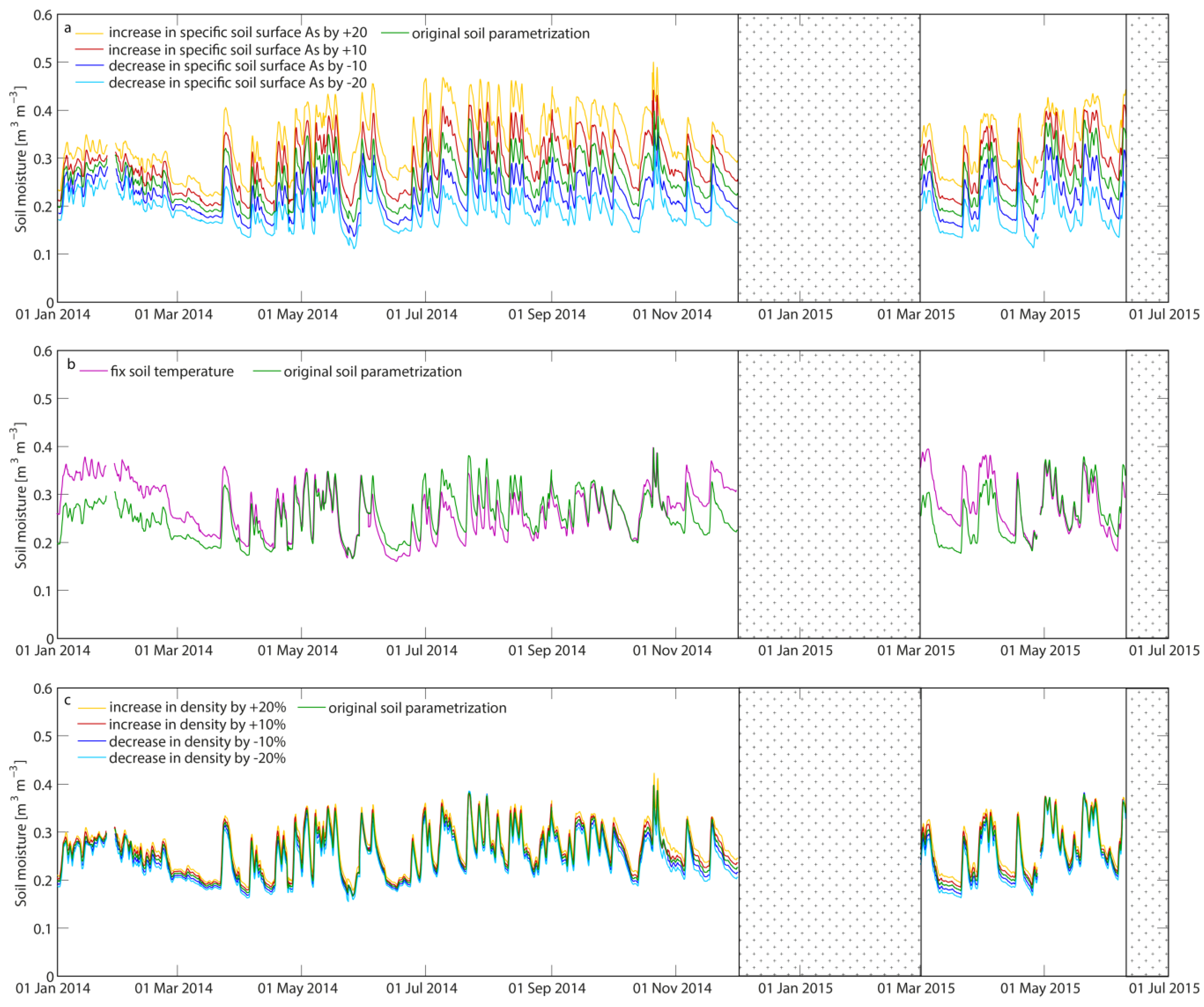
5.3. Sensitivity Analysis of GPS Soil Moisture Measurements

According to Dobson et al. [40] and Hallikainen et al. [65], we investigated the sensitivity of the retrieval algorithm for soil texture and soil temperature, which were identified as the most important physical soil parameters for this approach. In addition, we conducted a sensitivity assessment of the soil density because this parameter exhibited a rather large variability in our soil sampling. For this sensitivity analysis, we applied Equations (1)–(9) analogous to the original and correct soil parameterization.

Regarding different soil textures with different sand, silt and clay contents, the same SM values are based on different values of the complex permittivity of moist soil [40,65]. The soil texture is mainly represented by the physical soil parameter $A_s$, which was set to the value of 49 m²·g⁻¹ for the observed soil at the DWD test site in Munich. Lower values for $A_s$ represent soils with lower clay and higher sand contents, whereas higher values represent higher clay and lower sand contents. We increased and decreased $A_s$ by $\pm 10$ and $\pm 20$. $A_s$ = 29 m²·g⁻¹ represents, for example, the textural class sand and $A_s$ = 69 m²·g⁻¹ silt loam. As shown in Figure 7a, the changes in $A_s$ have quite a large impact on the SM results. If the soil is assumed to be too sandy, SM is underestimated, whereas if it is assumed too clayish, SM is overestimated. In case of an overestimation, the dynamic range increases and in case of an underestimation, it decreases. According to these findings, great effort should be taken to obtain reliable soil texture measurements in the laboratory.

In general, the GPS SM retrieval is based on the complex permittivity of water, which is temperature dependent in the microwave range [40,65] (see also Table 2). For this study, we used separate soil temperature measurements to correctly adapt the Dobson four-component dielectric mixing model. In case no soil temperature readings are available, uncertainties in SM calculations might occur due to wrong soil temperature assumptions. To address this, we additionally calculated for each time step the SM with a fixed soil temperature assumption of 15 °C, which is approximately the average annual soil temperature at the DWD test site. Figure 7b illustrates the difference between the assumed fixed soil temperature and the results with the correct soil temperature. Especially during the colder winter periods, the SM curves deviate the most with a rather high overestimation of up to 8%. However, during warm periods especially in summer, the deviation, expressed as an underestimation, is negligible or less than 2.5%. In case no soil temperature data are available, we recommend an assumption of the soil temperature based on air temperature measurements, if they are available, e.g., from stations nearby. The dynamic range of the air temperature measurements at our test site was only slightly higher than of the soil temperature readings at 5 cm soil depth, which is negligible for the SM results.

To obtain an impression of how soil density variations affect the SM calculations, we decreased and increased the actual measured soil density of ${\rho }_b$ = 1.3 g·cm⁻³ by $\pm 10\%$ leading to densities of 1.17 g·cm⁻³ and 1.43 g·cm⁻³, and $\pm 20\%$ leading to densities of 1.04 g·cm⁻³ and 1.56 g·cm⁻³. Figure 7c shows that these changes in soil density have no severe impact on the SM results. An increase in soil density leads to a slight increase in the SM curve, whereas a decrease in soil density leads to a slight decrease in the SM curve. Though the soil density measurements might not be absolutely accurate, it is still possible to retrieve reasonable SM values.

6. Conclusions

With this new dielectric low-cost GPS approach, we were able to continuously and non-destructively retrieve the bulk soil moisture (SM) of the first 10 cm of bare soil. Our test site was situated at the soil measurement field at the DWD test site in Munich where we installed the sensors for a time period of almost 1.5 years (1 January 2014–10 June 2015). The quantitative retrieval of SM is based on the attenuation of GPS L1-band signals and was calculated with the Dobson four-component soil moisture model based on the complex permittivity.

The temporal evolution of the SM derived by GPS was compared with high conformity to three other measurement methods, namely FD ECH₂O measurements, also in a continuous mode, and weekly to bi-weekly FD ThetaProbe and gravimetric measurements as well as SM simulations with the hydrologic land-surface model PROMET. Comparing all continuous methods, the SM derived by GPS is the most dynamic, showing the greatest minima during dry periods and the highest peaks during intense precipitation. As each method represents the SM values according to different sampling volumes and vertical ranges, their comparability has limitations. However, PROMET and GPS consider the same vertical range and also show the highest conformity. Only during periods with extreme vertical SM gradients, GPS seems to be more dynamic than PROMET. Moreover, all SM curves showed high temporal coincidence with parallel measured precipitation and modelled percolation. In addition, we carried out a sensitivity analysis to address the sensitivity of the applied main physical soil parameters. Overall, an error in the estimation of density is less severe than errors in soil textures and temperature assumptions, especially during cold periods.

In this study, we measured the temporal evolution of SM based on GPS signal attenuation for a bare soil field with a specific soil texture and at a certain soil depth. In a next step, this approach should also be tested for other soil types and different installation depths. Further, this approach could be extended to vegetation-covered soils. For this approach, two antennas above the soil with one situated directly at the soil surface and the second one above the vegetation to extract the signal attenuation of the vegetation layer could be used. Using this extension, near-surface SM could potentially also be derived for vegetation covered soils. This approach would be similar to or could also be combined with the approach of Koch, et al. [37] measuring the liquid water content of snow, with antennas above and below the snow cover. As a technology transfer to hydrological monitoring, the SM and snow cover approaches derived by GPS were already successfully investigated within a thematically specific DFG project and a ESA feasibility study, and are recently under preparation for demonstration as an integrated service within the IAP Demo Project SnowSense (co-funded by ESA under the ARTES 20 program). In general, a major advantage of this approach is that the retrieval of the hydrological observable, which is in this study SM, is based on the microwave L-band. This makes it highly attractive as potential validation data for SM products generated from L-band microwave remote sensing data, like the SMOS or SMAP mission. Moreover, this could complement satellite data with a large spatial coverage but low temporal resolution to extrapolate SM data in a continuous mode at representative sites. As the GPS antennas are installed at a defined soil depth, e.g., 10 cm, the bulk SM of this first soil layer is measured rather than measuring only a small soil volume at a certain depth as is mostly done with FD or TDR sensors. As we use small low-cost and low-power GPS components, the data analysis is not time consuming and the GPS signals can be received globally, and this approach would be suitable to equip entire sensor networks in different regions worldwide. Besides serving as highly useful remote sensing ground truth data and validation data for climate and hydrology studies, SM retrieval based on GPS could also support agricultural studies.

References

1. Dirmeyer, P.A. Using a global soil wetness dataset to improve seasonal climate simulation. J. Clim. 2000, 13, 2900–2922. [Google Scholar] [CrossRef]
2. Kerr, Y.H.; Waldteufel, P.; Wigneron, J.-P.; Delwart, S.; Cabot, F.O.; Boutin, J.; Escorihuela, M.-J.; Font, J.; Reul, N.; Gruhier, C. The SMOS mission: New tool for monitoring key elements ofthe global water cycle. Proc. IEEE 2010, 98, 666–687. [Google Scholar] [CrossRef] [Green Version]
3. Jung, M.; Reichstein, M.; Ciais, P.; Seneviratne, S.I.; Sheffield, J.; Goulden, M.L.; Bonan, G.; Cescatti, A.; Chen, J.; De Jeu, R. Recent decline in the global land evapotranspiration trend due to limited moisture supply. Nature 2010, 467, 951–954. [Google Scholar] [CrossRef] [PubMed]
4. Seneviratne, S.I.; Corti, T.; Davin, E.L.; Hirschi, M.; Jaeger, E.B.; Lehner, I.; Orlowsky, B.; Teuling, A.J. Investigating soil moisture–climate interactions in a changing climate: A review. Earth-Sci. Rev. 2010, 99, 125–161. [Google Scholar] [CrossRef]
5. Koster, R.D.; Dirmeyer, P.A.; Guo, Z.; Bonan, G.; Chan, E.; Cox, P.; Gordon, C.; Kanae, S.; Kowalczyk, E.; Lawrence, D. Regions of strong coupling between soil moisture and precipitation. Science 2004, 305, 1138–1140. [Google Scholar] [CrossRef] [PubMed]
6. Komma, J.; Blöschl, G.; Reszler, C. Soil moisture updating by ensemble Kalman filtering in real-time flood forecasting. J. Hydrol. 2008, 357, 228–242. [Google Scholar] [CrossRef]
7. Loew, A.; Schwank, M.; Schlenz, F. Assimilation of an L-band microwave soil moisture proxy to compensate for uncertainties in precipitation data. IEEE Trans. Geosci. Remote Sens. 2009, 47, 2606–2616. [Google Scholar] [CrossRef]
8. Mauser, W.; Klepper, G.; Zabel, F.; Delzeit, R.; Hank, T.; Putzenlechner, B.; Calzadilla, A. Global biomass production potentials exceed expected future demand without the need for cropland expansion. Nat. Commun. 2015, 6. [Google Scholar] [CrossRef] [PubMed]
9. Fischer, E.; Seneviratne, S.; Lüthi, D.; Schär, C. Contribution of land-atmosphere coupling to recent European summer heat waves. Geophys. Res. Lett. 2007, 34. [Google Scholar] [CrossRef]
10. Loew, A.; Holmes, T.; de Jeu, R. The European heat wave 2003: Early indicators from multisensoral microwave remote sensing? J. Geophys. Res. Atmos. 2009, 114. [Google Scholar] [CrossRef] [Green Version]
11. Ulaby, F.T.; Long, D.G.; Blackwell, W.J.; Elachi, C.; Fung, A.K.; Ruf, C.; Sarabandi, K.; Zebker, H.A.; Van Zyl, J. Microwave Radar and Radiometric Remote Sensing; University of Michigan Press: Ann Arbor, MI, USA, 2014. [Google Scholar]
12. Ulaby, F.T.; Dubois, P.C.; van Zyl, J. Radar mapping of surface soil moisture. J. Hydrol. 1996, 184, 57–84. [Google Scholar] [CrossRef]
13. Dobson, M.C.; Ulaby, F.T. Active microwave soil moisture research. IEEE Trans. Geosci. Remote Sens. 1986, GE-24, 23–36. [Google Scholar] [CrossRef]
14. Loew, A.; Ludwig, R.; Mauser, W. Derivation of surface soil moisture from Envisat Asar wide swath and image mode data in agricultural areas. IEEE Trans. Geosci. Remote Sens. 2006, 44, 889–899. [Google Scholar] [CrossRef]
15. Wagner, W.; Blöschl, G.; Pampaloni, P.; Calvet, J.-C.; Bizzarri, B.; Wigneron, J.-P.; Kerr, Y. Operational readiness of microwave remote sensing of soil moisture for hydrologic applications. Hydrol. Res. 2007, 38, 1–20. [Google Scholar] [CrossRef]
16. Njoku, E.G.; Jackson, T.J.; Lakshmi, V.; Chan, T.K.; Nghiem, S.V. Soil moisture retrieval from AMSR-E. IEEE Trans. Geosci. Remote Sens. 2003, 41, 215–229. [Google Scholar] [CrossRef]
17. Mauser, W.; Rombach, M.; Bach, H.; Demircan, A.; Kellndorfer, J.M. Determination of Spatial and Temporal Soil-Moisture Development Using Multitemporal ERS-1 Data; Satellite Remote Sensing; International Society for Optics and Photonics: Rome, Italy, 1995; pp. 502–515. [Google Scholar]
18. Barré, H.M.; Duesmann, B.; Kerr, Y.H. SMOS: The mission and the system. IEEE Trans. Geosci. Remote Sens. 2008, 46, 587–593. [Google Scholar] [CrossRef]
19. Entekhabi, D.; Njoku, E.G.; Neill, P.E.; Kellogg, K.H.; Crow, W.T.; Edelstein, W.N.; Entin, J.K.; Goodman, S.D.; Jackson, T.J.; Johnson, J. The soil moisture active passive (SMAP) mission. Proc. IEEE 2010, 98, 704–716. [Google Scholar] [CrossRef]
20. Kerr, Y.H.; Waldteufel, P.; Wigneron, J.-P.; Martinuzzi, J.-M.; Font, J.; Berger, M. Soil moisture retrieval from space: The soil moisture and ocean salinity (SMOS) mission. IEEE Trans. Geosci. Remote Sens. 2001, 39, 1729–1735. [Google Scholar] [CrossRef]
21. Katzberg, S.J.; Torres, O.; Grant, M.S.; Masters, D. Utilizing calibrated GPS reflected signals to estimate soil reflectivity and dielectric constant: Results from SMEX02. Remote Sens. Environ. 2006, 100, 17–28. [Google Scholar] [CrossRef]
22. Chew, C.; Small, E.E.; Larson, K.M. An algorithm for soil moisture estimation using GPS-interferometric reflectometry for bare and vegetated soil. GPS Solut. 2016, 20, 525–537. [Google Scholar] [CrossRef]
23. Larson, K.M.; Small, E.E.; Gutmann, E.D.; Bilich, A.L.; Braun, J.J.; Zavorotny, V.U. Use of GPS receivers as a soil moisture network for water cycle studies. Geophys. Res. Lett. 2008, 35. [Google Scholar] [CrossRef]
24. Zavorotny, V.U.; Larson, K.M.; Braun, J.J.; Small, E.E.; Gutmann, E.D.; Bilich, A.L. A physical model for GPS multipath caused by land reflections: Toward bare soil moisture retrievals. IEEE J. Sel. Top. Appl. Earth Obs. Remote Sens. 2010, 3, 100–110. [Google Scholar] [CrossRef]
25. Rodriguez-Alvarez, N.; Bosch-Lluis, X.; Camps, A.; Aguasca, A.; Vall-llossera, M.; Valencia, E.; Ramos-Perez, I.; Park, H. Review of crop growth and soil moisture monitoring from a ground-based instrument implementing the interference pattern GNSS-R technique. Radio Sci. 2011, 46. [Google Scholar] [CrossRef]
26. Rodriguez-Alvarez, N.; Bosch-Lluis, X.; Camps, A.; Vall-Llossera, M.; Valencia, E.; Marchan-Hernandez, J.F.; Ramos-Perez, I. Soil moisture retrieval using GNSS-R techniques: Experimental results over a bare soil field. IEEE Trans. Geosci. Remote Sens. 2009, 47, 3616–3624. [Google Scholar] [CrossRef]
27. Privette, C.V., III; Khalilian, A.; Bridges, W.; Katzberg, S.; Torres, O.; Han, Y.J.; Maja, J.M.; Qiao, X. Relationship of soil moisture and reflected GPS signal strength. Adv. Remote Sens. 2016, 5, 18–27. [Google Scholar] [CrossRef]
28. Dall’Amico, J.T.; Schlenz, F.; Loew, A.; Mauser, W. First results of SMOS soil moisture validation in the Upper Danube catchment. IEEE Trans. Geosci. Remote Sens. 2012, 50, 1507–1516. [Google Scholar] [CrossRef]
29. De Rosnay, P.; Calvet, J.-C.; Kerr, Y.; Wigneron, J.-P.; Lemaître, F.; Escorihuela, M.J.; Sabater, J.M.; Saleh, K.; Barrié, J.; Bouhours, G. SMOSREX: A long term field campaign experiment for soil moisture and land surface processes remote sensing. Remote Sens. Environ. 2006, 102, 377–389. [Google Scholar] [CrossRef]
30. Delwart, S.; Bouzinac, C.; Wursteisen, P.; Berger, M.; Drinkwater, M.; Martin-Neira, M.; Kerr, Y.H. SMOS validation and the cosmos campaigns. IEEE Trans. Geosci. Remote Sens. 2008, 46, 695–704. [Google Scholar] [CrossRef]
31. Bircher, S.; Balling, J.E.; Skou, N.; Kerr, Y.H. Validation of SMOS brightness temperatures during the hobe airborne campaign, Western Denmark. IEEE Trans. Geosci. Remote Sens. 2012, 50, 1468–1482. [Google Scholar] [CrossRef] [Green Version]
32. Panciera, R.; Walker, J.P.; Kalma, J.D.; Kim, E.J.; Hacker, J.M.; Merlin, O.; Berger, M.; Skou, N. The Nafe’05/Cosmos data set: Toward SMOS soil moisture retrieval, downscaling, and assimilation. IEEE Trans. Geosci. Remote Sens. 2008, 46, 736–745. [Google Scholar] [CrossRef] [Green Version]
33. Jackson, T.J.; Bindlish, R.; Cosh, M.; Zhao, T. SMOS soil moisture validation with us in situ networks. In Proceedings of the 2011 IEEE International Geoscience and Remote Sensing Symposium (IGARSS), Vancouver, BC, USA, 24–29 July 2011; pp. 21–23.
34. Rötzer, K.; Montzka, C.; Bogena, H.; Wagner, W.; Kerr, Y.H.; Kidd, R.; Vereecken, H. Catchment scale validation of SMOS and ASCAT soil moisture products using hydrological modeling and temporal stability analysis. J. Hydrol. 2014, 519, 934–946. [Google Scholar] [CrossRef]
35. Dorigo, W.; Wagner, W.; Hohensinn, R.; Hahn, S.; Paulik, C.; Xaver, A.; Gruber, A.; Drusch, M.; Mecklenburg, S.; Oevelen, P.V. The international soil moisture network: A data hosting facility for global in situ soil moisture measurements. Hydrol. Earth Syst. Sci. 2011, 15, 1675–1698. [Google Scholar] [CrossRef]
36. Wigneron, J.-P.; Kerr, Y.; Waldteufel, P.; Saleh, K.; Escorihuela, M.-J.; Richaume, P.; Ferrazzoli, P.; De Rosnay, P.; Gurney, R.; Calvet, J.-C. L-band microwave emission of the biosphere (L-meb) model: Description and calibration against experimental data sets over crop fields. Remote Sens. Environ. 2007, 107, 639–655. [Google Scholar] [CrossRef]
37. Koch, F.; Prasch, M.; Schmid, L.; Schweizer, J.; Mauser, W. Measuring snow liquid water content with low-cost GPS receivers. Sensors 2014, 14, 20975–20999. [Google Scholar] [CrossRef] [PubMed]
38. Schmid, L.; Koch, F.; Heilig, A.; Prasch, M.; Eisen, O.; Mauser, W.; Schweizer, J. A novel sensor combination (upGPR–GPS) to continuously and non-destructively derive snow cover properties. Geophys. Res. Lett. 2015, 42, 3397–3405. [Google Scholar] [CrossRef]
39. Mauser, W.; Bach, H. PROMET–large scale distributed hydrological modelling to study the impact of climate change on the water flows of mountain watersheds. J. Hydrol. 2009, 376, 362–377. [Google Scholar] [CrossRef]
40. Dobson, M.C.; Ulaby, F.T.; Hallikainen, M.T.; El-Rayes, M. Microwave dielectric behavior of wet soil-part II: Dielectric mixing models. IEEE Trans. Geosci. Remote Sens. 1985, GE-23, 35–46. [Google Scholar] [CrossRef]
41. Mauser, W.; Prasch, M. Regional Assessment of Global Change Impacts: The Project GLOWA-Danube; Springer: Berlin, Germany, 2015. [Google Scholar]
42. Weber, M.; Braun, L.; Mauser, W.; Prasch, M. Contribution of rain, snow-and icemelt in the Upper Danube discharge today and in the future. Geogr. Fis. Din. Quat. 2010, 33, 221–230. [Google Scholar]
43. Koch, F.; Prasch, M.; Bach, H.; Mauser, W.; Appel, F.; Weber, M. How will hydroelectric power generation develop under climate change scenarios? A case study in the Upper Danube basin. Energies 2011, 4, 1508–1541. [Google Scholar] [CrossRef] [Green Version]
44. Fastrax IT430 Data Sheet. Available online: https://upverter.com/datasheet/042ba70ed2cd4485a04760b5e6864a3cad0eca96.pdf (accessed on 12 April 2016).
45. Hirschmann Car Communication. GPS Antennas—Powerful and Flexibly Combined. Available online: http://www.hirschmann-car.com/en/products/antenna-systems/gnss-satellite-positioning/gps/ (accessed on 12 April 2016).
46. Bogena, H.; Huisman, J.; Oberdörster, C.; Vereecken, H. Evaluation of a low-cost soil water content sensor for wireless network applications. J. Hydrol. 2007, 344, 32–42. [Google Scholar] [CrossRef]
47. Mauser, W.; Schädlich, S. Modelling the spatial distribution of evapotranspiration on different scales using remote sensing data. J. Hydrol. 1998, 212, 250–267. [Google Scholar] [CrossRef]
48. Strasser, U.; Mauser, W. Modelling the spatial and temporal variations of the water balance for the weser catchment 1965–1994. J. Hydrol. 2001, 254, 199–214. [Google Scholar] [CrossRef]
49. Prasch, M.; Mauser, W.; Weber, M. Quantifying present and future glacier melt-water contribution to runoff in a central Himalayan river basin. Cryosphere 2013, 7, 889–904. [Google Scholar] [CrossRef]
50. Prasch, M.; Marke, T.; Strasser, U.; Mauser, W. Large scale integrated hydrological modelling of the impact of climate change on the water balance with Danubia. Adv. Sci. Res. 2011, 7, 61–70. [Google Scholar] [CrossRef]
51. Philip, J. The theory of infiltration: 1. The infiltration equation and its solution. Soil Sci. 1957, 83, 345–358. [Google Scholar] [CrossRef]
52. Brooks, R.; Corey, A. Hydraulic Properties of Porous Media; Colorado State University: Fort Collins, CO, USA, 1964. [Google Scholar]
53. Muerth, M.; Mauser, W. Rigorous evaluation of a soil heat transfer model for mesoscale climate change impact studies. Environ. Model. Softw. 2012, 35, 149–162. [Google Scholar] [CrossRef]
54. Muerth, M. A Soil Temperature and Energy Balance Model for Integrated Assessment of Global Change Impacts at the Regional Scale, LMU. 2008. Available online: http://edoc.ub.uni-muenchen.de/8810/ (accessed on 15 April 2016).
55. Schlenz, F.; Dall’Amico, J.T.; Loew, A.; Mauser, W. Uncertainty assessment of the smos validation in the Upper Danube catchment. IEEE Trans. Geosci. Remote Sens. 2012, 50, 1517–1529. [Google Scholar] [CrossRef]
56. Schlenz, F.; Mauser, W.; Loew, A. Analysis of smos brightness temperature and vegetation optical depth data with coupled land surface and radiative transfer models in Southern Germany. Hydrol. Earth Syst. Sci. 2012, 16, 3517–3533. [Google Scholar] [CrossRef]
57. Loew, A.; Schlenz, F. A dynamic approach for evaluating coarse scale satellite soil moisture products. Hydrol. Earth Syst. Sci. 2011, 15, 75–90. [Google Scholar] [CrossRef]
58. Walker, J.P.; Willgoose, G.R.; Kalma, J.D. In situ measurement of soil moisture: A comparison of techniques. J. Hydrol. 2004, 293, 85–99. [Google Scholar] [CrossRef]
59. Mittelbach, H.; Casini, F.; Lehner, I.; Teuling, A.J.; Seneviratne, S.I. Soil moisture monitoring for climate research: Evaluation of a low-cost sensor in the framework of the Swiss Soil Moisture EXperiment (SwissSMEX) campaign. J. Geophys. Res. Atmos. 2011, 116. [Google Scholar] [CrossRef]
60. Limsuwat, A.; Sakaki, T.; Illangasekare, T.H. Experimental quantification of bulk sampling volume of ECH2O soil moisture sensors. In Proceedings of the 29th Annual American Geophysical Union Hydrology Days, Collins, CO, USA, 25–27 March 2009.
61. Hofmann-Wellenhof, B.; Lichtenegger, H.; Wasle, E. GPS; Springer: Berlin, Germany, 2008. [Google Scholar]
62. Cole, K.S.; Cole, R.H. Dispersion and absorption in dielectrics I. Alternating current characteristics. J. Chem. Phys. 1941, 9, 341–351. [Google Scholar] [CrossRef]
63. Lane, J.; Saxton, J. Dielectric dispersion in pure polar liquids at very high radio-frequencies. I. Measurements on water, methyl and ethyl alcohols. In Proceedings of the Royal Society of London A: Mathematical, Physical and Engineering Sciences; The Royal Society: London, UK, 1952; pp. 400–408. [Google Scholar]
64. Nolan, M.; Fatland, D.R. Penetration depth as a dinsar observable and proxy for soil moisture. IEEE Trans. Geosci. Remote Sens. 2003, 41, 532–537. [Google Scholar] [CrossRef]
65. Hallikainen, M.T.; Ulaby, F.T.; Dobson, M.C.; El-Rayes, M.A.; Wu, L.-K. Microwave dielectric behavior of wet soil-part 1: Empirical models and experimental observations. IEEE Trans. Geosci. Remote Sens. 1985, GE-23, 25–34. [Google Scholar] [CrossRef]
Figure 1. Soil measurement field at the DWD test site in Munich. The locations of GPS1, GPS2 and GPS3 as well as the locations of the other soil moisture measurements (ECH2O, ThetaProbe and gravimetric core probes) are marked.
Water 08 00276 g001
Figure 2. (a) Vertical location and measurement range in the soil column of the different methods to derive soil moisture; (b) Validation of ThetaProbe soil moisture readings by comparison with gravimetric measurements at the DWD test site in Munich during numerous field campaigns over the measurement period 1 January 2014–10 June 2015.
Water 08 00276 g002
Figure 3. Overview of influences on the measured GPS intensity and radiation path length through the soil column, as well as the angle changes due to reflection, refraction and attenuation processes according to Koch et al. [37]. Only the direct signal paths are shown for one satellite at a specific elevation (in red).
Water 08 00276 g003
Figure 4. (a) Soil temperature at a soil depth of 5 cm and precipitation measured at the DWD test site in Munich as well as (b) soil moisture measured by GPS, ECH2O, ThetaProbe and gravitationally as well as modelled with PROMET at the DWD test site in Munich during the measurement period 1 January 2014–10 June 2015. The winter time with potential snow cover and soil frost is excluded.
Water 08 00276 g004
Figure 5. Comparison of soil moisture values (a) measured by ThetaProbe vs. measured by GPS; (b) measured by ECH2O vs. measured by GPS; (c) modelled with PROMET vs. measured by GPS; (d) measured by ThetaProbe vs. measured by ECH2O; (e) measured by ThetaProbe vs. modelled with PROMET and (f) measured by ECH2O, vs. modelled with PROMET at the DWD test site in Munich during the measurement period 1 January 2014–10 June 2015.
Water 08 00276 g005
Figure 6. Comparison of soil moisture derived by GPS with the difference between (a) GPS and ThetaProbe; (b) GPS and ECH2O; and (c) between GPS and PROMET as well as with the regression residuals between (d) GPS and ThetaProbe; (e) GPS and ECH2O; and (f) between GPS and PROMET. The linear regression equations to calculate the residuals for each method compared to GPS were taken from the information given in Figure 5a–c, respectively.
Water 08 00276 g006
Figure 7. Soil moisture derived from GPS containing different assumptions on (a) an increase or decrease of the specific soil surface A s , which is an indicator for different soil texture assumptions of ± 10 and ± 20 ; (b) a fixed soil temperature assumption of 15 °C and (c) a soil density over- and underestimation of ± 10 % and ± 20 % compared to the original parameterized calculations at the DWD test site in Munich during the measurement period 1 January 2014–10 June 2015.
Water 08 00276 g007