


Introduction
Grasslands are the most widespread habitat in the world and provide crucial goods and services for human population, including animal feeding, climate regulation and carbon cycling (Hooper et al., Reference Hooper, Chapin, Ewel, Hector, Inchausti, Lavorel, Lodge, Loreau, Naeem, Schmid, Setälä, Symstad, Vandermeer and Wardle2005). Extensively managed mountain grasslands in particular, are some of the most species-rich ecosystems (Wilson et al., Reference Wilson, Peet, Dengler and Meelis2012), store about 100 t/ha of soil carbon (Sjögersten et al., Reference Sjögersten, Alewell, Cecillon, Hagedorn, Jandl, Leifeld, Martinsen, Schindlbacher, Sebastia, Van Miegroet, Jandl, Rodeghiero and Olsson2011), and their net ecosystem exchange (NEE, Woodwell and Whittaker Reference Woodwell and Whittaker1968) is mostly dominated by assimilation (Gilmanov et al., Reference Gilmanov, Soussana, Aires, Allard, Ammann, Balzarolo, Barcza, Bernhofer, Campbell, Cernusca, Cescatti, Clifton-Brown, Dirks, Dore, Eugster, Fuhrer, Gimeno, Gruenwald, Haszpra, Hensen, Ibrom, Jacobs, Jones, Lanigan, Laurila, Lohila, Manca, Marcolla, Nagy, Pilegaard, Pinter, Pio, Raschim, Rogiers, Sanz, Stefanim, Sutton, Tuba, Valentini, Williams and Wohlfahrt2007; Soussana et al., Reference Soussana, Allard, Pilegaard, Ambus, Amman, Campbell, Ceschia, Clifton-Brown, Czobel, Domingues, Flechard, Fuhrer, Hensen, Horvath, Jones, Kasper, Martin, Nagy, Neftel, Raschi, Baronti, Rees, Skiba, Stefani, Manca, Sutton, Tuba and Valentini2007; Berninger et al., Reference Berninger, Susiluoto, Gianelle, Bahn, Wohlfahrt, Sutton, Garcia-Pausas, Gimeno, Sanz, Dore, Rogiers, Furger, Balzarolo, Sebastià and Tenhunen2015).
However, there is still a lack of empirical data, mainly from the high elevations and from some regions, including the Mediterranean basin, in which climate change impacts are projected to be very severe (García-Ruiz et al., Reference García-Ruiz, López-Moreno, Vicente-Serrano, Lasanta-Martínez and Beguería2011). In the particular case of the Pyrenees, despite the few corresponding studies (Wohlfahrt et al., Reference Wohlfahrt, Anderson-Dunn, Bahn, Berninger, Campbell, Carrara, Cescatti, Christensen, Dore, Friborg, Furger, Gianelle, Hargreaves, Hari, Haslwanter, Marcolla, Milford, Nagy, Nemitz, Rogiers, Sanz, Siegwolf, Susiluoto, Sutton, Tuba, Ugolini, Valentini, Zorer and Cernusca2008a; Sjögersten et al., Reference Sjögersten, Llurba, Ribas, Yanez-Serrano and Sebastià2012; Berninger et al., Reference Berninger, Susiluoto, Gianelle, Bahn, Wohlfahrt, Sutton, Garcia-Pausas, Gimeno, Sanz, Dore, Rogiers, Furger, Balzarolo, Sebastià and Tenhunen2015), NEE datasets are very limited, and knowing the particularities of these systems may provide some guidelines to adapt and mitigate climate change effects in this region.
Moreover, mountain grasslands are especially vulnerable to climate and land use changes, and mid- to long-term effects on the carbon budget still remain controversial (Wu et al., Reference Wu, Dijkstra, Koch, Peñuelas and Hungate2011), partly due to complex interactions between environmental variables and vegetation. Indeed, although the role of main environmental CO2 exchange drivers, such as photosynthetically active radiation (Wohlfahrt et al., Reference Wohlfahrt, Hammerle, Haslwanter, Bahn, Tappeiner and Cernusca2008b), temperature and soil moisture (Davidson and Janssens, Reference Davidson and Janssens2006; Albergel et al., Reference Albergel, Calvet, Gibelin, Lafont, Roujean, Berne, Traullé and Fritz2010; Yvon-Durocher et al., Reference Yvon-Durocher, Caffrey, Cescatti, Dossena, Giorgio, Gasol, Montoya, Pumpanen, Staehr, Trimmer, Woodward and Allen2012) has been widely assessed, how they interact with phenology and vegetation composition still needs deeper understanding.
Vegetation in mountain grasslands is highly dynamic, changing its structure and composition over time and space (Faurie et al., Reference Faurie, Soussana and Sinoquet1996; Giunta et al., Reference Giunta, Pruneddu and Motzo2009; Mitchell and Bakker, Reference Mitchell and Bakker2016), resulting in a variable patchy configuration of species (Schwinning and Parsons, Reference Schwinning and Parsons1996), and generating differences in biogeochemical cycles and CO2 exchange (Reich et al., Reference Reich, Walters and Ellsworth1997). While it is known that the aboveground living biomass (AGLB) directly takes-up (Wohlfahrt et al., Reference Wohlfahrt, Hammerle, Haslwanter, Bahn, Tappeiner and Cernusca2008b; Nakano and Shinoda, Reference Nakano and Shinoda2014) and releases CO2 (Kardol et al., Reference Kardol, Cregger, Campany and Classen2010; Thakur and Eisenhauer, Reference Thakur and Eisenhauer2015), phenology and vegetation structure may also be determinant for the NEE. Indices of phenological development related to plant productivity, including total green biomass and normalized difference vegetation index (Gao et al., Reference Gao, Zhu, Schwartz, Ganjurjav and Wan2016; Zhou et al., Reference Zhou, Cai, Qin, Lai, Guan, Zhang, Jiang, Du, Yang, Cong and Zheng2016) have already been used to estimate gross primary production (GPP, Filippa et al., Reference Filippa, Cremonese, Galvagno, Migliavacca, Morra di Cella, Petey and Siniscalco2015) and ecosystem respiration (Reco, Ryan and Law Reference Ryan and Law2005).
However, when assessing mountain grasslands there are differences in phenological cycles between elevation belts (Liu et al., Reference Liu, Liu, Liang, Donnelly, Park and Schwartz2014; Leifeld et al., Reference Leifeld, Meyer, Budge, Sebastia, Zimmermann and Fuhrer2015), which may result in more complex vegetation–CO2 exchange interactions than expected. In addition, there are other vegetation fractions, such as standing dead biomass (SDB,dead biomass attached to the plant) and litter (dead plant material, detached from the plant and laying on the soil surface), which are present in considerable amounts in grasslands, and whose specific role as CO2 exchange drivers has been barely considered (Leitner et al., Reference Leitner, Sae-Tun, Kranzinger, Zechmeister-Boltenstern and Zimmermann2016; Gliksman et al., Reference Gliksman, Navon, Dumbur, Haenel and Grünzweig2018).
On the other hand, vegetation composition has also been reported to drive CO2 exchange fluxes (De Deyn et al., Reference De Deyn, Quirk, Yi, Oakley, Ostle and Bardgett2009; Metcalfe et al., Reference Metcalfe, Fisher and Wardle2011; Ribas et al., Reference Ribas, Llurba, Gouriveau, Altimir, Connolly and Sebastià2015). A common approximation to assess this vegetation–CO2 exchange relationship is to separate plant species into plant functional types (PFT) that share a common response to an environmental factor, ‘response traits’, and/or a common effect on ecosystem processes, ‘effect traits’ (Lavorel and Garnier, Reference Lavorel and Garnier2002). In the specific case of grasslands, species are often classified in grasses, non-legume forbs (hereafter ‘forbs’) and legume forbs (hereafter ‘legumes’), classification that is based on nitrogen and light (and therefore CO2) acquisition and use (Tilman, Reference Tilman1997; Symstad, Reference Symstad2000; Díaz et al., Reference Díaz, Lavorel, McIntyre, Falczuk, Casanoves, Milchunas, Skarpek, Ruschk, Sternberg, Noy-Meir, Landsberg, Zhang, Clark and Campbell2007; defined as ‘guilds’ in Sebastià, Reference Sebastià2007). Thus, legumes have the capacity to fix symbiotic nitrogen, while grasses have some advantages when competing for light as they are usually taller than legumes and forbs, and have erect high-density leaves that ensure good light penetration (Craine et al., Reference Craine, Froehle, Tilman, Wedin and Chapin2001). However, there is still some uncertainty about how these PFT can differentially influence CO2 exchange at a plot scale.
Accordingly, in the present study we investigate the interaction between environmental variables and vegetation on CO2 exchange fluxes, and more specifically we aim to: (1) compare the contribution of vegetation phenology and environmental variables in two climatically contrasted mountain grasslands in the Pyrenees, and (2) assess the influence of vegetation composition, in terms of the dominant PFT (forbs, grasses and legumes), on light response and therefore on NEE. For that purpose, we performed a survey of CO2 exchange measurements with a non-steady state chamber, aboveground biomass sampling and environmental variables recording in two extensively managed mountain grasslands in the Pyrenees, located in the montane and subalpine elevation belts, respectively.
Material and methods
Study sites
The study sites were two grazed mountain grasslands in the south-eastern Pyrenees: La Bertolina (BERT), located in Pla de Busa (42°05′N, 1°39′E, 1276 m a. s. l.), and Castellar de n'Hug (CAST) in Plans del Ginebrar (42°18′N, 2°02′E, 1900 m a. s. l.). Both sites were characterized by a Mediterranean climate regime, with spring and autumn precipitations and relatively high summer temperatures (Fig. 1(a)). However, each grassland had its own specific climatic characteristics and phenological particularities, respective to the given elevation belt.

Fig. 1. Climatic and environmental variables of the study sites: Bertolina (BERT) and Castellar (CAST). (a) Mean climatic (1970–2000) monthly air temperature (Ta, solid symbols and line) and monthly precipitation (bars), source: WorldClim (Fick and Hijmans, Reference Fick and Hijmans2017); (b) 2012 meteorological data: Ta (grey line), and soil water content at 5 cm depth (SWC, black line), lines fitted using generalized additive models with integrated smoothness estimation (gam), mgcv package (Wood, Reference Wood2004), source: eddy covariance flux stations; (c) 2012 normalized difference vegetation index (NDVI, black line) and its 0.95 confidence interval (grey band), line fitted using local polynomial regression fitting (loess), source: eddy covariance flux stations. Vertical black dashed lines indicate the beginning and the end of the study period.
BERT was a typical montane grassland, with a mean annual temperature of 9 °C and a mean annual precipitation of 870 mm (Fig. 1(a)). In BERT, vegetation started to grow (Fig. 1(c)) as soon as soil water content (SWC, Fig. 1(b)) increased, and senescence started (Fig. 1(c)) as soon as SWC dropped and summer temperatures became high (Ta ~ 18 °C, Fig. 1(b)). On the other hand, CAST was a subalpine grassland, with a mean annual temperature of 5.1 °C and a mean annual precipitation of 1189 mm (Fig. 1(a)). CAST was more temperature limited, and vegetation did not start to grow (Fig. 1(c)) until temperatures increased up-to ≥ 5 °C, irrespective of the highest spring SWC, which coincided with the snowmelt period and cold temperatures (Ta ⩽ 5 °C). Senescence started later at CAST than at BERT, and progressed more slowly (Fig. 1(c)), despite the low-mid-summer SWC (Fig. 1(b)).
Vegetation composition at BERT was characteristic of a montane meso-xerophytic grassland, and CAST was a mesic subalpine grassland. Both sites were extensively grazed, by cattle at BERT, with an average stocking rate of 0.44 livestock units (LSU)/ha, from May to November; and by cattle and sheep at CAST, with an average stocking rate of 0.74 LSU/ha, from late June to November (according to the corresponding site managers). The montane grassland (BERT) sustained a lower livestock density, although during a longer time period (~3.1 LSU month/ha/year). On the contrary, the subalpine grassland (CAST) was highly productive during the summer and sustained a higher livestock density, but during a shorter time (~4.4 LSUmonth/ha/year). Farmers' expectation of the carrying capacity was ~44% higher at CAST than at BERT. Grazing calendar and stocking rates were provided by the farmers and later confirmed during sampling visits. Soil at BERT was udic calciustept and at CAST was lithic udorthent (FAO, 1998).
Sampling design
Two sampling designs were established to achieve the aims of the current paper: a seasonal and a diel sampling. The aim of the seasonal sampling was to record temporal CO2 variability over the growing season and its relationship with environmental variables and vegetation phenology. The seasonal sampling was carried out from April to December of 2012, at 3-weekly intervals. Every sampling day, sampling points of grassland patches (n = 10 at BERT and n = 8 at CAST) were systematically placed within the footprint of the respective eddy covariance flux stations previously installed at each site (Fig. 2), which provided ancillary meteorological variables.
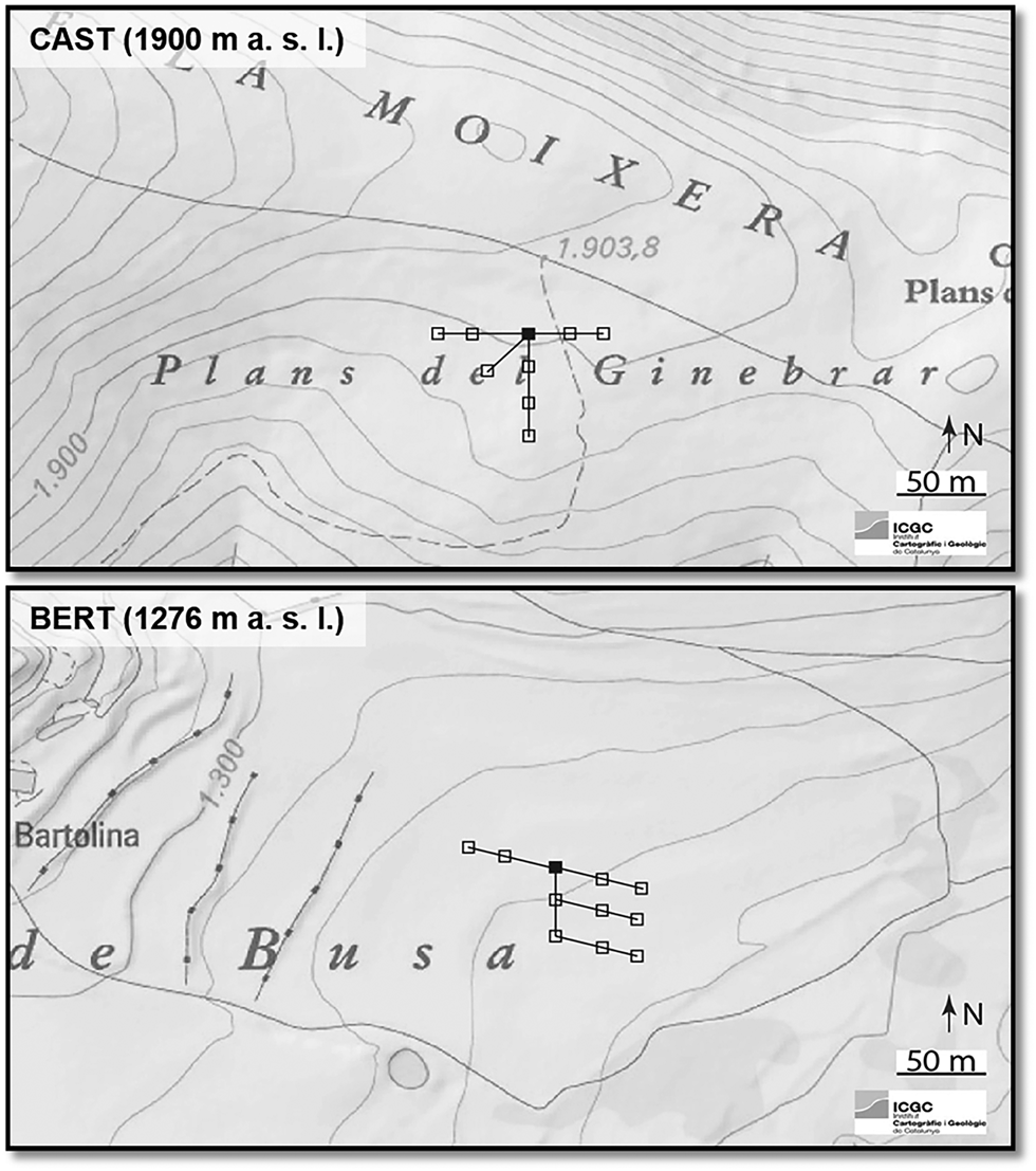
Fig. 2. Map of the study sites, Bertolina (BERT) and Castellar (CAST), and scheme of the seasonal sampling design. White blocks: sampling points, black blocks: eddy covariance stations. Every sampling day new sampling points were selected. Contour line interval 10 m.
At each sampling point, complete CO2 exchange measurements (NEE and ecosystem respiration, Reco, see CO2 exchange flux calculations) were recorded twice during daytime (08:00–16:30 UTC). After CO2 exchange measurement, total aboveground biomass was harvested at the ground level. Total aboveground biomass was separated into the different vegetation fractions: AGLB, SDB (dead biomass attached to the plant) and litter (dead plant material, detached from the plant and on the soil surface) to characterize vegetation phenological changes. Dry weight (DW, g/m2) of all vegetation fractions was determined after oven drying at 60 °C until constant weight.
The aim of the diel sampling was to assess the effect of the dominant PFT on NEE, via the PFT-specific light response. A campaign of intensive CO2 exchange measurements was carried out at each site, coinciding with the peak biomass (end of May at BERT, day of year (DOY) 150–152 and end of June at CAST, DOY 172–173), to reduce the variability related to different phenological stages and/or environmental conditions, and focusing on the effect of the PFT dominance. Sampling points were selected to ensure the presence of patches with dominance of forbs (F-dominated), grasses (G-dominated) and legumes (L-dominated), selecting three replicates for each PFT (n = 9 in both sites). CO2 exchange complete measurements (NEE and Reco) were done intensively during 48 h at BERT and 24 h at CAST, resulting in 75 complete CO2 exchange measurements in BERT and 46 at CAST.
As in the seasonal sampling, total aboveground biomass was harvested after CO2 exchange measurements, and processed in the same way. However, to verify that the PFT dominance classification (F-dominated, G-dominated, L-dominated) given in the field was correct, the AGLB was separated into PFT (forbs, grasses and legumes) to determine the fraction of each PFT, after oven drying at 60 °C until constant weight.
Afterwards, the evenness index was calculated according to Kirwan et al. (Reference Kirwan, Lüscher, Sebastià, Finn, Collins, Porqueddu, Helgadottir, Baadshaug, Brophy, Coran, Dalmannsdóttir, Delgado, Elgersma, Fothergill, Frankow-Lindberg, Golinski, Grieu, Gustavsson, Höglind, Huguenin-Elie, Iliadis, Jørgensen, Kadziuliene, Karyotis, Lunnan, Malengier, Maltoni, Meyer, Nyfeler, Nykanen-Kurki, Parente, Smit, Humm and Connolly2007), which has been defined as a measure of the distribution of the relative abundance of each PFT or species, and lies between 0, for mono-specific plots, and 1 when all species or PFT are equally represented (Kirwan et al., Reference Kirwan, Lüscher, Sebastià, Finn, Collins, Porqueddu, Helgadottir, Baadshaug, Brophy, Coran, Dalmannsdóttir, Delgado, Elgersma, Fothergill, Frankow-Lindberg, Golinski, Grieu, Gustavsson, Höglind, Huguenin-Elie, Iliadis, Jørgensen, Kadziuliene, Karyotis, Lunnan, Malengier, Maltoni, Meyer, Nyfeler, Nykanen-Kurki, Parente, Smit, Humm and Connolly2007). A cluster analysis (Ward's method) was performed based on the PFT proportions and the evenness index, confirming the PFT dominance classification given in the field. Plots G-dominated had generally very low evenness and very high grass proportion, while F-dominated and L-dominated plots had higher values of evenness and the proportion of forbs and legumes, was not so high (Fig. S1).
Carbon dioxide exchange flux calculations
Carbon dioxide exchange measurements were carried out using a self-made non-steady state chamber, connected to an infrared gas analyser (LI-840, LI-COR, USA). Resulting CO2 mixing ratios (ppm) were recorded at five seconds intervals by a laptop computer connected to the gas analyser (Fig. 3).
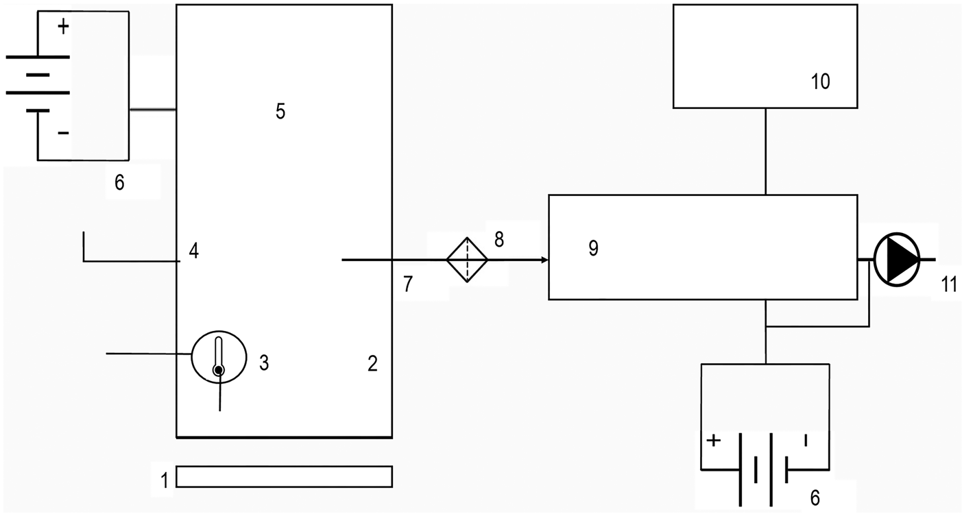
Fig. 3. Scheme of the gas-exchange measurement system set-up. (1) metal collars (height = 8 cm, inner diameter = 25 cm), hammered into the soil around 3 weeks before to let the system recover from the disturbance; (2) methacrylate chamber (height = 38.5 cm, inner diameter = 25 cm), rubber joint at its base to provide sealing at the chamber-ring junction; (3) multi-logger thermometer (TMD-56, Amprove, USA); (4) vent to avoid under pressure inside the chamber (Davidson et al., Reference Davidson, Savage, Verchot and Navarro2002); (5) fan to homogenize the air in the headspace; (6) batteries; (7) polyethylene liner with ethyl vinyl acetate shell tube (Bev a Line IV, longitude = 15.3 m, inner diameter = 3.175 mm); (8) air filter (pore size = 0.1 μm); (9) infrared gas analyser (LI-840, LI-COR, USA); (10) laptop and (11) air pump, output flow set at 1.67.10−5 m3/s, which is 1 l/min.
Carbon dioxide exchange measurements were performed closing the chamber during 30 s in light conditions (NEE), and shading the chamber to create dark conditions (Reco). GPP was estimated as the sum of both fluxes. Prior to flux calculation, mixing ratios were converted to molar densities (in mol/m3, termed as concentration in what follows) using the ideal gas law. Afterwards, CO2 fluxes were calculated based on the concentration change, following the mass balance equation (Eqn (1), Altimir et al., Reference Altimir, Vesala, Keronen, Kulmala and Hari2002):

where q is the air flow rate (1.67 10−5 m3/s, which is 1 litres/min), Ca the atmospheric CO2 concentration, Ct the CO2 concentration inside the chamber at time t (s), V the chamber volume (0.019 m3), A the sampling surface (0.049 m2) and (dC/dt) the first derivative of the CO2 concentration in relation to time (mol m3/s). Fluxes from the atmosphere to the biosphere were considered negative, and from the biosphere to the atmosphere positive, according to the micrometeorological sign convention.
Finally, data quality was checked based on the flux detection limit, calculated from the standard deviation of the ambient concentration observed over the measuring time, and on linearity (R 2) of the concentration change during the chamber closure. Fluxes with an adjusted R 2 < 0.8 and/or below the detection limit were excluded from further analysis (Debouk et al., Reference Debouk, Altimir and Sebastià2018).
In addition, the eddy covariance flux stations previously installed at each site provided 30 min averaged meteorological data used in the site description (see Study sites section) and CO2 exchange modelling (see Data analysis section): air temperature (Ta, HMP45C, Vaisala Inc, Helsinki, Finland); volumetric soil water content at 5 cm depth (SWC, CS616, Campbell Scientific, Logan UT, USA); photosynthetically active radiation (PAR, SKP215, Skye Instruments Ltd, Powys, UK) and normalized difference vegetation index, calculated as NDVI = (NIR − Red)/(NIR + Red), where ‘Red’ and ‘NIR’ are the spectral reflectance measurements acquired in the red and near-infrared regions, respectively.
Data analysis
Seasonal carbon dioxide dynamics
All data analyses were performed using the R software (R core Team, Reference R Core Team2015). To describe seasonal CO2 dynamics, average daytime CO2 exchange fluxes were calculated using data obtained between 8:00 and 16:30 UTM. To investigate the influence of phenology and environmental variables on CO2 exchange fluxes in the two climatically contrasted grasslands, linear models were run with the given CO2 flux (NEE, GPP or Reco), as function of vegetation fractions (AGLB, SDB and litter) as a proxy of phenological changes, and abiotic variables (Ta, SWC, PAR), in interaction with site (Eqn (2)). The inclusion of ‘site’ into the model incorporated the variability due to each specific grassland do not assume by the rest of explanatory variables, such as management for instance.

Collinearity among variables was tested by the variance inflation factors (VIF) tests, using the vif function, car package (Fox and Weisberg, Reference Fox and Weisberg2011). Collinearities between variables were found to be not relevant (VIF < 5, Zuur et al., Reference Zuur, Ieno and Smith2007). Final models were selected by a stepwise procedure based on the Akaike information criterion (AIC) using the stepAIC function, MASS package (Venables and Ripley, Reference Venables and Ripley2002). The relative importance of each predictive variable was determined by the calc.relimp function, relaimpo package (Groemping, Reference Groemping2006).
Plant functional type dominance on net ecosystem exchange light response
To assess the influence of PFT dominance on NEE, the NEE v. PAR relationship was modelled using a logistic sigmoid light response function (Eqn (3), Moffat, Reference Moffat2012).

where GPPsat is the asymptotic GPP, α is the apparent quantum yield, defined as the initial slope of the light-response curve and Reco,day the average daytime ecosystem respiration (Eqn (3)). Two variants of NEE v. PAR relationships were fitted: (1) using .flux densities per grassland ground area (NEE, μmol CO2/m2/s) and (2) using NEE normalized by AGLB (NEEAGLB, μmol CO2/g/s).
Afterwards, the PFT dominance effect was tested on light response parameters in both cases, using nonlinear mixed-effects models (Pinheiro and Bates, Reference Pinheiro and Bates2000), by the nlme function of the nlme package (Pinheiro et al., Reference Pinheiro, Bates, DebRoy and Sarkar2015). For that purpose, null models in each case (NEE ~ PAR, Model 1.1, and NEEAGLB~ PAR, Model 2.1) were performed, with site as a random factor and light response parameters (Eqn (3): α, GPPsat and Reco,day) as fixed effects. Afterwards, corresponding models with PFT dominance as covariates of the parameters, α, GPPsat and Reco,day (Model 1.2 and Model 2.2) were also run. Null models and models including PFT dominance as covariates were compared by an analysis of variance (ANOVA).
Results
Seasonal carbon dioxide flux dynamics in montane and subalpine grasslands
Mean daytime NEE was mostly dominated by assimilation at both sites, ranging from −2 ± 1 to −10 ± 2 μmol CO2/m2/s at BERT, and from 2 ± 1 to −20 ± 3 μmol CO2/m2/s at CAST. Mean daytime GPP showed the strongest seasonal pattern and the highest differences between sites, ranging from −5 ± 1 to −20 ± 2 μmol CO2/m2/s at BERT and form −6 ± 1 to −32 ± 2 μmol CO2/m2/s at CAST. Finally, mean daytime Reco ranged from 3.0 ± 0.4 to 10 ± 1 μmol CO2/m2/s at BERT and from 3.1 ± 0.5 to 15 ± 5 μmol CO2/m2/s at CAST (Fig. 4(a)).
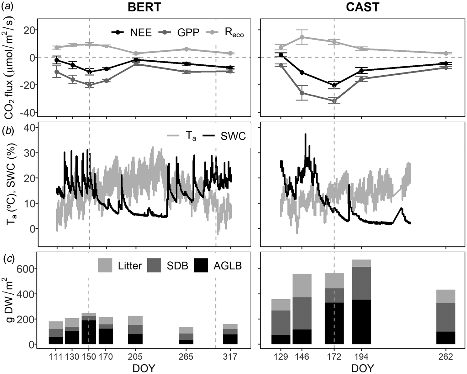
Fig. 4. Seasonal dynamics (DOY): (a) Mean daytime CO2 exchange fluxes: net ecosystem exchange (NEE), gross primary production (GPP) and ecosystem respiration (Reco) ± standard error; (b) 30 min averaged air temperature (Ta) and volumetric soil water content (SWC) at 5 cm depth, source: eddy covariance stations. A system failure of the eddy covariance flux station at CAST caused missing meteorological data from DOY 219 up to the end of the study period and (c) mean litter, SDB and AGLB. Grey dashed vertical lines indicate the beginning and end of the grazing period.
Carbon dioxide exchange seasonal patterns (Fig. 4(a)), evolved according to environmental conditions (Fig. 4(b)) and phenology (Fig. 4(c)). The modelling showed that NEE was mainly driven by AGLB (Fig. 5), increasing net CO2 uptake – more negative NEE – with increasing AGLB (Table 1); while net CO2 uptake decreased with increasing SDB and litter (Table 1).

Fig. 5. Relative importance of explicative variables linear modelling (Table 1): AGLB, SDB, litter, air temperature (Ta), soil water content (SWC) and site, with BERT as the reference level. ‘Site x’ indicates interactions between the site and the given variable.
Table 1. Carbon dioxide (CO2) exchange linear model results
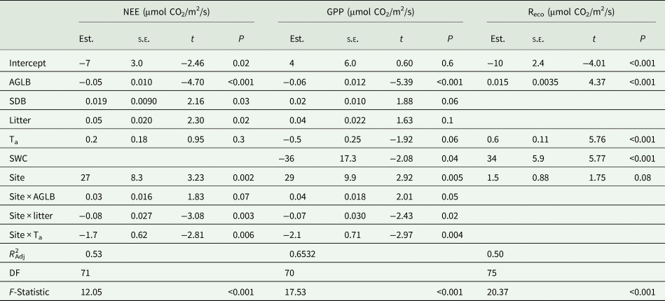
Net ecosystem exchange (NEE), gross primary production (GPP) and ecosystem respiration (Reco), as function of aboveground living biomass (AGLB), standing dead biomass (SDB), litter, air temperature (Ta), soil water content (SWC) and site, with BERT as the reference level. ‘Site x’ indicates interactions between site and the given variable. Estimates of the explanatory variables (Est.), standard error (s.e.), t and P value. Model adjusted R 2, degrees of freedom (DF) and F-statistic.
Moreover, there were some interactions between site and environmental conditions (Table 1 and Fig. 5). Net CO2 uptake was a priori lower at CAST than at BERT (less negative NEE, site effect, Table 1), and the AGLB was proportionally taking-up CO2 at lower rates at CAST than at BERT (site × AGLB, Table 1). However, net CO2 uptake increased with temperature at a higher rate at CAST than at BERT (site × Ta effect, Table 1).
GPP behaved similarly to NEE: GPP was mainly driven by AGLB (Fig. 5), increasing the gross uptake – more negative GPP – with increasing AGLB, and decreasing the gross uptake with SDB (Table 1). Gross uptake in addition increased with increasing temperature and SWC (Table 1). GPP presented the same interactions between site, environmental variables and vegetation as NEE did (Table 1). Finally, Reco was also mainly driven by AGLB (Fig. 5), increasing emissions with AGLB, followed by temperature, and SWC (Table 1).
Plant functional type dominance on net ecosystem exchange light response
CO2 exchange fluxes recorded during the intensive diel campaign confirmed that NEE was mainly driven by PAR at a diel timescale (Fig. 6). The logistic sigmoid light response function (Eqn (3)) explained 69% of the variability, when assessing NEE per grassland ground area (Model 1.1, Table 2).

Fig. 6. Observed NEE (points) v. predicted NEE (line) by the logistic sigmoid light response function (Eqn (3)) per site and per PFT dominance –forbs dominated (F-dominated), grasses dominated (G-dominated) and legumes dominated (L-dominated) – based on (a) NEE per unit of grassland ground area (NEE μmol CO2/m2/s) and (b) NEE per unit of AGLB (NEEAGLB μmol CO2/g/s).
Table 2. Nonlinear mixed-effects models results, by the logistic sigmoid light response function (Eqn (3))
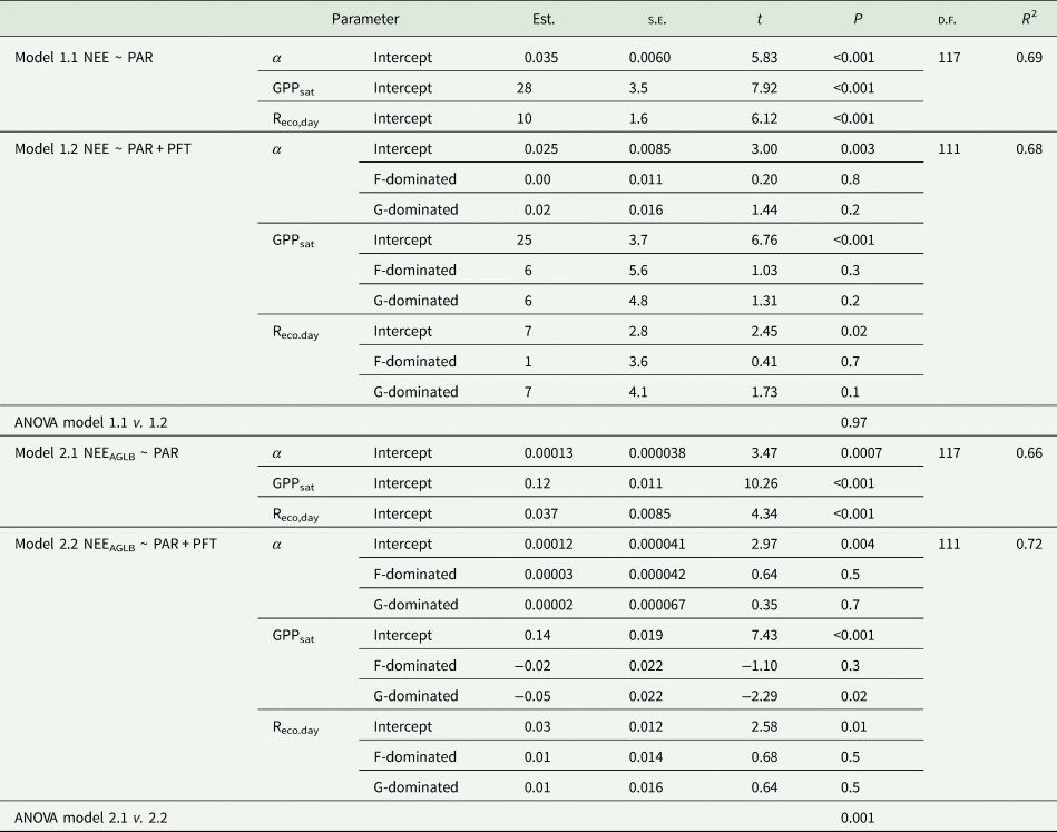
Net ecosystem exchange (NEE) as a function of photosynthetically active radiation (PAR): (1) NEE ~ PAR per grassland ground area (NEE, μmol CO2/m2/s) and (2) NEE normalized by living biomass (NEEAGLB, μmol CO2/g/s). Models 1.1 and 2.1 (null models), parameters as fixed effects: quantum yield (α), asymptotic gross primary production (GPPsat) and daytime ecosystem respiration (Reco,day). Models 1.2 and 2.2 plant functional type (PFT) dominance as covariates. PFT dominance with L-dominated as the reference level. Estimates (Est.), standard error (s.e.), t and P value. Model R 2, degrees of freedom (DF) and ANOVAs comparing models.
The inclusion of PFT dominance as covariates of the light response function parameters (α, GPPsat and Reco,day), was not significant when assessing NEE per grassland ground area (Model 1.2, Table 2). However, the logistic sigmoid adjustment per site and per PFT dominance suggested that there were differences between PFT when assessing the NEE per unit of AGLB (NEEAGLB, Fig. 6(b)). Accordingly, when assessing the NEEAGLB ~ PAR relationship, there were significant differences between the null model and the model that included PFT dominance as covariate of the parameters (ANOVA Model 2.1 v. Model 2.2, Table 2), which also increased the explained variability, from 0.66 to 0.72 (R 2 Model 2.1 v. Model 2.2, Table 2). Differences among PFT in the NEEAGLB were mainly driven by differences in the GPPsat, G-dominated plots having significantly lower GPPsat than L-dominated plots (Model 2.2, Table 2).
Discussion
Differential contributions of phenology and environmental variables on carbon dioxide seasonal dynamics between elevation belts
Contextualizing recorded CO2 exchange fluxes (Fig. 4(a)), they were higher than in other seminatural grasslands in the Pyrenees previously reported (Gilmanov et al., Reference Gilmanov, Soussana, Aires, Allard, Ammann, Balzarolo, Barcza, Bernhofer, Campbell, Cernusca, Cescatti, Clifton-Brown, Dirks, Dore, Eugster, Fuhrer, Gimeno, Gruenwald, Haszpra, Hensen, Ibrom, Jacobs, Jones, Lanigan, Laurila, Lohila, Manca, Marcolla, Nagy, Pilegaard, Pinter, Pio, Raschim, Rogiers, Sanz, Stefanim, Sutton, Tuba, Valentini, Williams and Wohlfahrt2007, Reference Gilmanov, Aires, Barcza, Baron, Belelli, Beringer, Billesbach, Bonal, Bradford, Ceschia, Cook, Corradi, Frank, Gianelle, Gimeno, Gruenwald, Guo, Hanan, Haszpra, Heilman, Jacobs, Jones, Johnson, Kiely, Li, Magliulo, Moors, Nagy, Nasyrov, Owensby, Pinter, Pio, Reichstein, Sanz, Scott, Soussana, Stoy, Svejcar, Tuba and Zhou2010; Wohlfahrt et al., Reference Wohlfahrt, Anderson-Dunn, Bahn, Berninger, Campbell, Carrara, Cescatti, Christensen, Dore, Friborg, Furger, Gianelle, Hargreaves, Hari, Haslwanter, Marcolla, Milford, Nagy, Nemitz, Rogiers, Sanz, Siegwolf, Susiluoto, Sutton, Tuba, Ugolini, Valentini, Zorer and Cernusca2008a; Sjögersten et al., Reference Sjögersten, Llurba, Ribas, Yanez-Serrano and Sebastià2012).
For instance, Gilmanov et al. (Reference Gilmanov, Soussana, Aires, Allard, Ammann, Balzarolo, Barcza, Bernhofer, Campbell, Cernusca, Cescatti, Clifton-Brown, Dirks, Dore, Eugster, Fuhrer, Gimeno, Gruenwald, Haszpra, Hensen, Ibrom, Jacobs, Jones, Lanigan, Laurila, Lohila, Manca, Marcolla, Nagy, Pilegaard, Pinter, Pio, Raschim, Rogiers, Sanz, Stefanim, Sutton, Tuba, Valentini, Williams and Wohlfahrt2007) reported in Alinyà, a montane grassland (1770 m a.s.l) that might be climatically comparable to BERT, maximum daily aggregated GPP of −25.7 g CO2/m2/day. Whereas in BERT, considering the light response function (Eqn (3)), the estimates of the parameters subtracted from the NEEAGLB ~ PAR relationship (Table 2, Model 2.1), and the AGLB sampled during the peak biomass (190 ± 21 g DW/m2, DOY 150, Fig. 4(c)), maximum daily aggregated GPP can be estimated ≈ −31 g CO2/m2/day. Such difference may well be because there are important vegetation differences between both sites, with a maximum productivity at Alinyà around 131 ± 12 g DW/m2 (unpublished data), while at BERT it is roughly a 45% higher (190 ± 21 g DW/m2), although other factors, as for instance soil differences – soil at Alinyà is a lithic cryrendoll (Gilmanov et al., Reference Gilmanov, Soussana, Aires, Allard, Ammann, Balzarolo, Barcza, Bernhofer, Campbell, Cernusca, Cescatti, Clifton-Brown, Dirks, Dore, Eugster, Fuhrer, Gimeno, Gruenwald, Haszpra, Hensen, Ibrom, Jacobs, Jones, Lanigan, Laurila, Lohila, Manca, Marcolla, Nagy, Pilegaard, Pinter, Pio, Raschim, Rogiers, Sanz, Stefanim, Sutton, Tuba, Valentini, Williams and Wohlfahrt2007), while the soil at BERT is a udic calciustept – may also be influencing.
Another example is the CO2 exchange fluxes reported by Sjögersten et al. (Reference Sjögersten, Llurba, Ribas, Yanez-Serrano and Sebastià2012) in a subalpine grassland of the southeaster Pyrenees, very close to our subalpine site CAST. They reported maximum NEE values of −0.7 ± 0.8 μmol CO2/m2/s in June, while our NEE in a similar date (DOY 172, −20 ± 3 μmol CO2/m2/s, Fig. 4(a)) amply exceed this value. Such a huge difference is only realistic if it is the result of a large difference in AGLB between both grasslands, possibly in combination with different phenological development stages and grazing pressure. Sjögersten et al. (Reference Sjögersten, Llurba, Ribas, Yanez-Serrano and Sebastià2012) reported in June an AGLB of 107 ± 15 g DW/m2, while in our site CAST we had 330 ± 40 g DW/m2 in late June (+210%, DOY 172, Fig. 4(c)), reaching the peak biomass around that date. Indeed, the AGLB reported by Sjögersten et al. (Reference Sjögersten, Llurba, Ribas, Yanez-Serrano and Sebastià2012) in June is more similar to our value in late May (DOY 146, 116 ± 33 g DW/m2, Fig. 4(c)). These differences reveal how dynamic those grasslands are, and exemplify the need for a better understanding of CO2 drivers in mountain ecosystems to perform accurate predictions and upscaling.
In line with this dynamism, the current results emphasize the role that phenology plays as an important factor influencing CO2 exchange fluxes. The well-known effect of AGLB as a CO2 exchange driver was clear, but the relevance of other vegetation fractions, including SDB and litter, which lowered the gross and net CO2 uptake capacity of the ecosystem (Table 1 and Fig. 5) was important.
Moreover, there were interesting interactions between site, phenology and environmental variables. On one hand, the AGLB at the subalpine grassland, CAST, was proportionally taking-up CO2 at lower rates than at the montane grassland BERT; resulting in proportionally lower rates of NEE per unit of AGLB (site × AGLB effect on NEE, Table 1). This suggests that environmental conditions were more constraining in CAST than at BERT, and vegetation at CAST could proportionally photosynthesize at lower rates than at BERT. However, although CAST was probably more temperature limited, the gross and net CO2 uptake capacity increased more markedly in CAST than at BERT as soon as temperatures increased (site × Ta effect on NEE and GPP, Table 1).
Accordingly, some ecosystem functions, including biomass production and CO2 exchange, in high elevation mountain grasslands have been reported to be more temperature-limited than water-limited (Sebastià, Reference Sebastià2007), being mostly constrained to the warm months. Thus, the pronounced gross and net CO2 uptake with vegetation development at CAST (Fig. 4), is in line with the fact that in the Mediterranean region high-elevation grasslands are generally highly productive during the summer, while montane grasslands have a longer growing season but less productive (García-González, Reference García-González2008). In fact, these phenological differences describe their managing use.
On the other hand, there were important site differences in the way that SWC drove GPP and Reco (Fig. 4), partly related to phenological differences between both elevations and vegetation development strategies. SWC enhanced both gross CO2 uptake and release fluxes (Table 1), in agreement with earlier works (Law et al., Reference Law, Falge, Gu, Baldocchi, Bakwin, Berbigier, Davis, Dolman, Falk, Fuentes, Goldstein, Granier, Grelle, Hollinger, Janssens, Jarvis, Jensen, Katul, Mahli, Matteucci, Meyers, Monson, Munger, Oechel, Olson, Pilegaard, Paw U, Thorgeirsson, Valentini, Verma, Vesala, Wilson and Wofsy2002; Flanagan and Johnson, Reference Flanagan and Johnson2005; Davidson and Janssens, Reference Davidson and Janssens2006; Bahn et al., Reference Bahn, Rodeghiero, Anderson-Dunn, Dore, Gimeno, Drösler, Williams, Ammann, Berninger, Flechard, Jones, Balzarolo, Kumar, Newesely, Priwitzer, Raschi, Siegwolf, Susiluoto, Tenhunen, Wohlfahrt and Cernusca2008; Imer et al., Reference Imer, Merbold, Eugster and Buchmann2013). However, when the SWC dropped, CO2 exchange fluxes diminished especially at BERT, while that diminishment at CAST was not so pronounced. Hence, although the SWC during the peak-biomass was clearly lower at CAST than at BERT (Fig. 4(b), SWC below 10% indicates a dry period), the low SWC did not cause an immediate decrease of the CO2 exchange fluxes at CAST (Fig. 4(a)).
This may well be because CAST had high SWC during the spring, which allowed the development of the vegetation once the temperature increased (Fig. 4). The well-developed AGLB was able to cope with the SWC deficit during the summer drought, and GPP and Reco did not decrease at CAST as much as at BERT. This suggests that BERT was probably more water-limited than CAST, in agreement with some studies that have highlighted that summer drought effects on productivity (Gilgen and Buchmann, Reference Gilgen and Buchmann2009) and CO2 assimilation (Bollig and Feller, Reference Bollig and Feller2014) may be more intense at sites with lower annual precipitation, as is the case of BERT in comparison with CAST.
Accordingly, vegetation may be adopting different development strategies between sites. Plants at CAST may be taking a ‘water spending strategy’ (Leitinger et al., Reference Leitinger, Ruggenthaler, Hammerle, Lavorel, Schirpke, Clement, Lamarque, Obojes and Tappeiner2015), meaning that some of the typical grassland species may not regulate the stomatal conductance until SWC approaches the wilting point under occasional droughts (Brilli et al., Reference Brilli, Hörtnagl, Hammerle, Haslwanter, Hansel, Loreto and Wohlfahrt2011). However, it must be considered that long term changes in water availability would finally lead to shifts in vegetation composition towards more opportunistic species in perennial alpine and subalpine grasslands (Sebastià, Reference Sebastià2007; Debouk et al., Reference Debouk, De Bello and Sebastia2015).
Also, CAST has a less stony soil, which allows the development of a more complex radicular system (mean belowground biomass in the first 20 cm at the peak biomass stage in 2012: BERT, 730 and CAST, 3158 g DW/m2, unpublished data), which could be offsetting the superficial SWC deficit.
Ultimately, the inclusion of site could be acting as a proxy of the intrinsic characteristics of each altitudinal belt (montane v. subalpine), including information of complex interactions between biotic and abiotic variables, as well as current and past management practices (Leifeld et al., Reference Leifeld, Meyer, Budge, Sebastia, Zimmermann and Fuhrer2015).
Finally, AGLB was also an important driver of Reco (Table 1 and Fig. 5), indicating that CO2 release was most likely dominated by the autotrophic than by the heterotrophic component of Reco. In agreement, it has been reported that the magnitude of Reco components changes considerably over the year in grassland ecosystems, and the autotrophic respiration reaches its maximum during the growing season (Gomez-Casanovas et al., Reference Gomez-Casanovas, Matamala, Cook and Gonzalez-Meler2012).
Plant functional type dominance on net ecosystem exchange light response
PFT dominance influenced on the NEE light response, when accounting for NEEAGLB (Model 2.2, Table 2). Grass dominated (G-dominated) plots had lower GPPsat, than plots dominated by legumes. This is in agreement with previous studies that have reported that legumes yield higher CO2 exchange rates than forbs and grasses, per unit of biomass (Reich et al., Reference Reich, Buschena, Tjoelker, Wrage, Knops, Tilman and Machado2003). Such differences in CO2 exchange rates between PFT dominance groups are most likely related to identity effects regarding the ecophysiological characteristics of each PFT. Legumes have the ability to fix atmospheric nitrogen (e.g. Reich et al., Reference Reich, Buschena, Tjoelker, Wrage, Knops, Tilman and Machado2003, Reference Reich, Walters and Ellsworth1997) and have higher leaf nitrogen content, which results in higher photosynthetic capacity and CO2 uptake (Reich et al., Reference Reich, Walters and Ellsworth1997, Reference Reich, Ellsworth and Walters1998; Lee et al., Reference Lee, Reich and Tjoelker2003; Busch et al., Reference Busch, Sage and Farquhar2018). In addition, legumes have higher specific leaf area than grasses, a trait that has been related to increased photosynthesis rates (Reich et al., Reference Reich, Ellsworth and Walters1998).
However, L-dominated plots tended to have lower AGLB than G-dominated and F-dominated plots (Fig. S2), and although G-dominated plots had lower GPPsat, resulting in lower NEEAGLB than L-dominated plots (Fig. 6(b)), their higher biomass offset this difference at the grassland ground scale (Model 1.2, Table 2). In this regard, previous studies showed that different PFT have different strategies to produce and maintain their biomass and access resources (Craine et al., Reference Craine, Tilman, Wedin, Reich, Tjoelker and Knops2002). Legumes access nitrogen to avoid nutrient limitation and produce high-nitrogen biomass, while grasses and forbs produce low-nitrogen biomass. Low-nitrogen species, especially grasses, have lower rates of physiological activity but generate dense and long-lived tissues that result in more biomass in the long term compared to high-nitrogen species, as is the case of legumes (Craine et al., Reference Craine, Tilman, Wedin, Reich, Tjoelker and Knops2002). Moreover, symbiotic fixation of atmospheric nitrogen by legumes requires additional energy in comparison with nitrogen acquisition from the soil (Postgate, Reference Postgate1998; Minchin and Witty, Reference Minchin, Witty, Lambers and Ribas-Carbo2005), causing more investment of photosynthates in the nitrogen fixation processes.
In addition, apart from the effects referable to the identity effects of each PFT, possible interactions between PFT must be considered. L-dominated plots had higher evenness than G-dominated plots (Fig. S1), meaning that L-dominated plots had higher functional diversity. Hence, functional diversity and PFT interactions may be producing an enhancement of the CO2 exchange per unit of biomass in addition to the rates of each single PFT. This would be in agreement with the ‘complementarity hypothesis’, which postulates that trait dissimilarity among species or PFT maximizes resource use strategies and ecosystem functioning (Tilman et al., Reference Tilman, Lehman and Thomson1997). Several studies have reported diversity and compositional effects, mainly due to grass–legume interactions on several ecosystem functions, including CO2 exchange, yield and/or nitrogen availability (Nyfeler et al., Reference Nyfeler, Huguenin-Elie, Suter, Frossard, Connolly and Lüscher2009, Reference Nyfeler, Huguenin-Elie, Suter, Frossard and Lüscher2011; Finn et al., Reference Finn, Kirwan, Connolly, Sebastià, Helgadottir, Baadshaug, Bélanger, Black, Brophy, Collins, Čop, Dalmannsdóttir, Delgado, Elgersma, Fothergill, Frankow-Lindberg, Ghesquiere, Golinska, Golinski, Grieu, Gustavsson, Höglind, Huguenin-Elie, Jørgensen, Kadziuliene, Kurki, Llurba, Lunnan, Porqueddu, Suter, Thumm and Lüscher2013; Ribas et al., Reference Ribas, Llurba, Gouriveau, Altimir, Connolly and Sebastià2015). For instance, Ribas et al. (Reference Ribas, Llurba, Gouriveau, Altimir, Connolly and Sebastià2015) found the highest CO2 respiration rates in plots dominated by legumes with a certain proportion of grasses, and a positive effect of evenness on respiration, verifying and disaggregating a coupled effect of the dominant PFT from PFT interaction (evenness) effects.
In our study case, dominance and interaction effects cannot be disentangled, but certainly PFT composition was influencing NEEAGLB (Model 2.2, Table 2), via PFT-specific light response differences, in seminatural mountain grasslands.
Conclusions
Phenology plays an important role as a CO2 exchange driver at the seasonal scale, driving differences between elevation belts (montane v. subalpine). Although the subalpine grassland (CAST) had a later vegetation development, CAST was clearly more productive (AGLB ~ + 74%) than the montane grassland (BERT) during the peak biomass stage, and yielded higher NEE values (NEE ~ + 48%). Thus, at least in mountain environments, detailed information on phenology is key to understand the a priori counterintuitive finding that a high-elevation grassland (CAST) is more productive than a comparable grassland at the montane elevation (BERT), with a longer growing season and warmer summer temperature. There were elevation differences in the way that environmental variables and phenology mediated CO2 exchange fluxes. Although CAST was more temperature constrained, temperature enhanced gross and net CO2 uptake at higher rates at CAST than at BERT. Also, both grasslands experienced a pronounced summer dry period, which substantially reduced productivity at the lower elevation, from which only a minor recovery could be observed in autumn. However, the delayed phenology at the subalpine grassland reduced vegetation's sensitivity to summer dryness, which did not experience a reduction in CO2 exchange, even though the low SWC.
Moreover, vegetation composition, in terms of PFT, influenced on the CO2 exchange. Legume dominated plots presented higher NEE rates than grass dominated plots per unit of AGLB; with higher GPPsat than grass dominated plots. Overall, a deeper knowledge of phenology and vegetation ecophysiological responses under different climatic conditions is key to upscale CO2 exchange fluxes in a seasonal and inter-annual scale in seminatural mountain grasslands.
Supplementary material
The supplementary material for this article can be found at https://doi.org/10.1017/S0021859620000179.
Acknowledgements
Thanks to all the colleagues who collaborated in laboratory and fieldwork tasks: Helena Sarri, Haifa Debouk, Cristina Rota, Fabrice Gouriveau, Carla Bellera and Dafne Padrós.
Financial support
The current study was developed within the project CAPACITI supported by a Marie Curie Intra European Fellowship within the 7th European Community Framework for Nuria Altimir (PIEF-GA-2010-275855) and the project BIOGEI (CGL2013-49142-C21-R) supported by a FPI fellowship for Mercedes Ibáñez (BES-2014-069243) funded by the Spanish Science Foundation (FECYT).
Conflict of interest
The authors declare there are no conflicts of interest.
Ethical standards
Not applicable.


