Feasibility of Estimating Turbulent Heat Fluxes via Variational Assimilation of Reference-Level Air Temperature and Specific Humidity Observations


Abstract
:
1. Introduction
2. Materials and Methods
2.1. Sensible and Latent Heat Fluxes
2.2. Atmospheric Boundary Layer (ABL) Model
2.2.1. Energy and Moisture Budget Equations
2.2.2. Radiative Fluxes
2.2.3. Mixed-Layer Height
2.2.4. Inversion Strengths of and
2.2.5. Entrainment Fluxes
2.3. Variational Data Assimilation (VDA) Approach
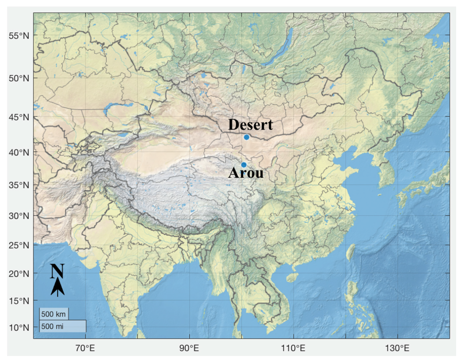
3. Study Sites
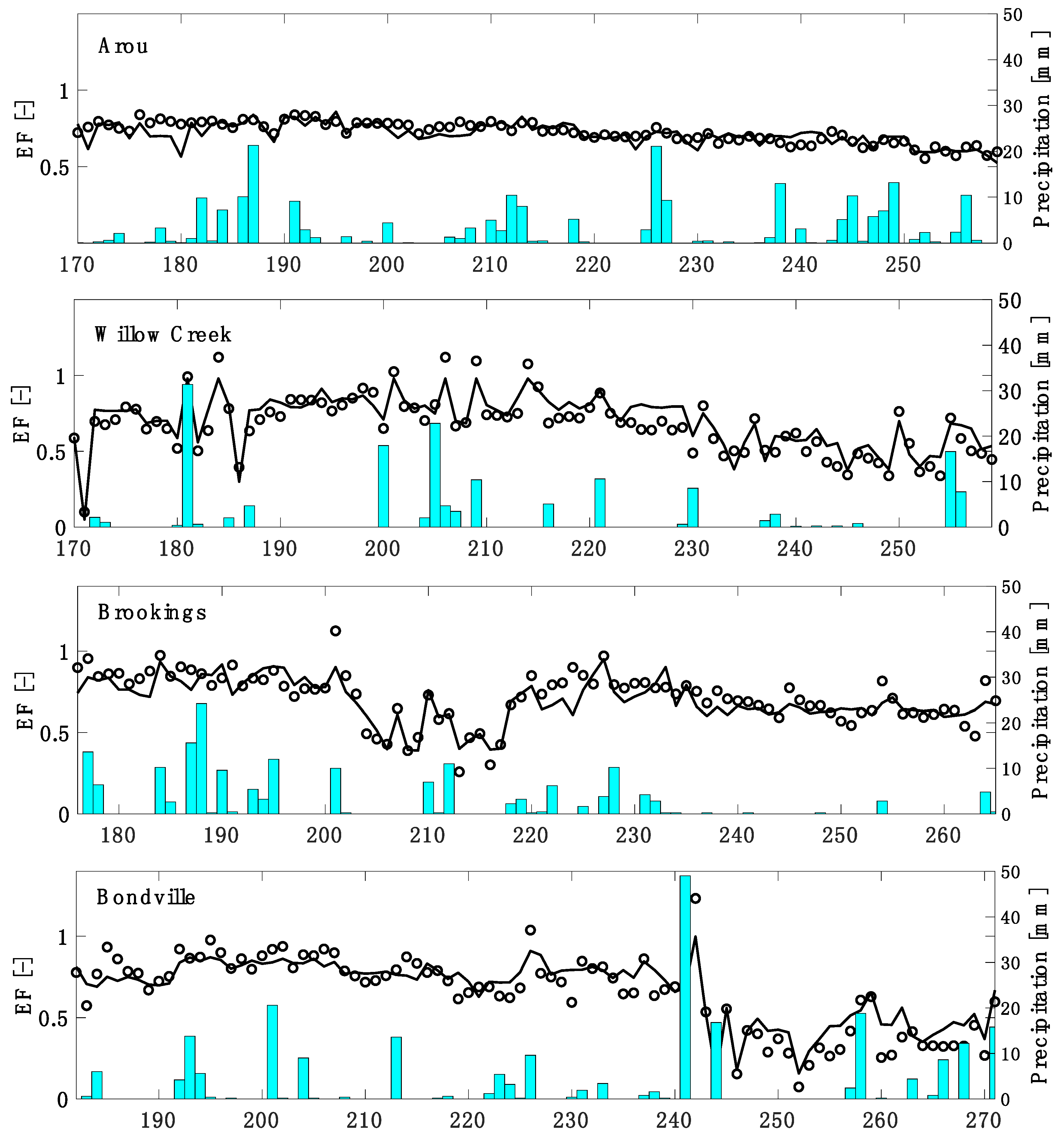
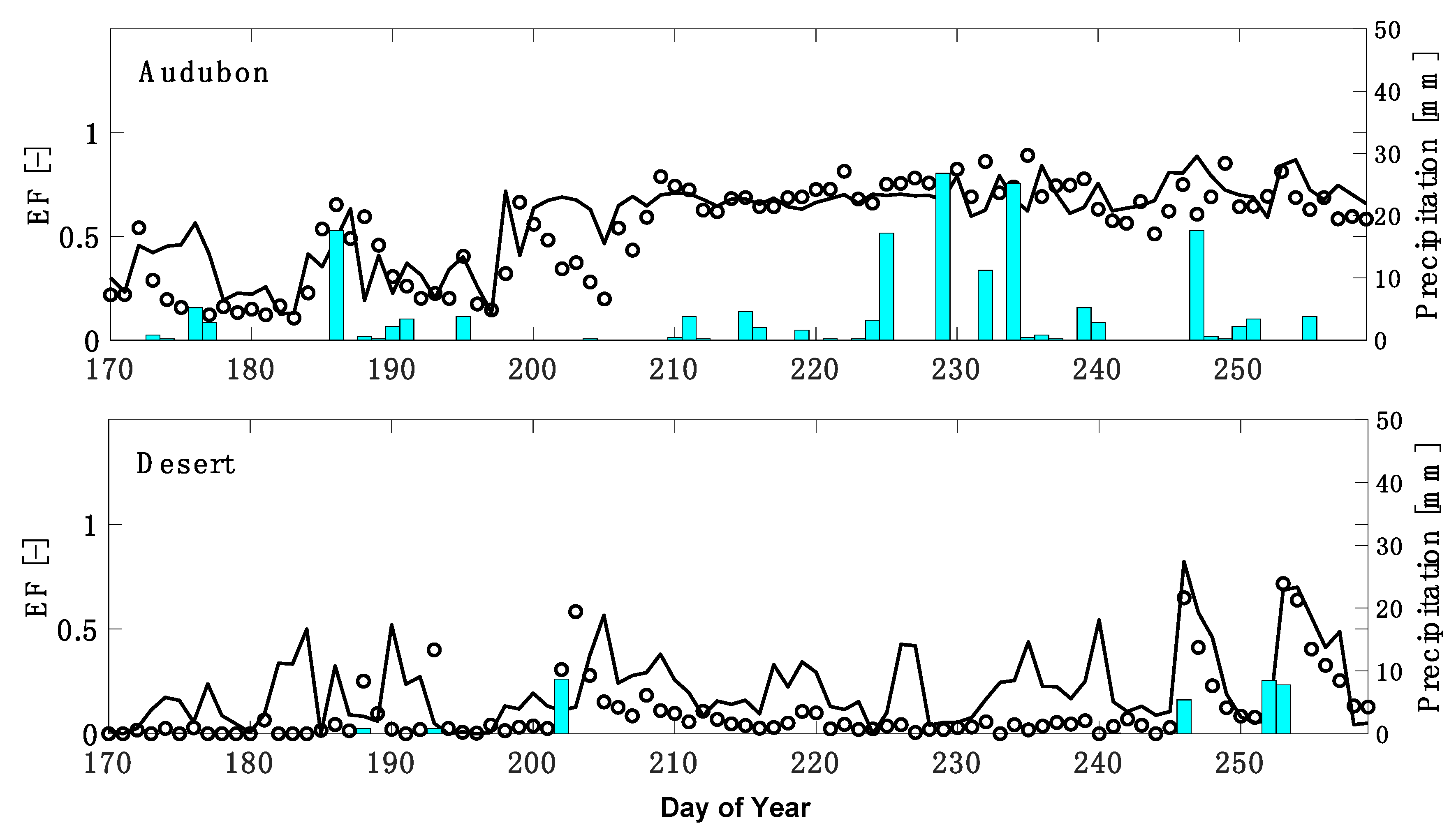
4. Results and Discussions
5. Conclusions
Author Contributions
Funding
Acknowledgments
Conflicts of Interest
Appendix A. List of symbols
| B | Stanton number | [-] |
| inverse background error covariance of | [-] | |
| inverse background error covariance of | [-] | |
| CHN | neutral bulk heat transfer coefficient | [-] |
| cp | specific heat capacity of dry air | [J kg−1 K−1] |
| dissipation of mechanical turbulent energy | [m3 s−3] | |
| d | zero-plane displacement height | [m] |
| E | evaporative rate from ground | [kg m−2 s−1] |
| EF | evaporative fraction | [-] |
| atmospheric stability correction function | [-] | |
| ground heat flux | [W m−2] | |
| production of mechanical turbulent energy | [m3 s−3] | |
| g | gravitational acceleration | [m s−2] |
| sensible heat flux | [W m−2] | |
| entrainment sensible heat flux | [W m−2] | |
| virtual heat flux | [W m−2] | |
| mixed-layer height | [m] | |
| J | objective functional | [-] |
| von Karman’s constant | [-] | |
| empirical constant | [kg m−2]−1/7 | |
| L | Monin-Obhukov length | [m] |
| latent heat of vaporization | [J kg−1] | |
| latent heat flux | [W m−2] | |
| entrainment latent heat flux | [W m−2] | |
| LAI | leaf area index | [m2 m−2] |
| m | constant | [-] |
| number of days in the assimilation period | ||
| pressure at height h | [Pa] | |
| surface pressure | [Pa] | |
| mixed layer specific humidity (equation 5b) | [kg kg−1] | |
| specific humidity at the reference-level | [kg kg−1] | |
| specific humidity immediately above mixed layer | [kg kg−1] | |
| specific humidity at the bottom of mixed layer (equation B2) | [kg kg−1] | |
| R | transformation variable | [-] |
| downwelling longwave radiation from within the mixed layer | [W m−2] | |
| upwelling longwave radiation from within the mixed layer | [W m−2] | |
| downwelling longwave radiation from above the mixed layer | [W m−2] | |
| gas constant for dry air | [J kg K−1] | |
| upwelling longwave radiation from ground into the mixed layer | [W m−2] | |
| Richardson number | [-] | |
| net radiation at the surface | [W m−2] | |
| incoming solar radiation | [W m−2] | |
| gas constant for water vapor | [J kg K−1] | |
| inverse error covariance of | [-] | |
| inverse error covariance of | [K−2] | |
| surface layer | [-] | |
| land surface temperature | [K] | |
| reference-level air temperature | [K] | |
| air temperature immediately above the mixed layer | [K] | |
| time | [s] | |
| wind speed at the reference-level | [m s−1] | |
| wind speed at the top of the surface layer | [m s−1] | |
| friction velocity | [m s−1] | |
| roughness length scales for heat | [m] | |
| roughness length scales for momentum | [m] | |
| surface-layer height | [m] | |
| reference-level height | [m] | |
| vegetation height | [m] | |
| surface albedo | [-] | |
| specific humidity inversion strength | [kg kg−1] | |
| potential temperature inversion strength | [K] | |
| atmospheric emissivity | [-] | |
| effective emissivity above the mixed-layer | [-] | |
| effective mixed-layer downward emissivity | [-] | |
| effective mixed-layer upward emissivity | [-] | |
| mixed-layer bulk emissivity | [-] | |
| surface emissivity | [-] | |
| lapse rate of above the mixed layer | [kg kg−1 m−1] | |
| lapse rate of above the mixed layer | [K m−1] | |
| lagrange multipliers | [-] | |
| stability function for heat | [-] | |
| stability function for momentum | [-] | |
| stability function for water vapor | [-] | |
| air density | [kg m−3] | |
| Stefan-Boltzmann constant | [W m−2 K−4] | |
| Mixed layer potential temperature (equation 5a) | [K] | |
| reference-level potential temperature | [K] | |
| potential temperature at the bottom of mixed layer (equation B1) | [K] | |
| mechanical turbulence dissipation parameter | [-] | |
| stability parameter | [-] |
Appendix B. Monin–Obukhov Similarity Theory (MOST)
- Guess a reasonable value for .
- Substitute from step 1 in B6 to estimate L.
- Estimate from B10.
- Substitute the estimate from the VDA approach and obtained from step 3 in B8 to find
- Substitute from step 4 in B9 to find .
- Substitute from step 5 and L from step 2 in B7 to find .
- Repeat steps 2–6 until the algorithm converges (i.e., the difference between estimates from the last two iterations becomes smaller than 0.01 m/s). This step gives us , , and estimates for a given value.
- Substitute and from step 7 in B1 and B2 to estimate and
Appendix C. Euler–Lagrange Equations
References
- McCabe, M.F.; Wood, E.F. Scale influences on the remote estimation of evapotranspiration using multiple satellite sensors. Remote Sens. Environ. 2006, 105, 271–285. [Google Scholar] [CrossRef]
- Lu, Y.; Dong, J.; Steele-Dunne, S.C.; van de Giesen, N. Estimating surface turbulent heat fluxes from land surface temperature and soil moisture observations using the particle batch smoother. Water Resour. Res. 2016, 52, 9086–9108. [Google Scholar] [CrossRef] [Green Version]
- Alfieri, J.; Kustas, W.P.; Prueger, J.H.; Chavez, J.L.; Evett, S.R.; Neals, C.; Anderson, M.; Hipps, L.; Copeland, K.; Howell, T.; et al. A comparison of the eddy covariance and lysimetry-based measurements of the surface energy fluxes during BEAREXo8. Int. Assoc. Hydrol. Sci. 2012, 352, 215–218. [Google Scholar]
- Liu, S.M.; Xu, Z.W.; Zhu, Z.L.; Jia, Z.Z.; Zhu, M.J. Measurements of evapotranspiration from eddy-covariance systems and large aperture scintillometers in the Hai River Basin, China. J. Hydrol. 2013, 487, 24–38. [Google Scholar] [CrossRef]
- Gebler, S.; Hendricks Franssen, H.-J.; Putz, T.; Post, H.; Schmidt, M.; Vereecken, H. Actual evapotranspiration and precipitation measured by lysimeters: A comparison with eddy covariance and tipping bucket. Hydrol. Earth Syst. Sci. 2015, 19, 2145–2161. [Google Scholar] [CrossRef] [Green Version]
- Hirschi, M.; Michel, D.; Lehner, I.; Seneviratne, S.I. A site-level comparison of lysimeter and eddy covariance flux measurements of evapotranspiration. Hydrol. Earth Syst. Sci. 2017, 21, 1809–1825. [Google Scholar] [CrossRef] [Green Version]
- Moorhead, J.E.; Marek, G.W.; Colaizzi, P.D.; Gowda, P.H.; Evett, S.R.; Brauer, D.K.; Marek, T.H.; Porter, D.O. Evaluation of sensible heat flux and evapotranspiration estimates using a surface layer scintillometer and a large weighing lysimeter. Sensors 2017, 17, 2350. [Google Scholar]
- Baldocchi, D.; Falge, E.; Gu, L.H.; Olson, R. FLUXNET: A new tool to study the temporal and spatial variability of ecosystem-scale carbon dioxide, water vapor, and energy flux densities. Bull. Am. Meteorol. Soc. 2001, 82, 2415–2434. [Google Scholar] [CrossRef]
- Li, X.; Cheng, G.D.; Liu, S.M.; Xiao, Q.; Ma, M.G.; Jin, R.; Che, T.; Liu, Q.; Wang, W.; Wen, J.; et al. Heihe watershed allied telemetry experimental research (HiWATER): Scientific objectives and experimental design. Bull. Am. Meteorol. Soc. 2013, 94, 1145–1160. [Google Scholar] [CrossRef]
- Xu, T.; Bateni, S.M.; Liang, S. Estimating turbulent heat fluxes with a weak-constraint data assimilation scheme: A case study (HiWATER-MUSOEXE). IEEE Geosci. Remote Sens. Lett. 2015, 12, 68–72. [Google Scholar]
- Liu, S.; Li, X.; Xu, Z.; Che, T.; Xiao, Q.; Ma, M.; Liu, Q.; Jin, R.; Guo, J.; Wang, L.; et al. The Heihe integrated observatory network: A basin-scale land surface processes observatory in China. Vadose Zone J. 2018, 17, 180072. [Google Scholar] [CrossRef]
- Bastiaanssen, W.G.M.; Menenti, M.; Feddes, R.A.; Holtslang, A.A.M. A remote sensing surface energy balance algorithm for land (SEBAL) 1. Formulation. J. Hydrol. 1998, 212, 198–212. [Google Scholar] [CrossRef]
- Bastiaanssen, W.G.M.; Pelgrum, H.; Wang, J.; MA, Y.; Moreno, J.F.; Roenrink, G.J.; Van Der Wal, T. A remote sensing surface energy balance algorithm for land (SEBAL) 2. Validation. J. Hydrol. 1998, 212, 213–229. [Google Scholar] [CrossRef]
- Kalma, J.D.; McVicar, T.R.; McCabe, M.F. Estimating land surface evaporation: A review of methods using remotely sensed surface temperature data. Surv. Geophys. 2008, 29, 421–469. [Google Scholar] [CrossRef]
- Allen, R.; Irmak, A.; Trezza, R.; Hendrickx, J.M.H.; Bastiaanssen, W.; Kjaersgaard, J. Satellite-based ET estimation in agriculture using SEBAL and METRIC. Hydrol. Process. 2011, 25, 4011–4027. [Google Scholar] [CrossRef]
- Yilmaz, M.T.; Anderson, M.C.; Zaitchik, B.; Hain, C.R.; Crow, W.T.; Ozdogan, M.; Chun, J.A.; Evans, J. Comparison of prognostic and diagnostic surface flux modeling approaches over the Nile River basin. Water Resour. Res. 2014, 50, 386–408. [Google Scholar] [CrossRef]
- Nishida, K.; Nemani, R.R.; Running, S.W.; Glassy, J.M. An operational remote sensing algorithm of land surface evaporation. J. Geophys. Res. Atmos. 2003, 108, 4270. [Google Scholar] [CrossRef]
- Wang, K.; Li, Z.; Cribb, M. Estimating of evaporative fraction from a combination of day and night land surface temperature and NDVI: A new method to determine the Priestley-Taylor parameter. Remote Sens. Environ. 2006, 102, 293–305. [Google Scholar] [CrossRef]
- Carlson, T. An overview of the “triangle method” for estimating surface evapotranspiration and soil moisture from satellite imagery. Sensors 2007, 7, 1612–1629. [Google Scholar] [CrossRef] [Green Version]
- Stisen, S.; Sandholt, I.; Nørgaard, A.; Fensholt, R.; Jensen, K.H. Combining the triangle method with thermal inertia to estimate regional evapotranspiration—Applied to MSG-SEVIRI data in the Senegal River basin. Remote Sens. Environ. 2008, 112, 1242–1255. [Google Scholar] [CrossRef]
- Tang, R.; Li, Z.-L.; Tang, B. An application of the Ts-VI triangle method with enhanced edges determination for evapotranspiration estimation from MODIS data in arid and semi-arid regions: Implementation and validation. Remote Sens. Environ. 2010, 114, 540–551. [Google Scholar] [CrossRef]
- Sun, L.; Liang, S.; Yuan, W.; Chen, Z. Improving a Penman-Monteith evapotranspiration model by incorporating soil moisture control on soil evaporation in semiarid areas. Int. J. Digit. Earth 2013, 6, 134–156. [Google Scholar] [CrossRef]
- Martínez Pérez, J.Á.; García-Galiano, S.G.; Martin-Gorriz, B.; Baille, A. Satellite-Based Method for Estimating the Spatial Distribution of Crop Evapotranspiration: Sensitivity to the Priestley-Taylor Coefficient. Remote Sens. 2017, 9, 611. [Google Scholar] [CrossRef] [Green Version]
- Majozi, N.P.; Mannaerts, C.M.; Ramoelo, A.; Mathieu, R.; Mudau, A.E.; Verhoef, W. An intercomparison of satellite-based daily evapotranspiration estimates under different eco-climatic regions in south Africa. Remote Sens. 2017, 9, 307. [Google Scholar] [CrossRef] [Green Version]
- Carlson, T.N.; Petropoulos, G.P. A new method for estimating of evapotranspiration and surface soil moisture from optical and thermal infrared measurements: The simplified triangle. Int. J. Remote Sens. 2019, 40, 7716–7729. [Google Scholar] [CrossRef]
- Zhu, W.; Jia, S.; Lv, A. A universal Ts-VI triangle method for the continuous retrieval of evaporative fraction from MODIS products. J. Geophys. Res. Atmos. 2017, 122, 206–227. [Google Scholar] [CrossRef]
- Zhang, H.; Gorelick, S.M.; Avisse, N.; Tilmant, A.; Rajsekhar, D.; Yoon, J. A New Temperature-Vegetation Triangle Algorithm with Variable Edges (TAVE) for Satellite-Based Actual Evapotranspiration Estimation. Remote Sens. 2016, 8, 735. [Google Scholar] [CrossRef] [Green Version]
- Sousa, D.; Small, C. Spectral Mixture Analysis as a Unified Framework for the Remote Sensing of Evapotranspiration. Remote Sens. 2018, 10, 1961. [Google Scholar] [CrossRef] [Green Version]
- Su, Z. The surface energy balance system (SEBS) for estimation of turbulent heat fluxes. Hydrol. Earth Syst. Sci. 2002, 6, 85–100. [Google Scholar] [CrossRef]
- Liu, S.M.; Hu, G.; Lu, L.; Mao, D.F. Estimation of regional evapotranspiration by TM/ETM + data over heterogeneous surfaces. Photogramm. Eng. Remote Sens. 2007, 73, 1169–1178. [Google Scholar] [CrossRef]
- Jia, L.; Xi, G.; Liu, S.; Huang, C.; Yan, Y.; Liu, G. Regional estimation of daily to annual regional evapotranspiration with MODIS data in the Yellow River Delta wetland. Hydrol. Earth Syst. Sci. 2009, 13, 1775–1787. [Google Scholar] [CrossRef] [Green Version]
- Kustas, W.P.; Alfieri, J.G.; Anderson, M.C.; Colaizzi, P.D.; Prueger, J.H.; Evett, S.R.; Christopher, M.U.; Andrew, N.F.; Lawrence, E.H.; Jose, L.C.; et al. Evaluating the two-source energy balance model using local thermal and surface flux observations in a strongly advective irrigated agricultural area. Adv. Water Resour. 2012, 50, 120–133. [Google Scholar] [CrossRef] [Green Version]
- Ma, W.; Hafeez, M.; Rabbani, U.; Ishikawa, H.; Ma, Y. Retrieved actual ET using SEBS model from Landsat-5 TM data for irrigation area of Australia. Atmos. Environ. 2012, 59, 408–414. [Google Scholar] [CrossRef]
- Ma, Y.F.; Liu, S.M.; Zhang, F.; Zhou, J.; Jia, Z.Z.; Song, L.S. Estimations of regional surface energy fluxes over heterogeneous oasisdesert surfaces in the middle reaches of the Heihe River during HiWATER-MUSOEXE. IEEE Geosci. Remote Sens. Lett. 2015, 12, 671–675. [Google Scholar]
- Song, L.S.; Kustas, W.P.; Liu, S.M.; Colaizzi, P.D.; Nieto, H.; Xu, Z.W.; Ma, Y.; Li, M.; Xu, T.; Agam, N.; et al. Applications of a thermal-based two-source energy balance model using Priestley-Taylor approach for surface temperature partitioning under advective conditions. J. Hydrol. 2016, 540, 574–587. [Google Scholar] [CrossRef] [Green Version]
- Mallick, K.; Jarvis, A.J.; Fisher, J.B.; Tu, K.P.; Boegh, E.; Niyogi, D. Latent heat flux and canopy conductance based on Penman-Monteith, Priestly-Taylor equation, and Bouchets complementary hypothesis. J. Hydrometeorol. 2013, 14, 419–442. [Google Scholar] [CrossRef]
- Mallick, K.; Jarvis, A.J.; Boegh, E.; Fisher, J.B.; Drewry, D.T.; Tu, K.P.; Hook, S.J.; Hulley, G.; Ardö, J.; Beringer, J.; et al. A surface temperature initiated closure (STIC) for surface energy balance fluxes. Remote Sens. Environ. 2014, 141, 243–261. [Google Scholar] [CrossRef]
- Raoufi, R.; Beighley, E. Estimating Daily Global Evapotranspiration Using Penman–Monteith Equation and Remotely Sensed Land Surface Temperature. Remote Sens. 2017, 9, 1138. [Google Scholar] [CrossRef] [Green Version]
- Peters-Lidard, C.D.; Kumar, S.V.; Mocko, D.M.; Tian, Y. Estimating evapotranspiration with land data assimilation systems, hydrological processes. Hydrol. Process. 2011, 25, 3979–3992. [Google Scholar] [CrossRef] [Green Version]
- Xia, Y.; Sheffield, J.S.; Ek, M.B.; Dong, J.; Chaney, N.; Wei, H.; Meng, J.; Wood, E.F. Evaluation of multi-model simulated soil moisture in NLDAS-2. J. Hydrol. 2014, 512, 107–125. [Google Scholar] [CrossRef]
- Xia, Y.; Ek, M.; Mocko, D.; Peters-Lidard, C.; Sheffield, J.; Dong, J.; Wood, E. Uncertainties, correlations, and optimal blends of drought indices from the NLDAS multiple land surface model ensemble. J. Hydrometeorol. 2014, 15, 1636–1650. [Google Scholar] [CrossRef]
- Bateni, S.M.; Entekhabi, D. Surface heat flux estimation with the ensemble Kalman smoother: Joint estimation of state and parameters. Water Resour. Res. 2012, 48, W08521. [Google Scholar] [CrossRef]
- Carrera, M.; Belair, S.; Bilodeau, B. The Canadian Land Data Assimilation System (CaLDAS): Description and synthetic evaluation study. J. Hydrometeorol. 2015, 16, 1293–1314. [Google Scholar] [CrossRef]
- Xu, T.; Bateni, S.M.; Neale, C.M.U.; Auligne, T.; Liang, S. Estimation of turbulent heat fluxes by assimilation of land surface temperature observations from GOES satellites into an ensemble Kalman smoother framework. J. Geophys. Res. Atmos. 2018, 123, 2409–2423. [Google Scholar] [CrossRef]
- Caparrini, F.; Castelli, F.; Entekhabi, D. Mapping of land-atmosphere heat fluxes and surface parameters with remote sensing data. Bound. Layer Meteorol. 2003, 107, 605–633. [Google Scholar] [CrossRef]
- Caparrini, F.; Castelli, F.; Entekhabi, D. Estimation of surface turbulent fluxes through assimilation of radiometric surface temperature sequences. J. Hydrometeorol. 2004, 5, 145–159. [Google Scholar] [CrossRef]
- Caparrini, F.; Castelli, F.; Entekhabi, D. Variational estimation of soil and vegetation turbulent transfer and heat flux parameters from sequences of multisensor imagery. Water Resour. Res. 2004, 40, 1713–1722. [Google Scholar] [CrossRef] [Green Version]
- Bateni, S.M.; Entekhabi, D. Relative efficiency of land surface energy balance components. Water Resour. Res. 2012, 48, W04510. [Google Scholar] [CrossRef]
- Bateni, S.M.; Entekhabi, D.; Jeng, D.-S. Variational assimilation of land surface temperature and the estimation of surface energy balance components. J. Hydrol. 2013, 481, 143–156. [Google Scholar] [CrossRef]
- Bateni, S.M.; Entekhabi, D.; Castelli, F. Mapping evaporation and estimation of surface control of evaporation using remotely sensed land surface temperature from a constellation of satellites. Water Resour. Res. 2013, 49, 950–968. [Google Scholar] [CrossRef]
- Bateni, S.M.; Entekhabi, D.; Margulis, S.; Castelli, F.; Kergoat, L. Coupled estimation of surface heat fluxes and vegetation dynamics from remotely sensed land surface temperature and fraction of photosynthetically active radiation. Water Resour. Res. 2014, 50, 8420–8440. [Google Scholar] [CrossRef] [Green Version]
- Xu, T.; Bateni, S.M.; Margulis, S.A.; Song, L.; Lio, S. Partitioning evapotranspiration into soil evaporation and canopy transpiration via a two-source variational data assimilation system. J. Hydrometeorol. 2016, 17, 2353–2370. [Google Scholar] [CrossRef]
- Xu, T.; He, X.; Bateni, S.M.; Auligne, T.; Liu, S.; Xu, Z.; Zhou, J.; Mao, K. Mapping regional turbulent heat fluxes via variational assimilation of land surface temperature data from polar orbiting satellites. Remote Sens. Environ. 2019, 221, 444–461. [Google Scholar] [CrossRef]
- Abdolghafoorian, A.; Farhadi, L. Uncertainty quantification in land surface hydrologic modeling: Toward an integrated variational data assimilation framework. IEEE J. Sel. Top. Appl. Earth Obs. Remote Sens. 2016, 9, 2628–2637. [Google Scholar] [CrossRef]
- Abdolghafoorian, A.; Farhadi, L.; Bateni, S.M.; Margulis, S.; Xu, T. Characterizing the effect of vegetation dynamics on the bulk heat transfer coefficient to improve variational estimation of surface turbulent fluxes. J. Hydrometeorol. 2017, 18, 321–333. [Google Scholar] [CrossRef]
- He, X.; Xu, T.; Bateni, S.M.; Neale, C.M.U.; Auligne, T.; Liu, S.; Wang, K.; Mao, K.; Yao, Y. Evaluation of the Weak Constraint Data Assimilation Approach for stimating Turbulent Heat Fluxes at Six Sites. Remote Sens. 2018, 10, 1994. [Google Scholar] [CrossRef] [Green Version]
- Crow, W.T.; Kustas, W.P. Utility of assimilating surface radiometric temperature observations for evaporative fraction and heat transfer coefficient retrieval. Bound. Layer Meteorol. 2005, 115, 105–130. [Google Scholar] [CrossRef]
- Xu, T.; Bateni, S.M.; Liang, S.; Entekhabi, D.; Mao, K. Estimation of surface turbulent heat fluxes via variational assimilation of sequences of land surface temperatures from Geostationary Operational Environmental Satellites. J. Geophys. Res. Atmos. 2014, 119, 10780–10798. [Google Scholar] [CrossRef] [Green Version]
- Sini, F.; Boni, G.; Caparrini, F.; Entekhabi, D. Estimation of large-scale evaporation fields based on assimilation of remotely sensed land temperature. Water Resour. Res. 2008, 44, W06410. [Google Scholar] [CrossRef]
- Abdolghafoorian, A.; Farhadi, L. Estimation of surface turbulent fluxes from land surface moisture and temperature via a variational data assimilation framework. Water Resour. Res. 2019, 55. [Google Scholar] [CrossRef]
- Mahfouf, J.-F. Analysis of soil moisture from near-surface parameters: A feasibility study. J. Appl. Meteorol. 1991, 30, 1534–1547. [Google Scholar] [CrossRef] [Green Version]
- Bouttier, F.; Mahfouf, J.F.; Noilhan, J. Sequential assimilation of soil moisture from atmospheric low-level parameters. Part I: Sensitivity and calibration studies. J. Appl. Meteorol. 1993, 32, 1335–1351. [Google Scholar] [CrossRef] [Green Version]
- Bouttier, F.; Mahfouf, J.F.; Noilhan, J. Sequential assimilation of soil moisture from atmospheric low-level parameters. II: Implementation in a mesoscale model. J. Appl. Meteorol. 1993, 32, 1352–1364. [Google Scholar] [CrossRef]
- Mahfouf, J.-F.; Viterbo, P.; Douville, H.; Beljaars, A.; Saarinen, S. A Revised land-surface analysis scheme in the Integrated Forecasting System. ECMWF Newsl. 2000, 88, 8–13. [Google Scholar]
- Mahfouf, J.-F.; Bergaoui, K.; Draper, C.; Bouyssel, F.; Taillefer, F.; Taseva, L. A comparison of two off-line soil analysis schemes for assimilation of screen level observations. J. Geophys. Res. 2009, 114, D08105. [Google Scholar] [CrossRef]
- Douville, H.; Viterbo, P.; Mahfouf, J.F.; Beljaars, A.C. Evaluation of the optimum interpolation and nudging techniques for soil moisture analysis using FIFE data. Mon. Weather Rev. 2000, 128, 1733–1756. [Google Scholar] [CrossRef]
- Hess, R. Assimilation of screen-level observations by variational soil moisture analysis. Meteorol. Atmos. Phys. 2001, 77, 145–154. [Google Scholar] [CrossRef]
- Drusch, M.; Viterbo, P. Assimilation of screen-level variables in ECMWF’s integrated forecast system: A study on the impact on the forecast quality and analyzed soil moisture. Mon. Weather Rev. 2007, 135, 300–314. [Google Scholar] [CrossRef]
- De Rosnay, P.; Drusch, M.; Vasiljevic, D.; Balsamo, G.; Albergel, C.; Isaksen, L. A simplified Extended Kalman Filter for the global operational soil moisture analysis at ECMWF. Q. J. R. Meteorol. Soc. 2013, 139, 1199–1213. [Google Scholar] [CrossRef]
- Ren, D.; Xue, M. Retrieval of land surface model state variables through assimilating screen level humidity and temperature measurements. Adv. Meteorol. 2016. [Google Scholar] [CrossRef] [Green Version]
- De Lannoy, G.J.M.; de Rosnay, P.; Reichle, R.H. Soil Moisture Data Assimilation. In Handbook of Hydrometeorological Ensemble Forecasting; Duan, Q., Pappenberger, F., Eds.; Springer: Berlin/Heidelberg, Germany, 2016. [Google Scholar]
- Holtslag, A.A.M.; Van Ulden, A.P. A single scheme for daytime estimates of the surface fluxes from routine weather data. J. Clim. Appl. Meteorol. 1983, 22, 517–529. [Google Scholar] [CrossRef]
- Margulis, S.A.; Entekhabi, D. A coupled land surface-boundary layer model and its adjoint. J. Hydrometeorol. 2001, 2, 274–296. [Google Scholar] [CrossRef]
- Alapaty, K.; Seaman, N.L.; Niyogi, D.S.; Hanna, A.F. Assimilating surface data to improve the accuracy of atmospheric boundary layer simulations. J. Appl. Meteorol. 2001, 40, 2068–2082. [Google Scholar] [CrossRef] [Green Version]
- Balsamo, G.; Mahfouf, J.F.; Belair, S.; Deblonde, G. A land data assimilation system for soil moisture and temperature: An information content study. J. Hydrometeorol. 2007, 8, 1225–1242. [Google Scholar] [CrossRef]
- Shang, K.Z.; Wang, S.G.; Ma, Y.X.; Zhou, Z.J.; Wang, J.Y.; Liu, H.L.; Wang, Y.Q. A scheme for calculating soil moisture content by using routine weather data. Atmos. Chem. Phys. 2007, 7, 5197–5206. [Google Scholar] [CrossRef] [Green Version]
- Salvucci, G.D.; Gentine, P. Emergent relation between surface vapor conductance and relative humidity profiles yields evaporation rates from weather data. Proc. Natl. Acad. Sci. USA 2013, 110, 6287–6291. [Google Scholar] [CrossRef] [Green Version]
- Rigden, A.J.; Salvucci, G.D. Evapotranspiration based on equilibrated relative humidity (ETRHEQ): Evaluation over the continental U.S. Water Resour. Res. 2015, 51, 2951–2973. [Google Scholar] [CrossRef]
- Gentine, P.; Chhang, A.; Rigden, A.; Salvucci, G. Evaporation estimates using weather station data and boundary layer theory. Geophys. Res. Lett. 2016, 43, 661–670. [Google Scholar] [CrossRef]
- Lum, M.; Bateni, S.M.; Shiri, J.; Keshavarzi, A. Estimation of reference evapotranspiration from climatic data. Int. J. Hydrol. 2017, 1. [Google Scholar] [CrossRef] [Green Version]
- Tajfar, E.; Bateni, S.M.; Margulis, S.A.; Gentine, P.; Auligne, T. Estimation of Turbulent Heat Fluxes via Assimilation of Air Temperature and Specific Humidity into an Atmospheric Boundary Layer Model. J. Hyrometeorol. 2020, 21, 205–225. [Google Scholar] [CrossRef]
- Bateni, S.M.; Liang, S. Estimating surface energy fluxes using a dual-source data assimilation approach adjoined to the heat diffusion equation. J. Geophys. Res. 2012, 117, D17118. [Google Scholar] [CrossRef] [Green Version]
- Tajfar, E.; Bateni, S.M.; Lakshmi, V.; Ek, M. Estimation of surface heat fluxes via variational assimilation of land surface temperature, air temperature and specific humidity into a coupled land surface-atmospheric boundary layer model. J. Hydrol. 2020. [Google Scholar] [CrossRef]
- Kustas, W.P.; Choudhury, B.J.; Moran, M.S.; Reginato, R.J.; Jackson, R.D.; Gay, L.W.; Weaver, H.L. Determination of sensible heat flux over sparse canopy using thermal infrared data. Agric. For. Meteorol. 1989, 44, 197–216. [Google Scholar] [CrossRef]
- Brutsaert, W.; Sugita, M. The Extent of the Unstable Monin-Obukhov Layer for Temperature and Humidity Above Complex Hilly Grassland. Bound. Layer Meteorol. 1990, 51, 383–400. [Google Scholar] [CrossRef]
- Mahrt, L.; Vickers, D. Boundary-layer adjustment over small-scale changes of surface heat flux. Bound. Layer Meteorol. 2015, 116, 313–330. [Google Scholar] [CrossRef]
- Yang, R.; Friedl, M.A. Determination of roughness lengths for heat and momentum over boreal forests. Bound. Layer Meteorol. 2003, 107, 581–603. [Google Scholar] [CrossRef]
- Timmermans, J.; Su, Z.; van der Tol, C.; Verhoef, A.; Verhoef, W. Quantifying the uncertainty in estimates of surface–atmosphere fluxes through joint evaluation of the SEBS and SCOPE models. Hydrol. Earth Syst. Sci. 2013, 17, 1561–1573. [Google Scholar] [CrossRef] [Green Version]
- Crago, R.D.; Brutsaert, W. Daytime evaporation and self-preservation of the evaporative fraction and the Bowen ratio. J. Hydrol. 1996, 178, 241–255. [Google Scholar] [CrossRef]
- Garcia, J.R.; Mellado, J.P. The two-layer structure of the entrainment zone in the convective boundary layer. J. Atmos. Sci. 2014, 71, 1935–1955. [Google Scholar] [CrossRef] [Green Version]
- Gentine, P.; Bellon, G.; van Heerwaarden, C.C. A closer look at boundary layer inversion in large-eddy simulations and bulk models: Buoyance-driven case. J. Atmos. Sci. 2015, 72, 728–749. [Google Scholar] [CrossRef]
- Shuttleworth, W.J. Terrestrial Hydrometeorology; John Wiley & Sons: Hoboken, NJ, USA, 2012. [Google Scholar]
- Beljaars, A.; Holtslag, B. Flux parameterization over land surfaces for atmospheric models. J. Appl. Meteorol. 1991. [Google Scholar] [CrossRef]
- Brubaker, K.L.; Entekhabi, D. An analytic approach to modeling the land-atmosphere interaction: 1. Construct and equilibrium behavior. Water Resour. Res. 1995, 31, 619–632. [Google Scholar] [CrossRef]
- Kim, C.P.; Entekhabi, D. Impact of soil heterogeneity in a mixed-layer model of the planetary boundary layer. Hydrol. Sci. 1998, 43, 633–658. [Google Scholar] [CrossRef] [Green Version]
- Kim, C.P.; Entekhabi, D. Feedbacks in the Land-Surface and Mixed-Layer Energy Budgets. Bound. Layer Meteorol. 1998, 88, 1–21. [Google Scholar] [CrossRef]
- Smeda, M.S. A bulk model for the atmospheric planetary boundary layer. Bound. Layer Meteorol. 1979, 17, 411–428. [Google Scholar] [CrossRef]
- Kim, C.P.; Entekhabi, D. Examination of two methods for estimating regional evaporation using a coupled mixed layer and land surface mode. Water Resour. Res. 1997, 33, 2109–2116. [Google Scholar] [CrossRef]
- Bagley, J.E.; Desai, A.R.; West, P.C.; Foley, J.A. A simple, minimal parameter model for predicting the influence of changing land cover on the land-atmosphere system. Earth Interact. 2011, 15, 1–32. [Google Scholar] [CrossRef] [Green Version]
- Margulis, S.A.; Entekhabi, D. Variational assimilation of radiometric surface temperature and reference-level micrometeorology into a model of the atmospheric boundary layer and land surface. Mon. Weather Rev. 2003, 131, 1272–1288. [Google Scholar] [CrossRef] [Green Version]
- Stull, R.B. An Introduction to Boundary Layer Meteorology; Springer: Berlin/Heidelberg, Germany, 2012. [Google Scholar]
- Gentine, P.; Entekhabi, D.; Chehbouni, A.; Boulet, G.; Duchemin, B. Analysis of evaporative fraction diurnal behavior. Agric. For. Meteorol. 2007, 143, 13–29. [Google Scholar] [CrossRef] [Green Version]
- Liang, S.; Zhao, X.; Yuan, W.; Liu, S.; Cheng, X.; Xiao, Z.; Zhang, X.; Liu, Q.; Cheng, J.; Tang, H.; et al. A long-term Global Land Surface Satellite (GLASS) dataset for environmental studies. Int. J. Digit. Earth 2013, 6, 5–33. [Google Scholar] [CrossRef]
- Xiao, Z.Q.; Liang, S.; Wang, J.D.; Chen, P.; Yin, X.J.; Zhang, L.Q.; Song, J.L. Use of general regression neural networks for generating the GLASS leaf area index product from time-series MODIS surface reflectance. IEEE Trans. Geosci. Remote Sens. 2014, 52, 209–223. [Google Scholar] [CrossRef]
- Li, X.; Liu, S.M.; Xiao, Q.; Ma, M.G.; Jin, R.; Che, T.; Wang, W.Z.; Hu, X.L.; Xu, Z.W.; Wen, J.G.; et al. A multiscale dataset for understanding complex eco-hydrological processes in a heterogeneous oasis system. Sci. Data 2017, 4. [Google Scholar] [CrossRef] [PubMed] [Green Version]
- Xu, T.R.; Guo, Z.X.; Liu, S.M.; He, X.L.; Meng, Y.F.Y.; Xu, Z.W.; Xia, Y.L.; Xiao, J.F.; Zhang, Y.; Ma, Y.F.; et al. Evaluating Different Machine Learning Methods for Upscaling Evapotranspiration from Flux Towers to the Regional Scale. J. Geophys. Res. Atmos. 2018, 123, 8674–8690. [Google Scholar] [CrossRef]
- Flerchinger, G.N.; Reba, M.L.; Marks, D. Measurement of surface energy fluxes from two Rangeland sites and comparison with a multilayer canopy model. J. Hydrometeorol. 2012, 13, 1038–1051. [Google Scholar] [CrossRef]
- Radic, V.; Menounos, B.; Shea, J.; Fitzpatrick, N.; Tessema, M.A.; Dery, S.J. Evaluation of different methods to model near-surface turbulent fluxes for a mountain glacier in the Cariboo Mountains, BC, Canada. Cryosphere 2017, 11, 2897–2918. [Google Scholar] [CrossRef] [Green Version]
- Shokri, N.; Lehmann, P.; Vontobel, P.; Or, D. Drying front and water content dynamics during evaporation from sand delineated by neutron radiography. Water Resour. Res. 2008, 44, W06418. [Google Scholar] [CrossRef] [Green Version]
- Xu, T.R.; Liu, S.M.; Xu, Z.W.; Liang, S.; Xu, L. A dual-pass data assimilation scheme for estimating surface fluxes with FY3A-VIRR land surface temperature. Sci. China Earth Sci. 2015, 58, 211–230. [Google Scholar] [CrossRef]
- Garratt, J.R. The Atmospheric Boundary Layer; Cambridge University Press: Cambridge, UK, 1994. [Google Scholar]
- Brutsaert, W. Hydrology: An Introduction; Cambridge University Press: Cambridge, UK, 2005. [Google Scholar]


| Site | Year | DOY | Latitude | Longitude | Vegetation Type | SM* | LAI* | Elevation (m) |
|---|---|---|---|---|---|---|---|---|
| Arou, China | 2015 | 170–259 | 38.0473°N | 100.4643°E | Grassland | 0.36 | 3.57 | 3033 |
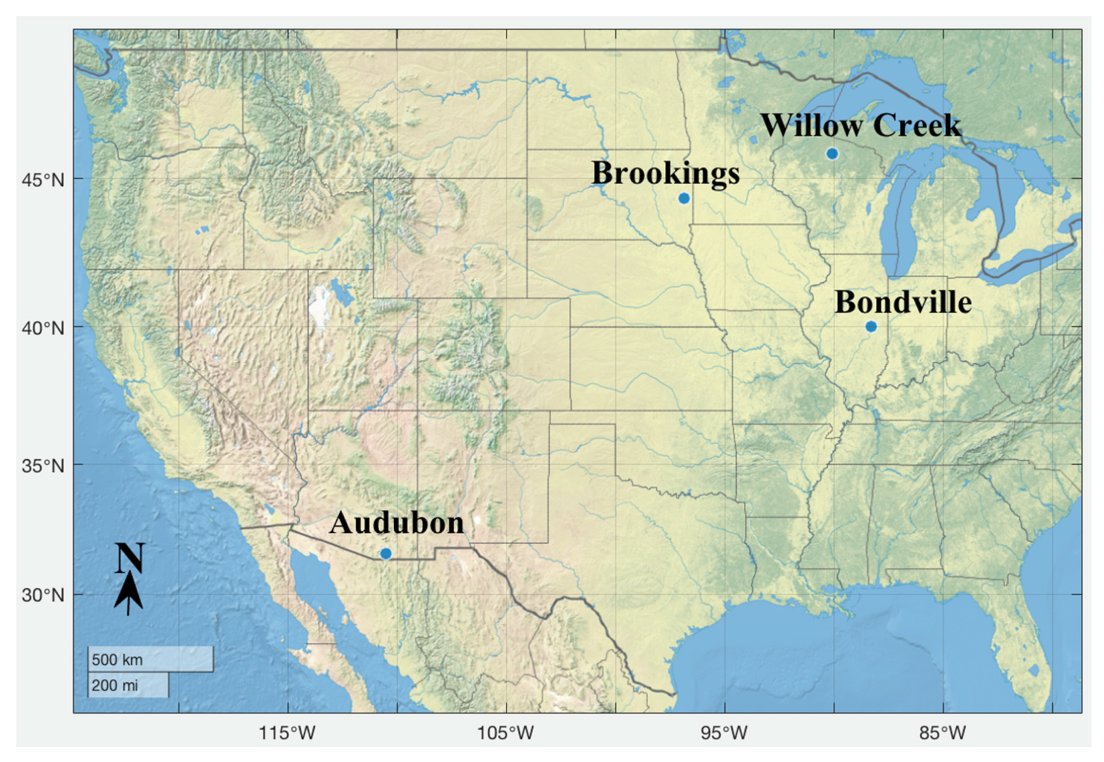
| Willow Creek, WI | 2005 | 170–259 | 45.8059°N | 90.0799°W | Forest | 0.22 | 5.67 | 520 |
| Brookings, SD | 2009 | 176–265 | 44.3453°N | 96.8362°W | Grassland | 0.29 | 1.72 | 510 |
| Bondville, IL | 2005 | 182–271 | 40.0062°N | 88.2904°W | Cropland | 0.16 | 2.24 | 219 |
| Audubon, AZ | 2006 | 170–259 | 31.5907°N | 110.5092°W | Grassland | 0.12 | 0.54 | 1469 |
| Desert, China | 2015 | 170–259 | 42.1100°N | 100. 9900°E | Barren land | 0.03 | 0 | 1000 |
| Site | (m) | (K) | (kg kg−1) | (K km−1) | (kg kg−1 km−1) |
|---|---|---|---|---|---|
| Arou | 400 | 4.5 | −2.9 10−3 | 5.7 | −1.2 10−3 |
| Willow Creek | 400 | 4.4 | −3.2 10−3 | 5.5 | −1.5 10−3 |
| Brookings | 400 | 4.0 | −2.0 10−3 | 4.5 | −0.5 10−3 |
| Bondville | 400 | 4.0 | −4.0 10−3 | 4.5 | −3.0 10−3 |
| Audubon | 400 | 2.8 | −4.4 10−3 | 3.0 | −4.0 10−3 |
| Desert | 400 | 2.4 | −4.4 10−3 | 3.0 | −4.5 10−3 |
| Site | DOY | CHN | LAI |
|---|---|---|---|
| Arou | 170–199 | 0.0102 | 2.97 |
| 200–229 | 0.0325 | 4.41 | |
| 230–259 | 0.0261 | 3.35 | |
| 170–199 | 0.0245 | 5.87 | |
| Willow Creek | 200–229 | 0.0242 | 5.84 |
| 230–259 | 0.0222 | 5.29 | |
| Brookings | 176–206 | 0.0054 | 1.93 |
| 207–237 | 0.0102 | 2.15 | |
| 238–265 | 0.0048 | 1.07 | |
| Bondville | 182–211 | 0.0130 | 2.23 |
| 212–241 | 0.0150 | 2.24 | |
| 242–271 | 0.0140 | 2.24 | |
| Audubon | 170–199 | 0.0031 | 0.27 |
| 200–229 | 0.0029 | 0.57 | |
| 230–259 | 0.0033 | 0.77 | |
| Desert | 170–199 | 0.0022 | 0 |
| 200–229 | 0.0020 | 0 | |
| 230–259 | 0.0010 | 0 |
| Site | EF | SM | LAI | |
|---|---|---|---|---|
| MAE | RMSE | |||
| Arou | 0.039 | 0.053 | 0.36 | 3.57 |
| Willow Creek | 0.067 | 0.079 | 0.22 | 5.67 |
| Brookings | 0.065 | 0.083 | 0.29 | 1.72 |
| Bondville | 0.073 | 0.091 | 0.16 | 2.24 |
| Audubon | 0.146 | 0.178 | 0.12 | 0.54 |
| Desert | 0.152 | 0.198 | 0.03 | 0.00 |
| Site | Method | H (Wm−2) | LE (Wm−2) | ||
|---|---|---|---|---|---|
| MAE | RMSE | MAE | RMSE | ||
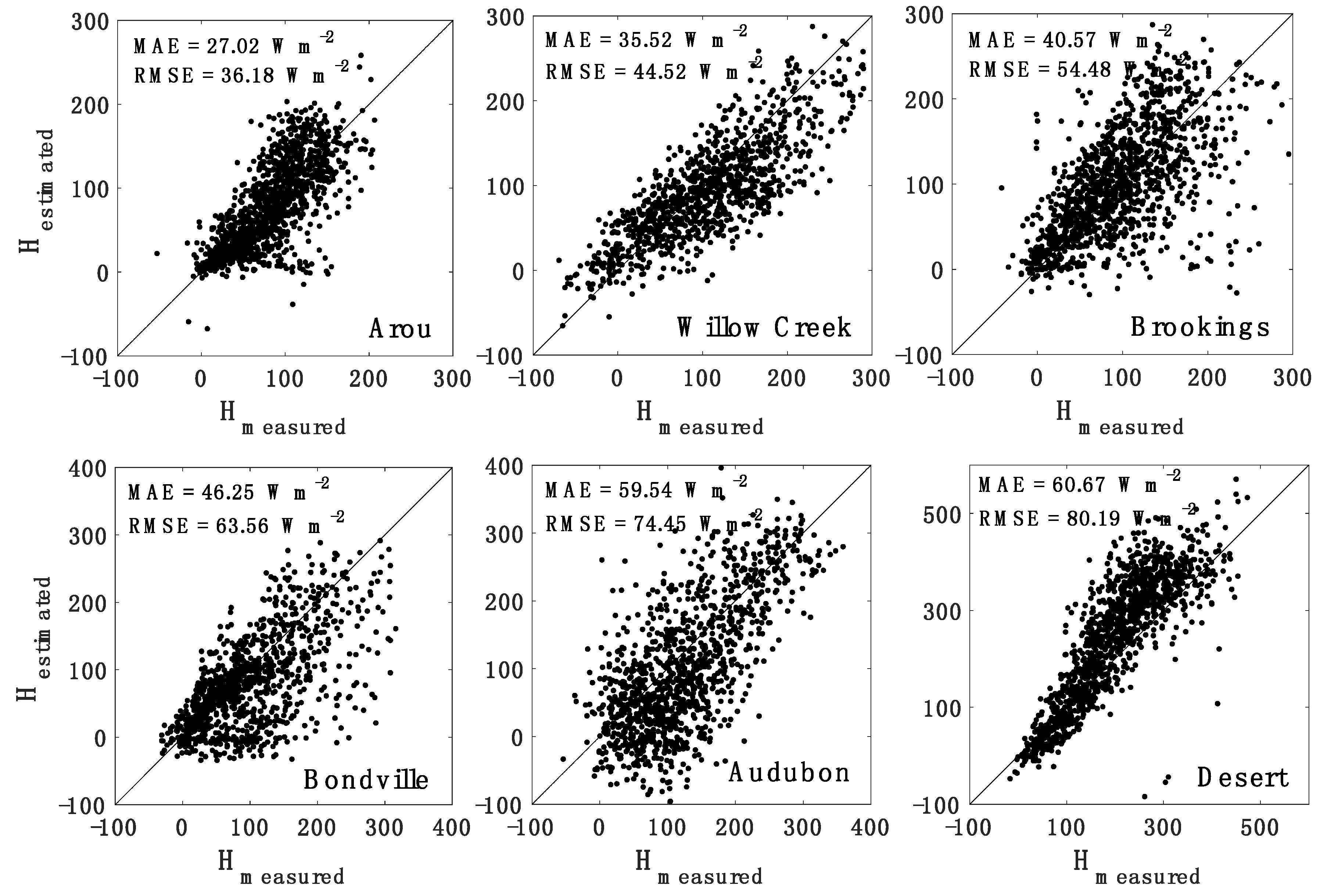
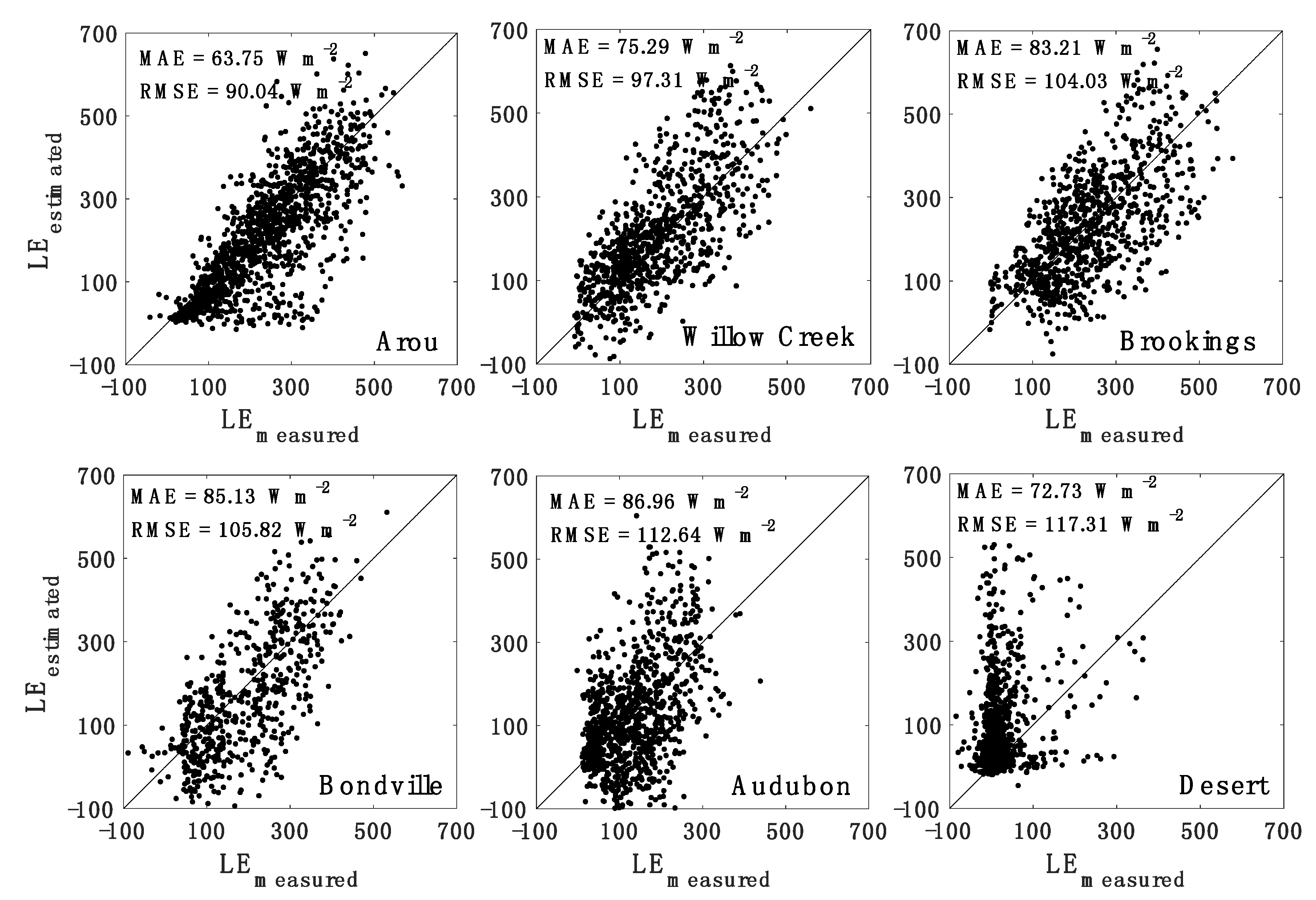
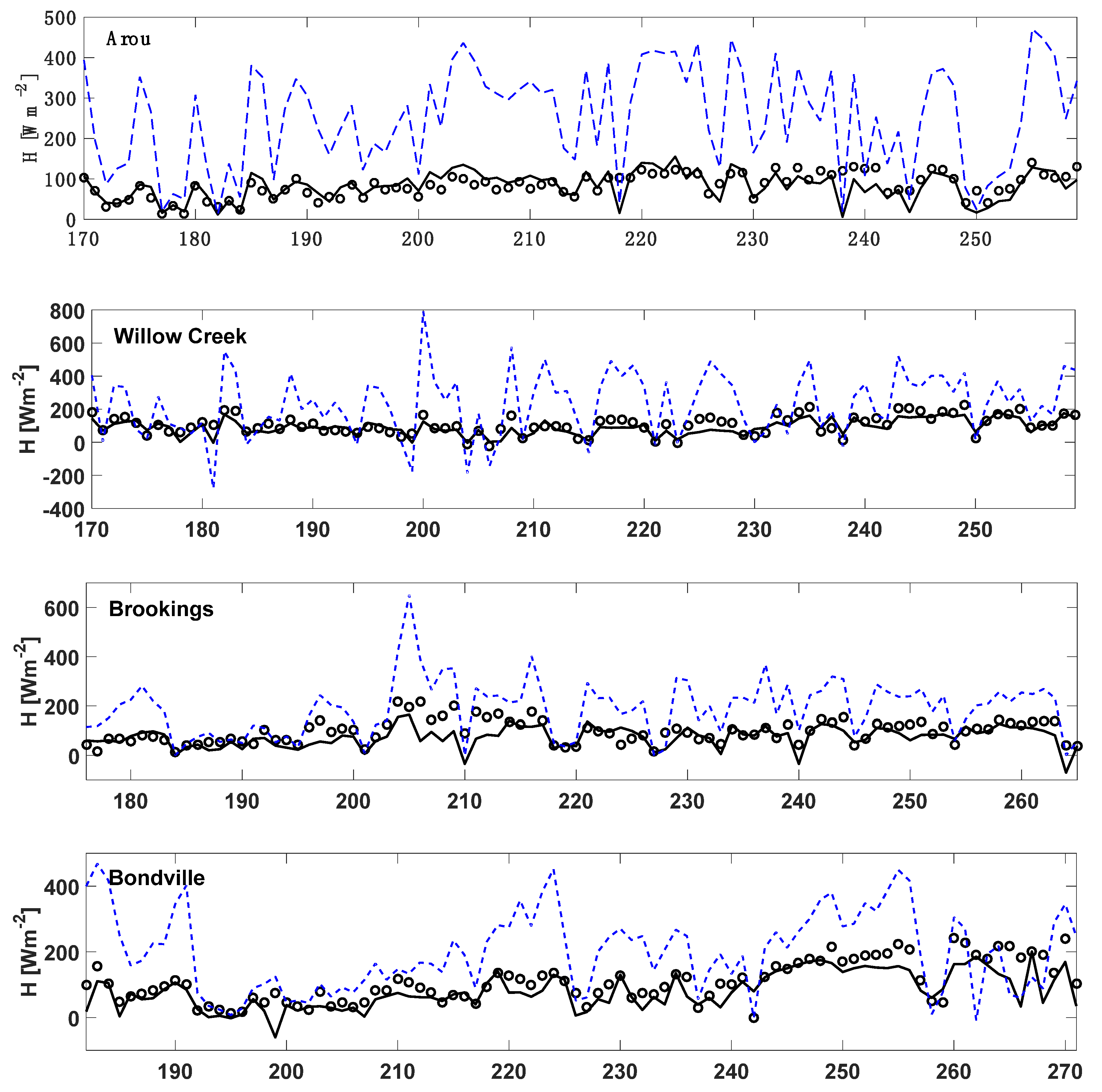
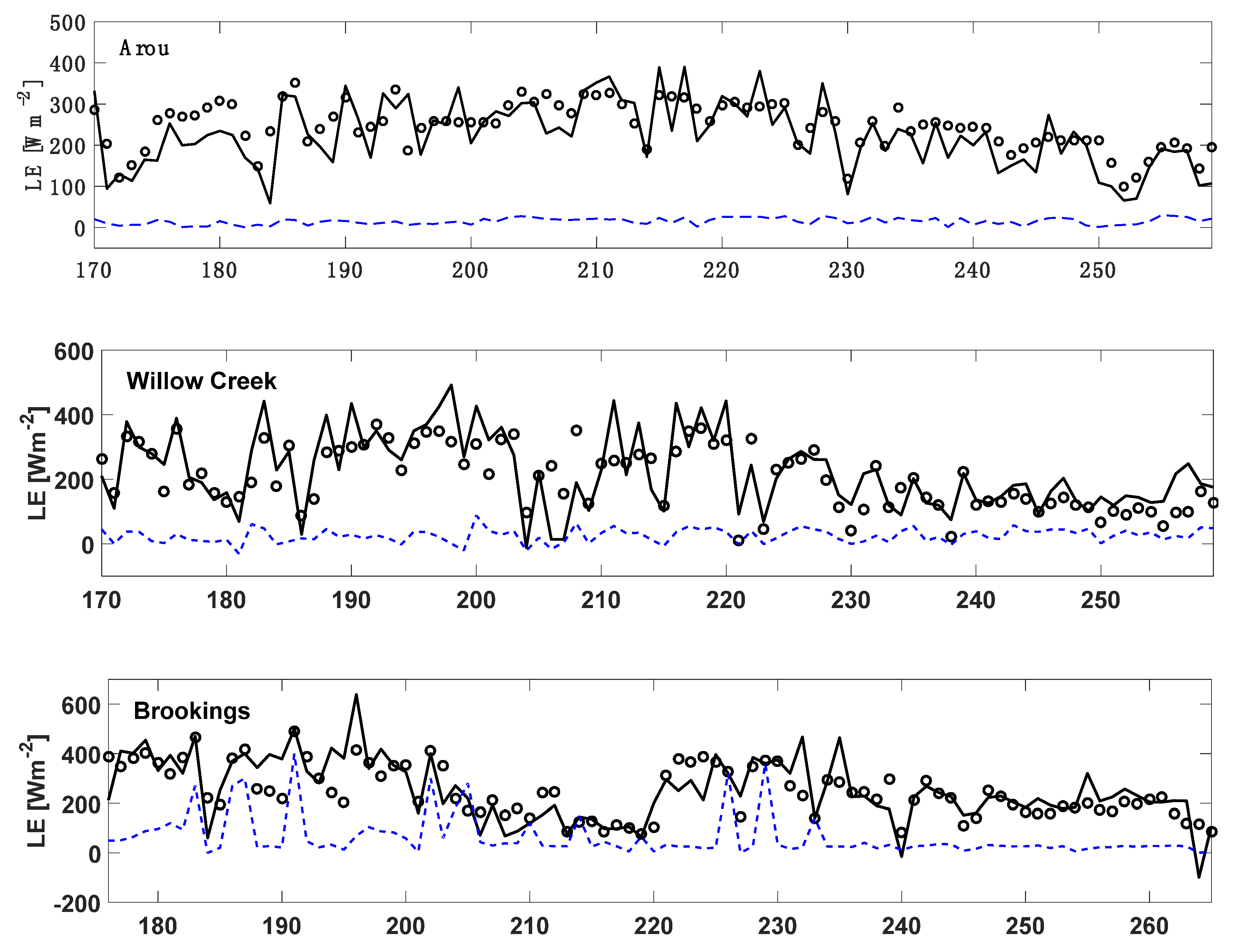
| Arou | VDA (Open-loop) | 27.02 (205.92) | 36.18 (242.09) | 63.75 (219.33) | 90.04 (247.15) |
| Willow Creek | VDA (Open-loop) | 35.52 (188.52) | 44.52 (223.67) | 75.29 (179.98) | 97.31 (239.42) |
| Brookings | VDA (Open-loop) | 40.57 (105.89) | 54.48 (138.58) | 83.21 (212.36) | 104.03 (239.00) |
| Bondville | VDA (Open-loop) | 46.25 (118.67) | 63.56 (158.02) | 85.13 (156.58) | 105.82 (188.92) |
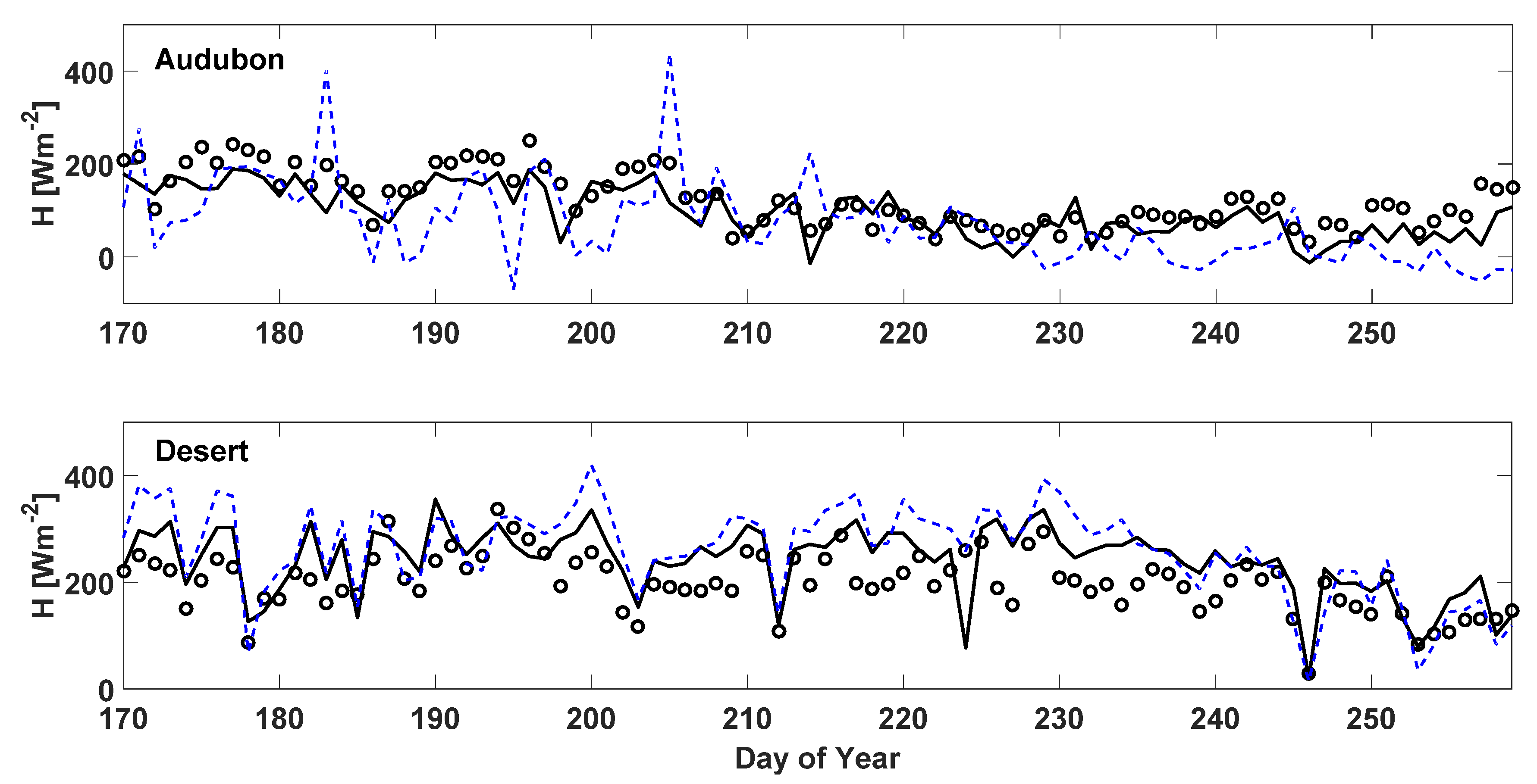
| Audubon | VDA (Open-loop) | 59.54 (107.75) | 74.45 (127.97) | 86.96 (140.09) | 112.64 (166.11) |
| Desert | VDA (Open-loop) | 60.67 (77.78) | 80.19 (103.76) | 72.73 (95.96) | 117.31 (156.28) |
| Six-site average | VDA (Open-loop) | 44.93 (134.09) | 58.89 (165.68) | 77.85 (167.38) | 104.53 (206.15) |
| Site | Method | H (Wm−2) | LE (Wm−2) | ||
|---|---|---|---|---|---|
| MAE | RMSE | MAE | RMSE | ||
| Arou | VDA (Open-loop) | 18.07 (172.66) | 25.43 (197.61) | 43.99 (231.71) | 55.81 (237.78) |
| Willow Creek | VDA (Open-loop) | 30.05 (157.65) | 37.03 (197.65) | 56.93 (179.33) | 74.46 (200.28) |
| Brookings | VDA (Open-loop) | 32.05 (100.47) | 45.01 (123.03) | 57.79 (185.88) | 82.28 (207.54) |
| Bondville | VDA (Open-loop) | 31.97 (108.15) | 45.21 (134.12) | 55.34 (152.44) | 77.88 (172.74) |
| Audubon | VDA (Open-loop) | 46.16 (74.73) | 58.13 (91.77) | 71.77 (125.67) | 89.57 (145.45) |
| Desert | VDA (Open-loop) | 50.08 (67.07) | 60.00 (80.95) | 68.74 (90.23) | 102.21 (132.62) |
| Six-site average | VDA (Open-loop) | 34.73 (113.46) | 45.14 (137.52) | 59.09 (160.88) | 80.37 (182.74) |
© 2020 by the authors. Licensee MDPI, Basel, Switzerland. This article is an open access article distributed under the terms and conditions of the Creative Commons Attribution (CC BY) license (http://creativecommons.org/licenses/by/4.0/).
Share and Cite
Tajfar, E.; Bateni, S.M.; Heggy, E.; Xu, T. Feasibility of Estimating Turbulent Heat Fluxes via Variational Assimilation of Reference-Level Air Temperature and Specific Humidity Observations. Remote Sens. 2020, 12, 1065. https://doi.org/10.3390/rs12071065
Tajfar E, Bateni SM, Heggy E, Xu T. Feasibility of Estimating Turbulent Heat Fluxes via Variational Assimilation of Reference-Level Air Temperature and Specific Humidity Observations. Remote Sensing. 2020; 12(7):1065. https://doi.org/10.3390/rs12071065
Chicago/Turabian StyleTajfar, Elahe, Sayed M. Bateni, Essam Heggy, and Tongren Xu. 2020. "Feasibility of Estimating Turbulent Heat Fluxes via Variational Assimilation of Reference-Level Air Temperature and Specific Humidity Observations" Remote Sensing 12, no. 7: 1065. https://doi.org/10.3390/rs12071065