Potential Instability of Gas Hydrates along the Chilean Margin Due to Ocean Warming

 , ,
, ,  , and
, and
Abstract
:1. Introduction
2. Materials and Methods
2.1. Data Collection and Analysis
2.2. Modelling
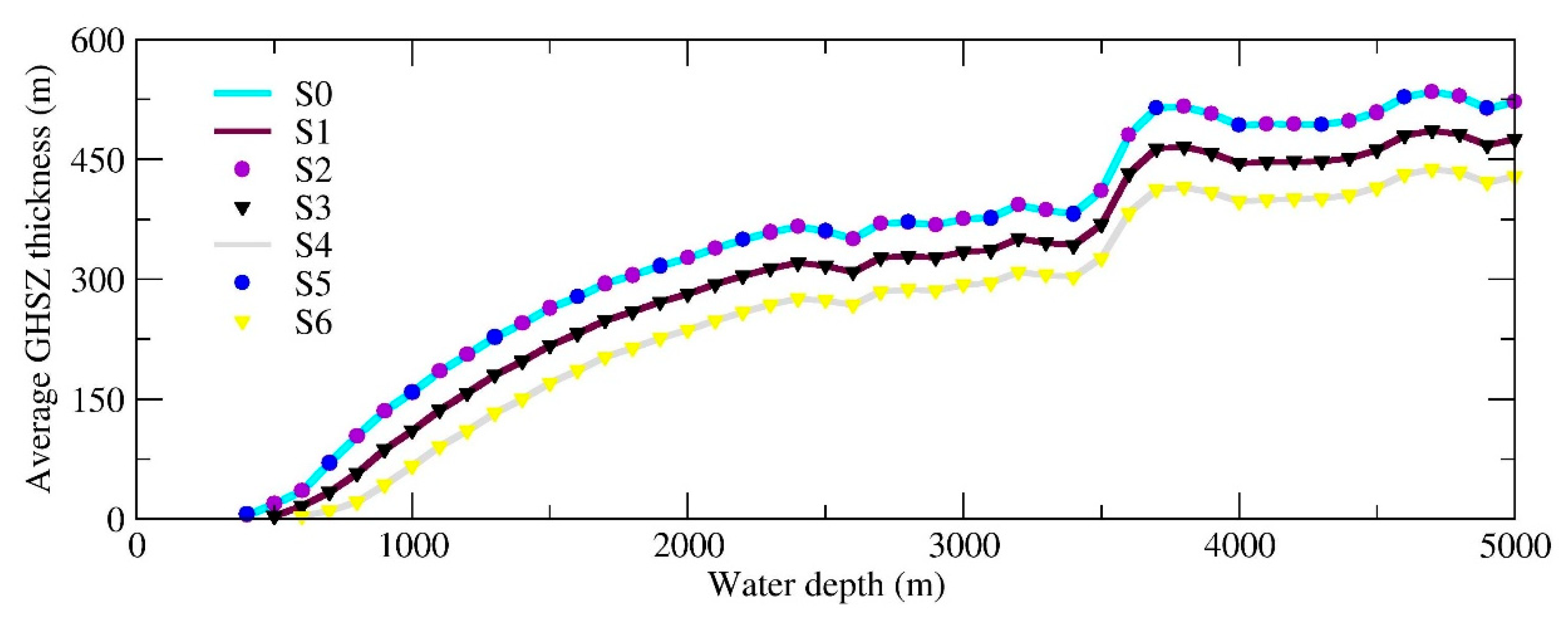
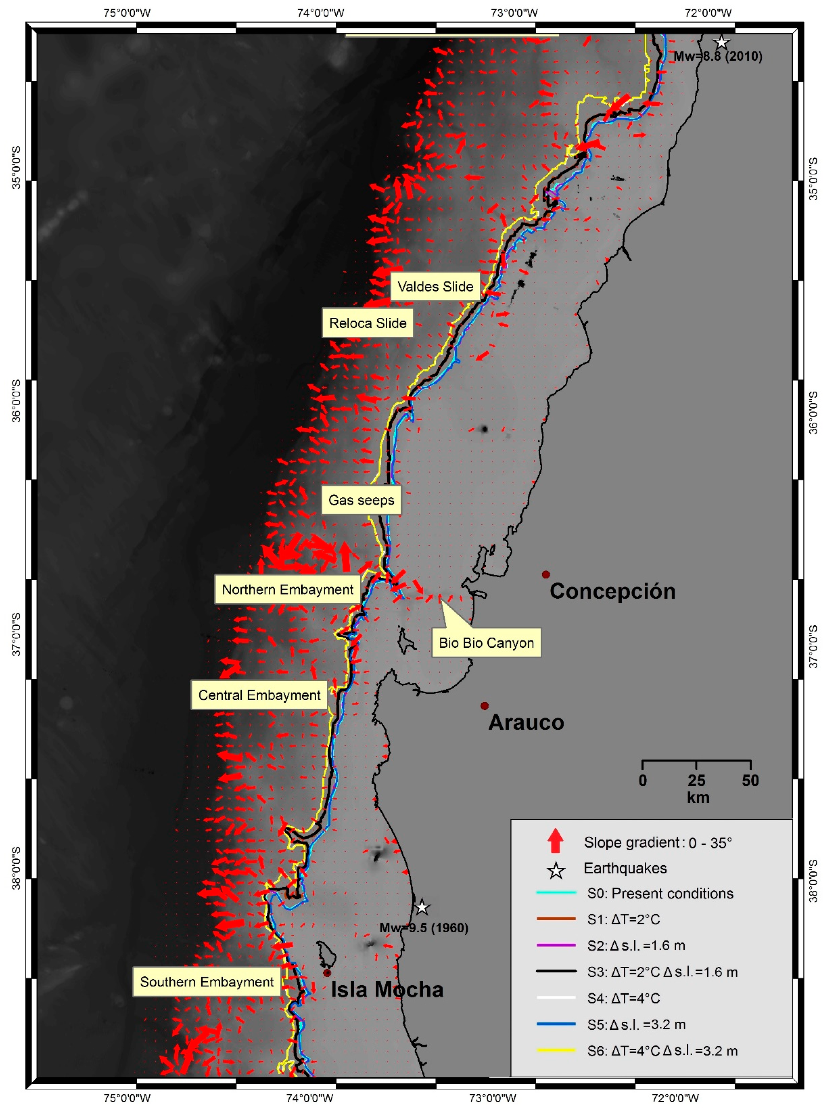
3. Results
4. Discussion
5. Conclusions
Author Contributions
Funding
Acknowledgments
Conflicts of Interest
References
- Makogon, Y.F. Hydrate of Hydrocarbons; PennWell Publishing Co.: Tulsa, Oklahoma, 1997. [Google Scholar]
- Moridis, G.J.; Collett, T.S.; Boswell, R.; Kurihara, M.; Reagan, M.T.; Koh, C.; Sloan, E.D. Toward production from gas hydrates: Current status, assessment of resources, and simulation-based evaluation of technology and potential. SPE Reserv. Eval. Eng. 2009, 12, 745–771. [Google Scholar] [CrossRef]
- Sloan, E.D., Jr. Clathrate Hydrates of Natural Gases, 2nd ed.; Revised and Expanded; Marcel Dekker, Inc.: New York, NY, USA, 1998; p. 705. [Google Scholar]
- Marín-Moreno, H.; Giustiniani, M.; Tinivella, U. The potential response of the hydrate reservoir in the South Shetland Margin, Antarctic Peninsula, to ocean warming over the 21st century. Polar Res. 2015, 34, 27443. [Google Scholar] [CrossRef]
- IPCC. Contribution of Working Groups I, II and III to the Fifth Assessment Report of the Intergovernmental Panel on Climate Change. In Climate Change 2014: Synthesis Report; Pachauri, R.K., Meyer, L.A., Eds.; IPCC: Geneva, Switzerland, 2014; 151p. [Google Scholar]
- Wallman, K.; MIGRATE Consortium. Marine Gas Hydrate—An Indigenous Resource of Natural Gas for Europe (MIGRATE). 2015; Available online: https://www.migrate-cost.eu/ (accessed on 29 April 2019).
- MacDonald, I.; Joye, S. Lair of the “Ice Worm”. Quarterdeck 1997, 5, 5–7. [Google Scholar]
- Kvenvolden, K.A. Methane hydrate in the global organic carbon cycle. Terra Nova 2002, 14, 302–306. [Google Scholar] [CrossRef]
- Kennett, J.P.; Cannariato, K.G.; Hendy, I.L.; Behl, R.J. Role of Methane Hydrates in Late Quaternary Climatic Change: The Clathrate Gun Hypothesis; AGU: Washington, DC, USA, 2003; Volume 54, 216p. [Google Scholar]
- Dickens, G.R. Modeling the global carbon cycle with a gas hydrate capacitor: Significance for the latest Paleocene thermal maximum. In Natural Gas Hydrates: Occurrence, Distribution, and Detection; Paull, C.K., Dillon, W.P., Eds.; Geophysical Monograph Series; American Geophysical Union: Washington, DC, USA, 2001; Volume 124, pp. 19–40. [Google Scholar]
- Xu, W.; Lowell, R.P.; Peltzer, E.T. Effect of seafloor temperature and pressure variations on methane flux from a gas hydrate layer: Comparison between current and late Paleocene climate conditions. J. Geophys. Res. Solid Earth 2001, 106, 26413–26423. [Google Scholar] [CrossRef] [Green Version]
- Milkov, A.V. Global estimates of hydrate-bound gas in marine sediments: How much is really out there? Earth-Sci. Rev. 2004, 66, 183–197. [Google Scholar] [CrossRef]
- Vargas-Cordero, I.; Tinivella, U.; Villar-Muñoz, L.; Bento, J. High Gas Hydrate and Free Gas Concentrations: An Explanation for Seeps Offshore South Mocha Island. Energies 2018, 11, 3062. [Google Scholar] [CrossRef]
- Kvenvolden, K.A. Potential effects of gas hydrate on human welfare. Proc. Natl. Acad. Sci. USA 1999, 96, 3420–3426. [Google Scholar] [CrossRef] [Green Version]
- Sultan, N.; Cochonat, P.; Foucher, J.P.; Mienert, J. Effect of gas hydrates melting on seafloor slope instability. Mar. Geol. 2004, 213, 379–401. [Google Scholar] [CrossRef] [Green Version]
- Sultan, N.; Cochonat, P.; Canals, M.; Cattaneo, A.; Dennielou, B.; Haflidason, H.; Laberg, J.S.; Long, D.; Mienert, J.; Trincardi, F.; et al. Triggering mechanisms of slope instability processes and sediment failures on continental margins: A geotechnical approach. Mar. Geol. 2004, 213, 291–321. [Google Scholar] [CrossRef]
- Tinivella, U. The seismic response to over-pressure versus gas hydrate and free gas concentration. J. Seism. Explor. 2002, 11, 283–305. [Google Scholar]
- Tinivella, U.; Giustiniani, M.; Accettella, D. 2011. BSR versus climate change and slides. J. Geol. Res. 2011, 2011, 390547. [Google Scholar]
- Boobalan, A.J.; Ramanujam, N. Triggering mechanism of gas hydrate dissociation and subsequent sub marine landslide and ocean wide Tsunami after Great Sumatra—Andaman 2004 earthquake. Arch. Appl. Sci. Res. 2013, 5, 105–110. [Google Scholar]
- Bangs, N.L.; Sawyer, D.S.; Golovchenko, X. Free gas at the base of the gas hydrate zone in the vicinity of the Chile triple junction. Geology 1993, 21, 905–908. [Google Scholar] [CrossRef]
- Rodrigo, C.; González-Fernández, A.; Vera, E. Variability of the bottom-simulating reflector (BSR) and its association with tectonic structures in the Chilean margin between Arauco Gulf (37° S) and Valdivia (40° S). Mar. Geophys. Res. 2009, 30, 1–19. [Google Scholar] [CrossRef]
- Vargas-Cordero, I.; Tinivella, U.; Accaino, F.; Loreto, M.F.; Fanucci, F.; Reichert, C. Analyses of bottom simulating reflections offshore Arauco and Coyhaique (Chile). Geo-Mar. Lett. 2010, 30, 271–281. [Google Scholar] [CrossRef]
- Cande, S.C.; Leslie, R.B.; Parra, J.C.; Hobart, M. Interaction between the Chile Ridge and Chile Trench: Geophysical and geothermal evidence. J. Geophys. Res: Solid Earth 1987, 92, 495–520. [Google Scholar] [CrossRef]
- Froelich, P.N.; Kvenvolden, K.A.; Torres, M.E.; Waseda, A.; Didyk, B.M.; Lorenson, T.D. Geochemical evidence for gas hydrate in sediment near the Chile Triple Junction. Proc. ODP Sci. Results 1995, 141, 279–287. [Google Scholar]
- Sloan, E.D., Jr.; Koh, C. Clathrate Hydrates of Natural Gases, 3rd ed.; CRC Press: Boca Raton, FL, USA, 2007; p. 752. [Google Scholar]
- Vargas-Cordero, I.; Tinivella, U.; Accaino, F.; Fanucci, F.; Loreto, M.F.; Lascano, M.E.; Reichert, C. Basal and frontal accretion processes versus BSR characteristics along the Chilean margin. J. Geol. Res. 2011, 2011, 846101. [Google Scholar] [CrossRef]
- Vargas-Cordero, I.; Tinivella, U.; Villar-Muñoz, L.; Giustiniani, M. Gas hydrate and free gas estimation from seismic analysis offshore Chiloé island (Chile). Andean Geol. 2016, 43, 263–274. [Google Scholar] [CrossRef]
- Vargas-Cordero, I.; Tinivella, U.; Villar-Muñoz, L. Gas Hydrate and Free Gas Concentrations in Two Sites inside the Chilean Margin (Itata and Valdivia Offshores). Energies 2017, 10, 2154. [Google Scholar] [Green Version]
- Grevemeyer, I.; Villinger, H. Gas hydrate stability and the assessment of heat flow through continental margins. Geophys. J. Int. 2001, 145, 647–660. [Google Scholar] [CrossRef] [Green Version]
- Vargas-Cordero, I.; Tinivella, U.; Accaino, F.; Loreto, M.F.; Fanucci, F. Thermal state and concentration of gas hydrate and free gas of Coyhaique, Chilean Margin (44 30′ S). Mar. Pet. Geol. 2010, 27, 1148–1156. [Google Scholar] [CrossRef]
- Villar-Muñoz, L.; Bento, J.P.; Klaeschen, D.; Tinivella, U.; Vargas-Cordero, I.; Behrmann, J.H. A first estimation of gas hydrates offshore Patagonia (Chile). Mar. Pet. Geol. 2018, 96, 232–239. [Google Scholar] [CrossRef]
- Bangs, N.L.; Cande, S.C. Episodic development of a convergent margin inferred from structures and processes along the southern Chile margin. Tectonics 1997, 16, 489–503. [Google Scholar] [CrossRef]
- Ramos, V. Plate tectonic setting of the Andean Cordillera. Episodes 1999, 22, 183–190. [Google Scholar] [Green Version]
- Grevemeyer, I.; Diaz-Naveas, J.L.; Ranero, C.R.; Villinger, H.W. Heat flow over the descending Nazca plate in central Chile, 32 S to 41 S: Observations from ODP Leg 202 and the occurrence of natural gas hydrates. Earth Planet. Sci. Lett. 2003, 213, 285–298. [Google Scholar] [CrossRef]
- Melnick, D. Neogene Seismotectonics of the South-Central Chile Margin: Subduction-Related Processes over Various Temporal and Spatial Scales. Ph.D. Thesis, Universität Potsdam, Potsdam, Germany, 2007. [Google Scholar]
- Cembrano, J.; Lara, L. The link between volcanism and tectonics in the southern volcanic zone of the Chilean Andes: A review. Tectonophysics 2009, 471, 96–113. [Google Scholar] [CrossRef]
- Vargas-Cordero, I. Gas Hydrate Occurrence and Morpho-Structures along Chilean Margin. Ph.D. Dissertation, Fisiche e Naturali, Università di Trieste, Trieste, Italy, 2009. [Google Scholar]
- Manea, V.C.; Pérez-Gussinyé, M.; Manea, M. Chilean flat slab subduction controlled by overriding plate thickness and trench rollback. Geology 2012, 40, 35–38. [Google Scholar] [CrossRef]
- Melnick, D.; Echtler, H.P. Inversion of forearc basins in south-central Chile caused by rapid glacial age trench fill. Geology 2006, 34, 709–712. [Google Scholar] [CrossRef]
- Maksymowicz, A. The geometry of the Chilean continental wedge: Tectonic segmentation of subduction processes off Chile. Tectonophysics 2015, 659, 183–196. [Google Scholar] [CrossRef]
- GMRTMapTool. Available online: https://www.gmrt.org/GMRTMapTool/ (accessed on 29 April 2019).
- National Oceanographic Data Center (NODC). Available online: https://www.nodc.noaa.gov/OC5/woa13/woa13data.html (accessed on 29 April 2019).
- Bangs, N.L.; Brown, K.M. Regional heat flow in the vicinity of the Chile Triple Junction constrained by the depth of the bottom simulating reflection. Proc. ODP Sci. Results 1995, 141, 253–259. [Google Scholar]
- Villar-Muñoz, L.; Behrmann, J.H.; Diaz-Naveas, J.; Klaeschen, D.; Karstens, J. Heat flow in the southern Chile forearc controlled by large-scale tectonic processes. Geo-Mar. Lett. 2014, 34, 185–198. [Google Scholar]
- Mix, A.C.; Tiedemann, R.; Blum, P. Shipboard Scientific Party Proceedings of the ODP; Initial Reports; Ocean Drilling Program: College Station, TX, USA, 2003; pp. 1–145. [Google Scholar]
- Tinivella, U.; Giustiniani, M. Variations in BSR depth due to gas hydrate stability versus pore pressure. Glob. Planet. Chang. 2013, 100, 119–128. [Google Scholar] [CrossRef]
- Khan, M.J.; Ali, M. A Review of Research on Gas Hydrates in Makran. Bahria Univ. Res. J. Earth Sci. 2016, 1, 28–35. [Google Scholar]
- Dickens, G.R.; Quinby-Hunt, M.S. Methane hydrate stability in pore water: A simple theoretical approach for geophysical applications. J. Geophys. Res. 1997, 102, 773–783. [Google Scholar] [CrossRef]
- NASA Global Climate Change. Available online: https://climate.nasa.gov/scientific-consensus/ (accessed on 29 April 2019).
- Coffin, R.; Pohlman, J.; Gardner, J.; Downer, R.; Wood, W.; Hamdan, L.; Walker, S.; Plummer, R.; Gettrust, J.; Diaz, J. Methane hydrate exploration on the mid Chilean coast: A geochemical and geophysical survey. J. Pet. Sci. Eng. 2007, 56, 32–41. [Google Scholar] [CrossRef]
- Marín-Moreno, H.; Giustiniani, M.; Tinivella, U.; Piñero, E. The challenges of quantifying the carbon stored in Arctic marine gas hydrate. Mar. Pet. Geol. 2016, 71, 76–82. [Google Scholar] [CrossRef] [Green Version]
- Thatcher, K.E.; Westbrook, G.K.; Sarkar, S.; Minshull, T.A. Methane release from warming-induced hydrate dissociation in the West Svalbard continental margin: Timing, rates, and geological controls. J. Geophys. Res. Solid Earth 2013, 118, 22–38. [Google Scholar] [CrossRef]
- Ruppel, C.D.; Kessler, J.D. The interaction of climate change and methane hydrates. Rev. Geophys. 2017, 55, 126–168. [Google Scholar] [CrossRef]
- Contreras-Reyes, E.; Völker, D.; Bialas, J.; Moscoso, E.; Grevemeyer, I. Reloca Slide: An ~24 km3 submarine mass-wasting event in response to over-steepening and failure of the central Chilean continental slope. Terra Nova 2016, 28, 257–264. [Google Scholar] [CrossRef]
- Geersen, J.; Völker, D.; Behrmann, J.H.; Reichert, C.; Krastel, S. Pleistocene giant slope failures offshore Arauco peninsula, southern Chile. J. Geol. Soc. 2011, 168, 1237–1248. [Google Scholar] [CrossRef]
- Völker, D.; Geersen, J.; Behrmann, J.H.; Weinrebe, W.R. Submarine mass wasting off Southern Central Chile: Distribution and possible mechanisms of slope failure at an active continental margin. In Submarine Mass Movements and their Consequences. Advances in Natural and Technological Hazards Research; Yamada, Y., Kawamura, K., Ikehara, K., Ogawa, Y., Urgeles, R., Mosher, D., Chaytor, J., Strasser, M., et al., Eds.; Springer: Dordrecht, The Netherlands, 2012; pp. 379–389. [Google Scholar]
- Geersen, J.; Völker, D.; Behrmann, J.H.; Kläschen, D.; Weinrebe, W.; Krastel, S.; Reichert, C. Seismic rupture during the 1960 Great Chile and the 2010 Maule earthquakes limited by a giant Pleistocene submarine slope failure. Terra Nova 2013, 25, 472–477. [Google Scholar] [CrossRef]
- Klaucke, I.; Weinrebe, W.; Linke, P.; Kläschen, D.; Bialas, J. Sidescan sonar imagery of widespread fossil and active cold seeps along the central Chilean continental margin. Geo-Mar. Lett. 2012, 32, 489–499. [Google Scholar] [CrossRef]
- USGS Science for a Changing World. Available online: https://earthquake.usgs.gov/earthquakes/ (accessed on 29 April 2019).
- Sawyer, D.E.; DeVore, J.R. Elevated shear strength of sediments on active margins: Evidence for seismic strengthening. Geophys. Res. Lett. 2015, 42, 10–216. [Google Scholar] [CrossRef]
- Brothers, D.S.; Andrews, B.D.; Walton, M.A.; Greene, H.G.; Barrie, J.V.; Miller, N.C.; Brink, U.T.; East, A.E.; Haeussler, P.J.; Kluesner, J.W.; et al. Slope failure and mass transport processes along the Queen Charlotte Fault, southeastern Alaska. In Subaqueous Mass Movements; Lintern, D.G., Mosher, D.C., Moscardelli, L.G., Bobrowsky, P.T., Campbell, C., Chaytor, J.D., Clague, J.J., Georgiopoulou, A., Lajeunesse, P., Normandeau, A., Eds.; Geological Society: London, UK, 2018; p. SP477-30. [Google Scholar]
- Greene, H.G.; Barrie, J.V.; Brothers, D.S.; Conrad, J.E.; Conway, K.; East, A.E.; Enkin, R.; Maier, K.L.; Nishenko, S.P.; Walton, M.A.; et al. Slope failure and mass transport processes along the Queen Charlotte Fault Zone, western British Columbia. In Subaqueous Mass Movements; Lintern, D.G., Mosher, D.C., Moscardelli, L.G., Bobrowsky, P.T., Campbell, C., Chaytor, J.D., Clague, J.J., Georgiopoulou, A., Lajeunesse, P., Normandeau, A., Eds.; Geological Society: London, UK, 2018; p. SP477-30. [Google Scholar]
- Sawyer, D.E.; Reece, R.S.; Gulick, S.P.; Lenz, B.L. Submarine landslide and tsunami hazards offshore southern Alaska: Seismic strengthening versus rapid sedimentation. Geophys. Res. Lett. 2017, 44, 8435–8442. [Google Scholar] [CrossRef]
- Giustiniani, M.; Tinivella, U.; Jakobsson, M.; Rebesco, M. Arctic Ocean gas hydrate stability in a changing climate. J. Geol. Res. 2013, 2013, 783969. [Google Scholar] [CrossRef]
- Gorman, A.R.; Senger, K. Defining the updip extent of the gas hydrate stability zone on continental margins with low geothermal gradients. J. Geophys. Res. Solid Earth 2010, 115, B07105. [Google Scholar] [CrossRef]


| Scenario | Gas Hydrate Dissociation Area | Total Volume | Pore Volume | Hydrate Volume | Gas Volume |
|---|---|---|---|---|---|
| S1 (ΔT = 2 °C) | 3% | 113 km3 | 45 km3 | 1.36 km3 | 222 km3 |
| S4 (ΔT = 4 °C) | 6.5% | 482 km3 | 193 km3 | 5.79 km3 | 950 km3 |
© 2019 by the authors. Licensee MDPI, Basel, Switzerland. This article is an open access article distributed under the terms and conditions of the Creative Commons Attribution (CC BY) license (http://creativecommons.org/licenses/by/4.0/).
Share and Cite
Alessandrini, G.; Tinivella, U.; Giustiniani, M.; de la Cruz Vargas-Cordero, I.; Castellaro, S. Potential Instability of Gas Hydrates along the Chilean Margin Due to Ocean Warming. Geosciences 2019, 9, 234. https://doi.org/10.3390/geosciences9050234
Alessandrini G, Tinivella U, Giustiniani M, de la Cruz Vargas-Cordero I, Castellaro S. Potential Instability of Gas Hydrates along the Chilean Margin Due to Ocean Warming. Geosciences. 2019; 9(5):234. https://doi.org/10.3390/geosciences9050234
Chicago/Turabian StyleAlessandrini, Giulia, Umberta Tinivella, Michela Giustiniani, Iván de la Cruz Vargas-Cordero, and Silvia Castellaro. 2019. "Potential Instability of Gas Hydrates along the Chilean Margin Due to Ocean Warming" Geosciences 9, no. 5: 234. https://doi.org/10.3390/geosciences9050234