A Study on Neutral-Point Potential in Three-Level NPC Converters

Abstract

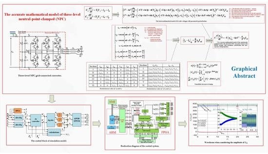
This paper proposes an accurate mathematical model of three-level neutral-point-clamped (NPC) converters that can accurately represent the midpoint potential drift of the DC link with parameter perturbation. The mathematical relationships between the fluctuation in neutral-point voltage, the parametric perturbation, and the capacitance error are obtained as mathematical expressions in this model. The expressions can be used to quantitatively analyze the reason for the neutral-point voltage imbalance and balancing effect based on a zero-sequence voltage injection. The injected zero-sequence voltage, which can be used to balance the DC-side voltages with the combined action of active current, can be easily obtained from the proposed model. A balancing control under four-quadrant operation modes is proposed by considering the active current to verify the effectiveness of this model. Both the simulation and experiment results validate the excellent performance of the proposed model compared to the conventional model.

1. Introduction

Three-level neutral-point-clamped (NPC) converters are popularly used in renewable energy generation and energy storage, which have been widely recognized as promising solutions to the problems associated with increasing environmental challenges [1,2,3]. Compared to the two-level topology, three-level NPC converters are much more attractive because of their lower voltage stress on power electronic devices, lower total harmonic distortion, higher efficiency, and even better economic performance [4,5,6].

However, the neutral-point potential drift, which results in an imbalance of voltages of the two DC-side capacitors, is an inherent problem for the three-level NPC topology. Without considering the sampling error, capacitance error, inconsistent characteristics of devices, and operation under unbalanced conditions are usually considered the reasons for potential drift. How to keep the upper and lower voltages equal is very important for the devices to run safely and reliably [7,8,9].

Numerous research works have been carried out to realize control of the DC-side voltage balance [10,11,12,13,14,15,16,17,18,19,20,21,22,23,24,25,26,27]. In [14,15,16,17], it is proposed that the neutral-point potential of the inverters can be balanced by hardware, including independent DC voltage sources and auxiliary converters that inject current into the neutral point. But this method needs an additional circuit, which increases the cost, volume of the converter, and reduces the efficiency. In [18,19,20,21,22], several improved space vector pulse width modulation (SVPWM) strategies were proposed to adjust the dwell time between small vector switching states by judging the direction of the neutral point current and the deviation of the neutral point potential. However, the calculation methods are complex and difficult to implement. In [24], a pulse width modulation (PWM) strategy was proposed where the both DC-side voltages can be adjusted independently through zero-sequence voltage injections and compensation for the unbalance in neutral point voltages, but the process of calculating the injected zero-sequence voltages is complicated.

However, these control strategies, above all, ignore the quantitative analysis of the potential drift and balancing effect based on zero-sequence voltage injection. Meanwhile, if the converter is used in renewable energy generation and energy storage with four-quadrant operation modes, the DC voltage balancing control is very difficult to realize in existing literature because the active current of the converter is not taken into consideration.

This paper proposes an accurate mathematical model of the neutral-point potential in three-level NPC converters based on the SPWM strategy with parametric perturbation and zero-sequence voltage injection. The model is simple and direct, but very interesting and valuable. To the best of our knowledge, it is novel and has not been previously reported in the literature. From this model, the relationship between the drift potential value and all the AC-side and DC-side variables can be deduced by quantitative analyses. The calculated drift potential value shows that the basic reason for the neutral-point potential drift is the uneven shunt loss caused by the parametric perturbation, and the capacitance error has no influence on it. The balancing control can be directly obtained based on the combined action of the injected zero-sequence voltage and active current. The required zero-sequence voltage for balancing control can be easily calculated by this model.

The rest of this paper is organized as follows. Section 2 describes the main circuit topology, modulation strategy and AC-side current control. Section 3 develops the accurate mathematical model of the neutral-point potential drift, which shows the reason for the neutral-point potential drift. DC voltage control is realized in Section 4. In Section 5, the effectiveness and performance of this model and control strategy are verified by simulation and experiment.

2. Operation and Principles

2.1. Main Circuit Topology

The circuit topology of three-level NPC grid-connected converters used in renewable, energy-based applications is presented in Figure 1. The converter transfers active power from wind energy, photovoltaic energy, chemical energy, or the energy storage system to the distribution network. In some cases, it also can transfer active power from the distribution network to the energy storage system as well as compensate reactive power to the network.

As shown in Figure 1, U_dc denotes the DC-side voltage source, and Y_d is the internal resistor. u_x (x = a, b, c) is the system voltage, v_x is the output voltage of the converter. C₁ and C₂ are the two DC-side capacitors. Y₁ and Y₂ represent the shunt loss, including losses in the two parallel resistors and the power electronic switches. U₁ and U₂ are the two DC-side capacitor voltages. L_s is the linked reactor. The series losses are represented by the equivalent resistance R_s.

The purpose of DC-side voltage control is to maintain U₁ and U₂ at an equal and prespecified level.

2.2. Modulation Strategy

Power electronic switches in Figure 1 can be turned on and off based on the alternative phase opposition disposition (APOD) sine pulse width modulation (SPWM) strategy, as shown in Figure 2. Take phase a of Figure 1 as an example, s_a is the modulation signal with zero-sequence DC component s₀. CA₁ and CA₂ are the two triangular carrier waveforms with the same frequency, same amplitude, and contrary phases. Switches Q₁ and Q₃ are turned on and off based on the comparison of s_a and CA₁. Switches Q₂ and Q₄ are turned on and off based on the comparison of s_a and CA₂. Diodes D₁ and D₂ provide the bidirectional current path for the AC-side terminal to the common point of the DC capacitors O, when both Q₂ and Q₃ are on or off. Therefore, v_a swings between the neutral-point potential (here referred to as zero) when both Q₂ and Q₃ are on or off, U₁ when both Q₁ and Q₂ are on, and −U₂ when both Q₃ and Q₄ are on [28].

2.3. AC-Side Current Control

The system voltages can be written as

$$\{\begin{array}{c}{u}_a=U\cos \left(\omega t\right)\\ u_b=U\cos \left(\omega t-2\pi /3\right)\\ u_c=U\cos \left(\omega t+2\pi /3\right)\end{array}$$

(1)

Based on Kirchhoff’s voltage law, the AC-side current control model can be derived as

$$L_s\frac{d{\mathit{i}}_{\mathit{a}\mathit{b}\mathit{c}}}{dt}=-R_s{\mathit{i}}_{\mathit{a}\mathit{b}\mathit{c}}-{\mathit{u}}_{\mathit{a}\mathit{b}\mathit{c}}+{\mathit{v}}_{\mathit{a}\mathit{b}\mathit{c}}$$

(2)

where ${\mathit{i}}_{\mathit{a}\mathit{b}\mathit{c}}={\left[i_a i_b i_c\right]}^{\mathrm{T}}$, ${\mathit{u}}_{\mathit{a}\mathit{b}\mathit{c}}={\left[u_a u_b u_c\right]}^{\mathrm{T}}$, and ${\mathit{v}}_{\mathit{a}\mathit{b}\mathit{c}}={\left[v_a v_b v_c\right]}^{\mathrm{T}}$.

Transforming Equation (2) into the dq rotating frame results in

$$\{\begin{array}{l}{L}_s\frac{d{I}_d}{dt}=-R_s{I}_d+\omega L_s{I}_q-U_d+V_d\\ L_s\frac{d{I}_q}{dt}=-R_s{I}_q-\omega L_s{I}_d-U_q+V_q\end{array}$$

(3)

where

$$\mathit{T}=\sqrt{\frac{2}{3}}\left[\begin{array}{ccc}\cos \left(\omega t\right)\hfill & \cos \left(\omega t-\frac{2\pi }{3}\right)& \hfill \cos \left(\omega t+\frac{2\pi }{3}\right)\\ -\sin \left(\omega t\right)\hfill & -\sin \left(\omega t-\frac{2\pi }{3}\right)& \hfill -\sin \left(\omega t+\frac{2\pi }{3}\right)\end{array}\right]$$

(4)

$${\left[I_d I_q\right]}^{\mathrm{T}}=\mathit{T}{\mathit{i}}_{\mathit{a}\mathit{b}\mathit{c}}$$

(5)

$${\left[U_d U_q\right]}^{\mathrm{T}}=\mathit{T}{\mathit{u}}_{\mathit{a}\mathit{b}\mathit{c}}$$

(6)

$${\left[V_d V_q\right]}^{\mathrm{T}}=\mathit{T}{\mathit{v}}_{\mathit{a}\mathit{b}\mathit{c}}$$

(7)

A decoupled, state variable feedback linearization current control with two independent proportional integral (PI) controllers can be defined by [29]

$$V_d=\left(K_{p1}+\frac{K_{i1}}{s}\right)\left(I_d^{*}-I_d\right)-\omega L_s{I}_q+U_d$$

(8)

$$V_q=\left(K_{p1}+\frac{K_{i1}}{s}\right)\left(I_q^{*}-I_q\right)+\omega L_s{I}_d+U_q$$

(9)

3. Dynamic Model

3.1. Basic Mathematical Equations

The following assumptions are made in order to derive the mathematical model:

(1)

The carrier frequency is much larger than that of the modulation signal.

(2)

There is no harmonic component in the reference output current.

Formulas can be derived as

$$s_x=s_{x1}+s_0$$

(10)

$$\{\begin{array}{l}{U}_1=U^{*}+u_1+u_2\\ U_2=U^{*}+u_1-u_2\end{array}$$

(11)

where s_x is the modulation signal of phase x, s_x1 is the fundamental component, and s₀ is the zero-sequence DC component. U* is the reference value. u₁ reflects the error between the total DC-side voltage and reference value. u₂ reflects the imbalance of the voltages of the two DC-side capacitors [28].

Considering that there is no pathway for zero-sequence component to flow in the three-phase three-wire circuit, s₀ has no fluence on the AC-side current control.

Thus, from Equations (10) and (11), Figure 1 and Figure 2, when s_x > 0:

$$i_{px}=\left(s_{x1}+s_0\right)i_x$$

(12)

$$i_{nx}=0$$

(13)

and when s_x < 0:

$$i_{px}=0$$

(14)

$$i_{nx}=\left(s_{x1}+s_0\right)i_x$$

(15)

Additionally, during a complete primitive period:

$$v_x=\left(s_{x1}+s_0\right)\left(U^{*}+u_1\right)+\left|s_{x1}+s_0\right|u_2$$

(16)

$$i_p=i_{pa}+i_{pb}+i_{pc}$$

(17)

$$i_n=i_{na}+i_{nb}+i_{nc}$$

(18)

$$i_d=Y_d{U}_{dc}-2Y_d\left(U^{*}+u_1\right)$$

(19)

$$C_1\frac{d{U}_1}{dt}+Y_1{U}_1+i_p=i_d$$

(20)

$$C_2\frac{d{U}_2}{dt}+Y_2{U}_2+i_n=i_d$$

(21)

The capacitance of the capacitors will decrease slowly as time goes on, and the shunt power loss is not the same during different running states. Let

$$\{\begin{array}{l}{C}_1=C/2+\mathsf{\Delta }c/2\\ C_2=C/2-\mathsf{\Delta }c/2\\ Y_1=Y/2+\mathsf{\Delta }y/2\\ Y_2=Y/2-\mathsf{\Delta }y/2\end{array}$$

(22)

where C is the nominal value of the total dc capacitance value, Y is the estimated value of total shunt loss, Δc reflects the deviation capacity of the two capacitors, and Δy reflects the uneven shunt loss between the two DC-side capacitors [30].

Substituting Equation (22) into Equations (20) and (21) yields

$$\begin{array}{ll}\left(C^2-\mathsf{\Delta }{c}^2\right)\frac{d{u}_1}{dt}& =\left(-CY+\mathsf{\Delta }c\mathsf{\Delta }y-4C{Y}_d\right)u_1+\left(-C\mathsf{\Delta }y+\mathsf{\Delta }cY\right)u_2-C\left(i_p+i_n\right)\\ & +\mathsf{\Delta }c\left(i_p-i_n\right)+\left(-CY+\mathsf{\Delta }c\mathsf{\Delta }y-4C{Y}_d\right)U^{*}+2C{Y}_d{U}_{dc}\end{array}$$

(23)

$$\begin{array}{ll}\left(C^2-\mathsf{\Delta }{c}^2\right)\frac{d{u}_2}{dt}& =\left(-C\mathsf{\Delta }y+\mathsf{\Delta }cY+4\mathsf{\Delta }c{Y}_d\right)u_1+\left(-CY+\mathsf{\Delta }c\mathsf{\Delta }y\right)u_2+\mathsf{\Delta }c\left(i_p+i_n\right)\\ & -C\left(i_p-i_n\right)+\left(-C\mathsf{\Delta }y+\mathsf{\Delta }cY+4\mathsf{\Delta }c{Y}_d\right)U^{*}-2\mathsf{\Delta }c{Y}_d{U}_{dc}\end{array}$$

(24)

Equations (23) and (24) show the basic mathematical model of DC-side voltages with parametric perturbation. From this model, it can be seen that u₁ and u₂ can be regulated by i_p + i_n and i_p − i_n.

3.2. Instantaneous Value of i_p + i_n and i_p − i_n

In general, the switch function s_x with zero-sequence dc component s₀ can be written as

$$\{\begin{array}{c}{s}_a=m\cos \left(\omega t+\delta \right)+s_0\\ s_b=m\cos \left(\omega t+\delta -\frac{2\pi }{3}\right)+s_0\\ s_c=m\cos \left(\omega t+\delta +\frac{2\pi }{3}\right)+s_0\end{array}$$

(25)

where m is the modulation index and 0 < m < 1. δ is the phase angle between the output voltage of the converter and the system voltage, −π/2 < δ < π/2.

It is assumed that the output currents are sinusoidal, as in the following equations:

$$\{\begin{array}{c}{i}_a=I_{vd}\cos \left(\omega t+\delta \right)-I_{vq}\sin \left(\omega t+\delta \right)\\ i_b=I_{vd}\cos \left(\omega t+\delta -\frac{2\pi }{3}\right)-I_{vq}\sin \left(\omega t+\delta -\frac{2\pi }{3}\right)\\ i_c=I_{vd}\cos \left(\omega t+\delta +\frac{2\pi }{3}\right)-I_{vq}\sin \left(\omega t+\delta +\frac{2\pi }{3}\right)\end{array}$$

(26)

where |I_vd| and |I_vq| are the amplitudes of active current and reactive current, respectively, that are related to the converter.

Base on the polarity of s_a, s_b, and s_c, a complete primitive period can be divided into six parts, as shown in Figure 3, where $\omega t_1$ … $\omega t_7$ are the zero-crossing points of s_x respectively, and $\omega t_1=-\mathsf{\pi }-\delta +{\cos }^{-1}\frac{s_0}{m}$, $\omega t_2=\frac{\mathsf{\pi }}{3}-\delta -{\cos }^{-1}\frac{s_0}{m}$, $\omega t_3=-\frac{\mathsf{\pi }}{3}-\delta +{\cos }^{-1}\frac{s_0}{m}$, $\omega t_4=\mathsf{\pi }-\delta -{\cos }^{-1}\frac{s_0}{m}$, $\omega t_5=\frac{\mathsf{\pi }}{3}-\delta +{\cos }^{-1}\frac{s_0}{m}$, $\omega t_6=\frac{5\mathsf{\pi }}{3}-\delta -{\cos }^{-1}\frac{s_0}{m}$, and $\omega t_7=\mathsf{\pi }-\delta +{\cos }^{-1}\frac{s_0}{m}$.

From Equations (12)–(15) and Figure 3, the instantaneous values of i_px and i_nx can be obtained and are shown in

Table 1. Instantaneous values of i_px and i_nx.

Section	ipa	ipb	ipc	ina	inb	inc
1	saia	0	scic	0	sbib	0
2	saia	0	0	0	sbib	scic
3	saia	sbib	0	0	0	scic
4	0	sbib	0	saia	0	scic
5	0	sbib	scic	saia	0	0
6	0	0	scic	saia	sbib	0

.

From Equations (17) and (18), and Table 1, the instantaneous values of i_p + i_n and i_p − i_n can be derived and are shown in

Table 2. Instantaneous values of i_p + i_n and i_p − i_n.

Section	ip + in	ip − in
1	saia + sbib + scic	saia − sbib + scic
2	saia + sbib + scic	saia − sbib − scic
3	saia + sbib + scic	saia + sbib − scic
4	saia + sbib + scic	−saia + sbib − scic
5	saia + sbib + scic	−saia + sbib + scic
6	saia + sbib + scic	−saia − sbib + scic

.

3.3. The Neutral-Point Potential Model

From Equations (25) and (26), the following can be directly obtained:

$$s_a{i}_a+s_b{i}_b+s_c{i}_c=\frac{3}{2}m{I}_{vd}$$

(27)

Then i_p + i_n can be deduced from Equation (27) and Table 2, where

$$i_p+i_n=\frac{3}{2}m{I}_{vd}$$

(28)

The instantaneous value of i_p − i_n shown in Table 2 is not always the same. In order to analyze and control the DC-side voltages, the generalized state-space averaging method can be used, which is a mature tool for large signal, dynamic modeling of power converters [31]. Here,

$$x\left(t\right)={\displaystyle \sum }_{k=-\infty }^{k=+\infty }{\langle x\rangle }_k\left(t\right)e^{jk\omega t}$$

(29)

$${\langle x\rangle }_k\left(t\right)=\frac{1}{T}{{\displaystyle \int }}_{t-T}^{t}x\left(\tau \right)e^{-jk\omega \tau }d\tau$$

(30)

$$\frac{d}{dt}{\langle x\rangle }_k\left(t\right)={\langle \frac{d}{dt}x\rangle }_k\left(t\right)-jk\omega {\langle x\rangle }_k\left(t\right)$$

(31)

where $\omega =2\pi /T$, and ${\langle x\rangle }_k\left(t\right)$ is the kth coefficients of Fourier series expansion of x(t).

Only the DC component within one fundamental period can be taken into consideration for the DC-side voltage control. Thus

$${\langle i_p+i_n\rangle }_0=\frac{3}{2}m{I}_{vd}$$

(32)

Because of s₀, the interval lengths of Part I, III and V in Figure 3 are not equal to the interval lengths of parts II, IV and VI, which results in a DC component of i_p − i_n. From Equations (25) and (26), and Table 2, it can be deduced that

$${\langle i_p-i_n\rangle }_0=\frac{1}{T}{{\displaystyle \int }}_{t-T}^t\left(i_p-i_n\right)d\tau =3I_{vd}\frac{m\ast {\sin }^{-1}\frac{s_0}{m}+s_0\ast \sin \left({\cos }^{-1}\frac{s_0}{m}\right)}{\pi }$$

(33)

Because s₀ ≈ 0, it can be assumed that

$${\sin }^{-1}\frac{s_0}{m}=\frac{s_0}{m},{\cos }^{-1}\frac{s_0}{m}=\frac{\pi }{2},\sin \left({\cos }^{-1}\frac{s_0}{m}\right)=1$$

(34)

From Equation (34), Equation (33) can be rewritten as

$${\langle i_p-i_n\rangle }_0=\frac{6}{\pi }{s}_0{I}_{vd}$$

(35)

Taking the zeroth averages of both sides of Equations (23) and (24), considering Equations (29)–(31) and (35), the following is obtained

$$\begin{array}{ll}\left(C^2-\mathsf{\Delta }{c}^2\right)\frac{d{\langle u_1\rangle }_0}{dt}& \\ & =\left(-CY+\mathsf{\Delta }c\mathsf{\Delta }y-4C{Y}_d\right){\langle u_1\rangle }_0+\left(-C\mathsf{\Delta }y+\mathsf{\Delta }cY\right){\langle u_2\rangle }_0-\frac{3}{2}Cm{I}_{vd}\\ & +\frac{6}{\pi }\mathsf{\Delta }c{s}_0{I}_{vd}+\left(-CY+\mathsf{\Delta }c\mathsf{\Delta }y-4C{Y}_d\right)U^{*}+2C{Y}_d{U}_{dc}\end{array}$$

(36)

$$\begin{array}{ll}\left(C^2-\mathsf{\Delta }{c}^2\right)\frac{d{\langle u_2\rangle }_0}{dt}& \\ & =\left(-C\mathsf{\Delta }y+\mathsf{\Delta }cY+4\mathsf{\Delta }c{Y}_d\right){\langle u_1\rangle }_0+\left(-CY+\mathsf{\Delta }c\mathsf{\Delta }y\right){\langle u_2\rangle }_0+\frac{3}{2}\mathsf{\Delta }cm{I}_{vd}\\ & -\frac{6}{\pi }C{s}_0{I}_{vd}+\left(-C\mathsf{\Delta }y+\mathsf{\Delta }cY+4\mathsf{\Delta }c{Y}_d\right)U^{*}-2\mathsf{\Delta }c{Y}_d{U}_{dc}\end{array}$$

(37)

where ${\langle u_1\rangle }_0$ and ${\langle u_2\rangle }_0$ are the DC components of u₁ and u₂.

Suppose that under DC voltage stable control (which may not be necessary under some operation conditions, such as in renewable energy based applications), ${\langle u_1\rangle }_0=0$, and $\frac{d{\langle u_1\rangle }_0}{dt}=0$, then from Equation (36) the following can be obtained

$$\frac{3}{2}m{I}_{vd}=\left(-\mathsf{\Delta }y+\frac{\mathsf{\Delta }c}{C}Y\right){\langle u_2\rangle }_0+\left(-Y+\frac{\mathsf{\Delta }c}{C}\mathsf{\Delta }y-4Y_d\right)U^{*}+\frac{6}{\pi }\frac{\mathsf{\Delta }c}{C}{s}_0{I}_{vd}+2Y_d{U}_{dc}$$

(38)

Substituting Equation (38) into Equation (37) yields

$$C\frac{d{\langle u_2\rangle }_0}{dt}=-Y{\langle u_2\rangle }_0-\mathsf{\Delta }y{U}^{*}-\frac{6}{\pi }{s}_0{I}_{vd}$$

(39)

Equation (39) is the accurate mathematical model of the neutral-point potential drift in three-level NPC converters based on the SPWM strategy with parametric perturbations and zero-sequence voltage injections. This model is simple and direct but very interesting and valuable.

From Equation (39), the stable drift potential value with parametric perturbation and zero-sequence voltage injection can be easily obtained as

$${\langle u_2\rangle }_0=-\frac{\mathsf{\Delta }y}{Y}{U}^{*}-\frac{6}{\pi Y}{s}_0{I}_{vd}$$

(40)

Equation (40) shows the relationship between the drift potential value and all AC- and DC-side variables by quantitative analysis. The relationships are very clear.

When s₀ = 0, a stable value can be derived as ${\langle u_2\rangle }_0=-\frac{\mathsf{\Delta }y}{Y}{U}^{*}$. In order to adjust ${\langle u_2\rangle }_0=0$, the required zero-sequence component can be easily obtained as $s_0^{*}=-\frac{\pi }{6I_{vd}}\left(Y{\langle u_2\rangle }_0+\mathsf{\Delta }y{U}^{*}\right)$.

Actually, the parametric perturbation Δy is associated with the inconsistent characteristics of power electronic switches and unequal shunt resistances. If Δy = 0, the potential drift may still exist because of the unexpected zero-sequence component from digital implementation in the modulation signal.

4. DC Voltage Control

4.1. Balancing Control

The DC link of three-level NPC converters is connected by two series capacitors, and the purpose of DC-side voltage control is to maintain the two voltages at an equal and prespecified level. Thus, control can be divided into two parts: (1) Maintain U₁ + U₂ at a prespecified level, which can be called stable control of the DC-side voltage, and (2) Maintain U₁ and U₂ as equal, which can be called DC-side voltage balancing control.

Stable control of the DC-side voltage can be easily obtained from the analytical techniques developed for the two-level converters. If the converter has a DC voltage source, such as that used in renewable energy-based applications, stable control is not necessary.

It is well known that by injecting a zero-sequence voltage, the DC-side voltage balancing control can be realized. However, existing strategies do not take the influence of the active current I_vd of the converter into consideration.

Equation (39) shows that I_vd is very important for the DC-side voltage balancing control. The injected zero-sequence voltage can be used to adjust the potential drift with the combined action of I_vd directly. Thus, it is very difficult to realize the DC link voltage balancing control if the converter is used in four-quadrant operation mode.

Taking the polarity and amplitude of I_vd into consideration, the DC-side voltage balancing control can be realized, as shown in Figure 4, where I_vd can be calculated from Equation (46).

4.2. Calculating the Value of I_vd

The value of I_vd is very important for the voltage balancing control, but it cannot be directly obtained from sampling or coordinate transformation.

Suppose that u₂ = 0, from Equation (16), then the output voltage v_abc can be written as

$$\{\begin{array}{c}{v}_a=\left(m\cos \left(\omega t+\delta \right)+s_0\right)\left(U^{*}+u_1\right)\\ v_b=\left(m\cos \left(\omega t+\delta -\frac{2\pi }{3}\right)+s_0\right)\left(U^{*}+u_1\right)\\ v_c=\left(m\cos \left(\omega t+\delta +\frac{2\pi }{3}\right)+s_0\right)\left(U^{*}+u_1\right)\end{array}$$

(41)

By transforming v_abc into the dq rotating frame, based on Equations (4) and (7), it can be deduced that

$$\cos \delta =\frac{V_d}{\sqrt{V_d^2+V_q^2}}$$

(42)

$$\sin \delta =\frac{V_q}{\sqrt{V_d^2+V_q^2}}$$

(43)

Transforming I_abc shown in Equation (26) into the dq rotating frame, based on Equations (4) and (5), I_vd and I_vq can be obtained as

$$I_{vd}=\frac{\sqrt{6}}{3}\left(I_d\cos \delta +I_q\sin \delta \right)$$

(44)

$$I_{vq}=\frac{\sqrt{6}}{3}\left(-I_d\sin \delta +I_q\cos \delta \right)$$

(45)

Substituting Equations (42) and (43) into Equations (44) and (45), replacing I_d and I_q with $I_d^{*}$ and $I_q^{*}$, the values of I_vd and I_vq can be deduced as

$$I_{vd}=\frac{\sqrt{6}}{3\sqrt{V_d^2+V_q^2}}\left(V_d{I}_d^{*}+V_q{I}_q^{*}\right)$$

(46)

$$I_{vq}=\frac{\sqrt{6}}{3\sqrt{V_d^2+V_q^2}}\left(-V_q{I}_d^{*}+V_d{I}_q^{*}\right)$$

(47)

5. Simulation and Experiment

5.1. Simulation Analysis

A simulation model based on the topology shown in Figure 1 is set up by using MATLAB/Simulink. The control block is shown in Figure 5, and simulation parameters are shown in

Table 3. The basic simulation parameters.

Parameters	Value	Parameters	Value
Line voltage (rms)	380 V	Line frequency	50 Hz
Short-circuit capacity	50 MVA	X/R Ratio	7
Carrier frequency	9.6 kHz	U*	380 V
Ls	0.3 mH	Rs	0.01 Ω−1
Udc	760 V	Rd	0.002 Ω−1

. In this case, the DC link has a DC voltage source, and voltage stable control is not needed here. The reference currents $I_d^{*}$ and $I_q^{*}$ will be set by the control system under different working conditions, including but not limited to, renewable energy applications.

5.1.1. Accuracy of Equation (39)

The upper and lower DC-side capacitors have two equalizing discharge resistors. Suppose the admittance values are Y_p1 and Y_p2. Power electronic switches have identical characteristics in the simulation environment. Suppose the upper and lower equivalent admittances have the same value as Y_p, which is variable under different I_vd and I_vq.

From Equation (22), it can be deduced that

$$\{\begin{array}{c}\mathsf{\Delta }y=Y_{p1}-Y_{p2}\\ \mathsf{\Delta }c=C_1-C_2\\ Y=Y_{p1}+Y_{p2}+2Y_P\\ C=C_1+C_2\end{array}$$

(48)

The existence of ${\langle u_2\rangle }_0$ may be caused by Δy and Δc, which reflect the difference between the upper and lower sides. The amplitude may be influenced by Y and C. In order to get the relationship, set s₀ = 0 at first, and the current references can be fixed such as $I_d^{*}=I_q^{*}=50 \mathrm{A}$ so as to get a certain value of Y_p.

Figure 6 shows the waveforms of u₂ under different Y_p1, Y_p2, C₁, and C₂ when s₀ = 0. The values of Δy, Δc, Y, and C can be obtained from Equation (48), shown in

Table 4. Values of 〈u₂〉₀ when s₀ = 0.

Figure 6	Δy/Ω−1	Δc/uF	Y/Ω−1	C/uF	〈u2〉0/V (Simulation)	〈u2〉0/V (Calculated)
(a)	0	0	2YP + 0.002	20,000	0	0
(b)	0	5000	2YP + 0.002	20,000	0	0
(c)	0.001	0	2YP + 0.002	20,000	−34.5
(d)	−0.001	0	2YP + 0.002	20,000	34.5	34.5
(e)	0.0005	0	2YP + 0.002	20,000	−18.5	−17.3
(f)	0.0015	0	2YP + 0.002	20,000	−49.6	−51.7
(g)	0.001	0	2YP + 0.004	20,000	−29.5	−29.2
(h)	0.001	0	2YP + 0.002	10,000	−35.0	−34.5

.

Under the conditions shown in Figure 6, the output currents always track the reference currents very well without steady error. The system voltage u_a, reference current $i_a^{*}$, and output current i_a of phase A in abc frame under the conditions of Figure 6f are shown in Figure 7.

From Figure 6a,c–f, it can be obtained that Δy is proportional to ${\langle u_2\rangle }_0$ with opposite polarity. From Figure 6a,b, it can be seen that Δc has no influence on ${\langle u_2\rangle }_0$. From Figure 6c,g, it can be obtained that Y is inversely proportional to ${\langle u_2\rangle }_0$. From Figure 6c,h, it can be seen that C has no influence on the stable value ${\langle u_2\rangle }_0$. Thus, the relationships between ${\langle u_2\rangle }_0$ and Δy, Δc, Y, and C all correspond to Equation (39) from Figure 6.

Furthermore, substituting U* = 380 V, Δy = 0.001 Ω⁻¹, s₀ = 0 and ${\langle u_2\rangle }_0=-34.5 \mathrm{V}$ from Figure 6c into Equation (39), the estimated value of Y_p can be derived as

$$Y_p=-\left(\mathsf{\Delta }y\frac{U^{*}}{{\langle u_2\rangle }_0}+Y_{p1}+Y_{p2}\right)/2=0.0045 {\mathrm{\Omega }}^{-1}$$

(49)

Because the reference currents in Figure 6 are the same, the estimated value of Y_p from Figure 6c can be used in Figure 6d–h. From this value, the calculated values of ${\langle u_2\rangle }_0$ in Figure 6d–h can be derived, as shown in Table 4. It can be seen that the simulation values and calculated values are very close, which verified Equation (39) by a quantitative relationship when s₀ = 0.

From Figure 6, it also can be observed that u₂ mainly has the DC component and third component, and C influences the amplitude of the third component, which can be easily derived.

By introducing s₀, the waveforms of u₂ with different $I_d^{*}$ and $I_q^{*}$ are shown in Figure 8. The values of I_vd and I_vq can be obtained from Equations (46) and (47), shown in

Table 5. Values of 〈u₂〉₀ when s₀ ≠ 0.

Figure 8	s0	Ivd/A	Ivq/A	Δy/Ω−1	〈u2〉0/V (Simulation)	Yp/Ω−1 (Estimated)	〈u2〉0/V (Calculated)
(a)	0.002	40.8	0	0	−12.6	0.0052
(b)	−0.002	40.8	0	0	12.6		12.6
(c)	0.001	40.8	0	0	−6.5		−6.3
(d)	0.004	40.8	0	0	−25.0		−25.2
(e)	0.004	−40.8	0	0	6.2	0.0241
(f)	0.004	−40.8	0	0.00082	−0.3		0
(g)	0.01	0	40.8	0	0.3
(h)	0.02	0	40.8	0	0.6

.

From Figure 6a and Figure 8a–d, it can be obtained that s₀ is proportional to ${\langle u_2\rangle }_0$ with an opposite polarity. From Figure 8d,e, it can be obtained that I_vd influences ${\langle u_2\rangle }_0$ with an opposite polarity. From Figure 8g,h, it can be obtained that I_vq has no influence on ${\langle u_2\rangle }_0$. Thus, the relationships between ${\langle u_2\rangle }_0$ and I_vd, I_vq, and s₀ all correspond to Equation (39) from Figure 8.

Substituting U* = 380 V, Δy = 0, s₀ = 0.002, I_vd = 40.8 A, and ${\langle u_2\rangle }_0=-12.6 \mathrm{V}$ from Figure 8a into Equation (39), the estimated value of Y_p can be derived as

$$Y_p=-\left(\frac{6s_0{I}_{vd}}{\pi {\langle u_2\rangle }_0}+Y_{p1}+Y_{p2}\right)/2=0.0052 {\mathrm{\Omega }}^{-1}$$

(50)

From this value, the calculated values of ${\langle u_2\rangle }_0$ in Figure 8b–d can be derived, as shown in Table 5. It can be observed that the simulation values and calculated values are very close, which verifies Equation (39) by a quantitative relationship when s₀ ≠ 0.

Substituting U* = 380 V, Δy = 0, s₀ = 0.004, I_vd = −40.8 A, and ${\langle u_2\rangle }_0=6.2 \mathrm{V}$ from Figure 8e into Equation (39), the estimated value of Y_p can be derived as

$$Y_p=-\left(\frac{6s_0{I}_{vd}}{\pi {\langle u_2\rangle }_0}+Y_{p1}+Y_{p2}\right)/2=0.0241 {\mathrm{\Omega }}^{-1}$$

(51)

From this value, the calculated values of ${\langle u_2\rangle }_0$ in Figure 8f can be derived, as shown in Table 5. From Figure 8e,f, it can be observed that the balancing control can be realized based on the combined action of the injected zero-sequence voltage and active current.

Thus, the accuracy of Equation (39) is sufficiently verified.

5.1.2. DC Voltage Balancing Control

This case study demonstrates the effectiveness of DC voltage balancing control by considering I_vd and $s_{0max}=0.05$.

Initially the converter is under a steady-state condition with reference currents $I_{d1}^{*}$ and $I_{q1}^{*}$ without DC voltage balancing control. At t = 10.0 s the balancing control has been used. At t = 20.0 s the reference currents have been changed into $I_{d2}^{*}$ and $I_{q2}^{*}$.

Figure 9 shows the waveforms under the traditional balancing control, which do not take the polarity of I_vd into consideration. It can be seen that the potential drift is worsened when the active current is reversed. Figure 10 shows the waveforms under this proposed balancing control. It can be observed that the potential drift is regulated within a narrow range even in response to the current reversal.

Figure 11 shows the waveforms without considering the amplitude of I_vd. It can be seen that the potential drift has been controlled within a certain range. However, the first parameters are much larger when the reference currents have been changed. The instruction value s₀ swings between −0.05 to 0.05. Figure 12 shows the waveform under this proposed balancing control with dynamic adjusting parameters by taking the amplitude of I_vd into consideration. The instruction value s₀ can converge rapidly in Figure 12.

Thus, compared with the traditional balancing control, the effectiveness of DC voltage balancing control with considering I_vd has been verified.

5.2. Experimental Verification

As depicted in Figure 13, the experimental platform was set up. Converter I and II have a common DC link, where converter I is used to supply the DC voltage source, and converter II is used to validate the effectiveness of the model and voltage balancing control. Two signals are used to transfer the converters’ running state directly. If one converter is working, the other should work immediately, and vice versa.

The control blocks of converter I and II are the same and are shown in Figure 5. The reference current $I_d^{*}$ of converter I comes from the DC voltage stable control, which is used to maintain DC link stability. The reference currents of converter II are set from the human machine interface (HMI). The two converters use the same module with the same parameters of U* = 380 V, L_s = 0.3 mH, R₁ = R₂ = 24 kΩ, C₁ = C₂ = 10,000 uF, and carrier frequency fc = 9.6 kHz.

The control board shown in Figure 14 is composed of an advanced risc machine (ARM) processor and field programmable gate array (FPGA). The arm processor is used to realize the calculation of root mean square (rms) values, system-level protection, running processes, and communicating with HMI. The sample module, digital phase-locked loop (DPLL), current control, and DC voltage control are realized in the FPGA. The realization diagram of the control system is shown in Figure 15.

Figure 16 shows the waveforms of the system voltage u_a, output current i_a of converter II, DC-side up and lower voltages U_II1 and U_II2 without the DC voltage balancing control. The reference currents are $I_d^{*}=I_q^{*}=50 \mathrm{A}$. From Figure 16b, it can be seen that there is deviation, and ${\langle u_2\rangle }_0=5 \mathrm{V}$, which means that the upper loss is smaller than lower loss, Δy < 0.

In order to verify the relationship between ${\langle u_2\rangle }_0$ and Δy, an external resistor Re = 8 kΩ is used. Figure 17 shows the waveforms of U_II1 and U_II2 when Re is connected. From Figure 17a, it can be seen that the deviation becomes smaller when the resistor connected from point P₂ to O₂ increases the upper-side loss. From Figure 17b, it can be seen that the deviation becomes bigger when the resistor connected from point N₂ to O₂ increases the lower-side loss. This relationship corresponds to Equation (39).

In order to verify the relationship between ${\langle u_2\rangle }_0$ and Δc, an external capacitor C_add = 10,000 uF was used. Figure 18 shows the waveforms of U_II1 and U_II2 when C_add is connected. From this figure, it can be seen that the deviation is nearly stable when the capacitor is connected, which corresponds to Equation (39). It also can be found that C_add affects the amplitude of the third component.

In order to validate the effectiveness of voltage balancing control, the current reference values were changed, and the waveforms of U₁ and U₂ are shown in Figure 19. From this figure, it can be seen that the balancing control considering I_vd works very well.

Under traditional balancing control, the control effect is nearly the same if the reference currents are the same over the entire time. If the polarity of I_vd is changed, equipment will stop working because DC overvoltage is protected.

6. Conclusions

A simple and direct, but very interesting and valuable, model of neutral-point potential in three-level NPC converters is proposed. From this model, simulation and experiment, some conclusions can be drawn from this model, as follows:

(1)

The basic reason for the neutral-point potential drift is the uneven shunt loss caused by parametric perturbation, and the capacitance error has no influence on it.

(2)

Zero-sequence voltage can be used to control the potential drift with the combination of the active current of the converter.

(3)

The total shunt loss, which is related to the output voltages and currents of the converter, is inversely proportional to the stable drift potential value.

(4)

The total DC capacitance has no influence on the stable drift potential value, but it affects the dynamic performance and amplitude of the third component.

Future work will focus on NPC converters with a higher number of levels based on the proposed analysis method.

References

- Gui, S.; Lin, Z.; Huang, S. A Varied VSVM Strategy for Balancing the Neutral-Point Voltage of DC-Link Capacitors in Three-Level NPC Converters. Energies 2015, 8, 2032–2047. [Google Scholar] [CrossRef] [Green Version]
- Hammami, M.; Rizzoli, G.; Mandrioli, R.; Grandi, G. Capacitors Voltage Switching Ripple in Three-Phase Three-Level Neutral Point Clamped Inverters with Self-Balancing Carrier-Based Modulation. Energies 2018, 11, 3244. [Google Scholar] [CrossRef]
- Wu, M.; Song, Z.; Lv, Z.; Zhou, K.; Cui, Q. A Method for the Simultaneous Suppression of DC Capacitor Fluctuations and Common-Mode Voltage in a Five-Level NPC/H Bridge Inverter. Energies 2019, 12, 779. [Google Scholar] [CrossRef]
- Son, Y.; Kim, J. A Novel Phase Current Reconstruction Method for a Three-Level Neutral Point Clamped Inverter (NPCI) with a Neutral Shunt Resistor. Energies 2018, 11, 2616. [Google Scholar] [CrossRef]
- Kang, K.P.; Cho, Y.; Ryu, M.H.; Baek, J.W. A Harmonic Voltage Injection Based DC-Link Imbalance Compensation Technique for Single-Phase Three-Level Neutral-Point-Clamped (NPC) Inverters. Energies 2018, 11, 1886. [Google Scholar] [CrossRef]
- In, H.C.; Kim, S.M.; Lee, K.B. Design and Control of Small DC-Link Capacitor-Based Three-Level Inverter with Neutral-Point Voltage Balancing. Energies 2018, 11, 1435. [Google Scholar] [CrossRef]
- Celanovic, N.; Boroyevich, D. A comprehensive study of neutralpoint voltage balancing problem in three-level neutral-point-clamped voltage source PWM inverters. IEEE Trans. Power Electron. 2000, 15, 242–249. [Google Scholar] [CrossRef]
- Pou, J.; Pindado, R.; Boroyevich, D.; Rodríguez, P. Evaluation of the low-frequency neutral-point voltage oscillations in the three-level inverter. IEEE Trans. Ind. Electron. 2005, 56, 1582–1588. [Google Scholar] [CrossRef]
- Rodriguez, J.; Bernet, S.; Steimer, P.K.; Lizama, I.E. A survey on neutral-point-clamped inverters. IEEE Trans. Ind. Electron. 2010, 57, 2219–2230. [Google Scholar] [CrossRef]
- Shen, J.; Schroder, S.; Rosner, R.; El-Barbari, S. A comprehensive study of neutral-point self-balancing effect in neutral-point-clamped three-level inverters. IEEE Trans. Power Electron. 2011, 26, 3084–3095. [Google Scholar] [CrossRef]
- Hu, C.G.; Holmes, G.; Shen, W.X.; Yu, X.B.; Wang, Q.J.; Luo, F.L. Neutral-point potential balancing control strategy of three-level active NPC inverter based on SHEPWM. IET Power Electron. 2017, 10, 1755–4535. [Google Scholar] [CrossRef]
- Stala, R. Application of balancing circuit for DC-link voltages balance in a single-phase diode-clamped inverter with two three-level legs. IEEE Trans. Ind. Electron. 2011, 58, 4185–4195. [Google Scholar] [CrossRef]
- Du Toit Mouton, H. Natural balancing of three-level neutral-point clamped PWM inverters. IEEE Trans. Ind. Electron. 2002, 49, 1017–1025. [Google Scholar] [CrossRef]
- Von Jouanne, A.; Dai, S.; Zhang, H. A multilevel inverter approach providing DC-link balancing, ride-through enhancement, and common mode voltage elimination. IEEE Trans. Ind. Electron. 2002, 49, 739–745. [Google Scholar] [CrossRef]
- Pou, J.; Pindado, R.; Boroyevich, D.; Rodriguez, P. Limits of the neutral-point balance in back-to-back-connected three-level converters. IEEE Trans. Power Electron. 2004, 19, 722–731. [Google Scholar] [CrossRef]
- Kanchan, R.S.; Tekwani, P.N.; Gopakumar, K. Three-level inverter scheme with common mode voltage elimination and DC link capacitor voltage balancing for an open-end winding induction motor drive. IEEE Trans. Power Electron. 2006, 21, 1676–1683. [Google Scholar] [CrossRef]
- Wu, D.; Wu, X.; Su, L.; Yuan, X.; Xu, J. A dual three-level inverter-based open-end winding induction motor drive with averaged zero-sequence voltage elimination and neutral-point voltage balance. IEEE Trans. Ind. Electron. 2016, 63, 4783–4795. [Google Scholar] [CrossRef]
- Liu, G.; Wang, D.F.; Wang, M.R.; Zhu, C.; Wang, M.Y. Neutral-Point Voltage Balancing in Three-Level Inverters Using an Optimized Virtual Space Vector PWM With Reduced Commutations. IEEE Trans. Ind. Electron. 2018, 65, 6959–6969. [Google Scholar] [CrossRef]
- Jiang, W.D.; Wang, L.; Wang, J.P.; Zhang, X.W.; Wang, P.X. A Carrier-Based Virtual Space Vector Modulation with Active Neutral-Point Voltage Control for a Neutral-Point-Clamped Three-Level Inverter. IEEE Trans. Ind. Electron. 2018, 65, 8687–8696. [Google Scholar]
- Jiao, Y.; Lee, F.C.; Lu, S. Space vector modulation for three-level NPC converter with neutral point voltage balance and switching loss reduction. IEEE Trans. Power Electron. 2014, 29, 5579–5591. [Google Scholar] [CrossRef]
- Bhat, A.H.; Langer, N. Capacitor voltage balancing of three-phase neutral-point-clamped rectifier using modified reference vector. IEEE Trans. Power Electron. 2014, 29, 561–568. [Google Scholar] [CrossRef]
- Choi, U.M.; Lee, K.B. Space vector modulation strategy for neutral-point voltage balancing in three-level inverter systems. IET Power Electron. 2013, 6, 1390–1398. [Google Scholar] [CrossRef]
- Lyu, J.; Hu, W.; Wu, F.; Yao, K.; Wu, J. Variable modulation offset SPWM control to balance the neutral-point voltage for three-level inverters. IEEE Trans. Power Electron. 2015, 30, 7181–7192. [Google Scholar] [CrossRef]
- Li, J.; Liu, J.; Boroyevich, D.; Mattavelli, P.; Xue, Y. Three-level active neutral-point-clamped zero-current-transition converter for sustainable energy systems. IEEE Trans. Power Electron. 2011, 26, 3680–3693. [Google Scholar] [CrossRef]
- Wu, Y.; Shafi, M.; Knight, A.; McMahon, R. Comparison of the effects of continuous and discontinuous PWM schemes on power losses of voltage-sourced inverters for induction motor drives. IEEE Trans. Power Electron. 2011, 26, 182–191. [Google Scholar] [CrossRef]
- Zhang, D.; Wang, F.; Burgos, R.; Boroyevich, D. Common mode circulating current control of paralleled interleaved three-phase two-level voltage-source converters with discontinuous space-vector modulation. IEEE Trans. Power Electron. 2011, 26, 3925–3935. [Google Scholar] [CrossRef]
- Hou, C.C.; Shih, C.C.; Cheng, P.T.; Hava, A.M. Common-mode voltage reduction pulse width modulation techniques for three-phase grid connected converters. IEEE Trans. Power Electron. 2013, 28, 1971–1979. [Google Scholar] [CrossRef]
- Zhang, M.; Chi, B.; Wang, X.; Wang, Q.; Li, G. Study on neutral-point potential control for the NPC three-level converter. In Proceedings of the 2016 IEEE 11th Conference on Industrial Electronics and Applications (ICIEA), Hefei, China, 5–7 June 2016. [Google Scholar]
- Schauder, C.; Mehta, H. Vector analysis and control of advanced static Var compensators. IEE Proc. C-Gener. Transm. Distrib. 1993, 140, 299–306. [Google Scholar] [CrossRef]
- Zhang, M.; Wang, T.; Wang, X.; Wang, Q.; Li, G. Study on Neutral-point Potential Control for the APF Based on NPC Three-level Inverter. In Proceedings of the 2018 IEEE International Power Electronics and Application Conference and Exposition (PEAC), Shenzhen, China, 4–7 November 2018. [Google Scholar]
- Yazdani, A.; Iravani, R. A generalized state-space averaged model of the three-level NPC converter for systematic DC-voltage-balancer and current-controller design. IEEE Trans. Power Deliv. 2005, 20, 1105–1114. [Google Scholar] [CrossRef]
Figure 1.
The circuit topology of three-level neutral-point-clamped (NPC) grid-connected converter.
Figure 2.
Alternative phase opposition disposition sine pulse width modulation (APOD-SPWM) strategy.
Figure 3.
Distribution map of a complete primitive period.
Figure 4.
DC-side voltage balancing control when considering Ivd.
Figure 5.
The control block of simulation model.
Figure 6.
(a–h) Waveforms of u2 when s0 = 0.
Figure 7.
Waveforms of ua, , and ia.
Figure 8.
(a–h) Waveforms of u2 when s0 ≠ 0.
Figure 9.
Waveforms without considering the polarity of Ivd. (a) DC voltages. (b) The instruction value s0.
Figure 10.
Waveforms when considering the polarity of Ivd. (a) DC voltages. (b) The instruction value s0.
Figure 11.
Waveforms without considering the amplitude of Ivd. (a) DC voltages. (b) The instruction value s0.
Figure 12.
Waveforms when considering the amplitude of Ivd. (a) DC voltages. (b) The instruction value s0.
Figure 13.
Experimental platform.
Figure 14.
The module of an NPC Converter.
Figure 15.
Realization diagram of the control system.
Figure 16.
Waveforms without balancing control. (a) Waveforms of ua and ia. (b) Waveforms of UII1 and UII2.
Figure 17.
Waveforms of U1 and U2 with an external resistor. (a) Connected from P2 to O2. (b) Connected from N2 to O2.
Figure 18.
Waveforms of U1 and U2 with an additional capacitor. (a) Connected from P2 to O2. (b) Connected from N2 to O2.
Figure 19.
Waveforms of U1 and U2 when and change. (a) From 0 A/0 A to 50 A/50 A. (b) From 0 A/0 A to −50 A /−50 A. (c) From −50 A/−50 A to 50 A/50 A. (d) From 50 A/50 A to −50 A/−50 A.