Article

Parametrization of a Modified Friedman Kinetic Method to Assess Vine Wood Pyrolysis Using Thermogravimetric Analysis

by
Sergio Suárez
1,
Jose Guillermo Rosas
1,
Marta Elena Sánchez
1,
Roberto López
2,
Natalia Gómez
1 and
Jorge Cara-Jiménez
1,*
1
Department Area of Chemical Engineering, Institute of Natural Resources, Universidad de León, 24071 León, Spain
2
Department Area of Physical Chemistry, Chemical and Physics Department, Universidad de León, 24071 León, Spain
*
Author to whom correspondence should be addressed.
Energies 2019, 12(13), 2599; https://doi.org/10.3390/en12132599
Submission received: 23 May 2019 / Revised: 28 June 2019 / Accepted: 4 July 2019 / Published: 6 July 2019
(This article belongs to the Section A4: Bio-Energy)

Abstract

:
Common kinetic parameters were obtained for leached and non-leached samples of vine wood biomass. Both samples were considered to have different proportions of cellulose, hemicellulose, and lignin compositions as a result of the leaching process. The two samples were analyzed in terms of pyrolysis kinetic parameters using non-isothermal thermogravimetric analysis. Furthermore, the classic Friedman isoconversional method, a deconvolution procedure using the Fraser–Suzuki function, and a modified Friedman method from a previous study on the delay in conversion degree were satisfactorily applied. The observed difference when the deconvolution technique was applied suggests that the classic Friedman method is not adequate for studying the pyrolysis of individual vine wood biomass components. However, this issue was solved by studying the delay in conversion degree of both biomasses and calculating the kinetic parameters using the resulting information. This procedure was found to be useful for studying and comparing the kinetics of heterogeneous biomasses and has a sound scientific explanation, making this research a basis for future similar studies.

1. Introduction

Climate change has become a central issue for the international community. On October 2018, the United Nations Framework Convention on Climate Change (UNFCCC) published a special report, “Global Warming of 1.5 °C” [1]. In that study, it was stated that the world had already warmed by 1 °C compared with the pre-industrial age as a result of human activity. This affirmation is in accordance with the conclusions obtained on the last Earth Information Day celebrated in Casablanca in November 2016 [2]. As a result, it is becoming increasingly difficult to ignore the effect of climate change on people, ecosystems, and livelihoods across the globe, with impacts such as floods and droughts disproportionately affecting the poorest and most vulnerable.
One of the main causes of global warming is associated with the last 50 years of social and economic development. In addition, population growth is leading to higher annual energy consumption demand. In this sense, countries’ capacity for sustainable power generation—Also called green energy—Has been regarded as a strong positive factor.
Different technologies for enhancing green energy production have been reported by a considerable number of studies [3,4,5,6]. Among these technologies, biomass thermal decomposition has been considered a promising solution because of (1) its near-zero carbon emission balance, (2) the high availability of natural resources from which biomass can be extracted, and (3) the valuable products obtained from biomass pyrolysis: high-enthalpy combustion gases, oil with a variety of applications, and a carbonaceous residue known as biochar, which is useful for soil carbon sequestration (among other applications) [7,8,9,10,11].
Thermogravimetric analysis (TGA) has become a widely recognized technique by which biomass pyrolysis can be studied. This approach entails measuring the biomass weight over time at different heating ramps [7,12,13]. Once the data are obtained, biomass pyrolysis is studied by calculating common kinetic parameters. Non-isothermal procedures and isoconversional methods for homogeneous materials have been widely studied and have a well-established methodology. Recently, interest in the kinetic parameters of heterogeneous materials, such as biomass, has grown [5,7,14]. Due to their simplicity, well-known methodologies used for homogeneous materials are frequently used to compare several biomasses and determine their average activation energies [9,15,16]. However, the complex structure of heterogeneous materials means that this procedure is often unsuitable, and the range of values reported in the literature are very broad [17,18]. Furthermore, biomass that has been pretreated leads to even more variation in the kinetic results reported by different authors. The mechanism of biomass thermal analysis is complicated since it tends to take place in multiple steps with different reaction rates; for example, a nine-step mechanism was described by Osman et al. [19]. In this mechanism, the main components of biomass (hemicellulose, cellulose, and lignin) behave differently and separately, i.e., each component that is pyrolyzed produces its corresponding char. Similarly, these components oxidize to produce char with different compositions. Finally, these different chars are oxidized in the combustion steps.
The present study was designed to compare the kinetic results obtained by the pyrolysis of non-leached and systematically leached vine wood biomasses by applying both isoconversional and nonlinear pseudo-component fitting methods. The isoconversional method reported by Friedman [14] and a deconvolution technique based on the Fraser–Suzuki function coupled with distributed activation energy models (DAEM) were evaluated. The aim of the kinetic study is the parameterization of the process rate, with the ultimate goal of mathematically simulating the behavior of material pyrolysis under controlled conditions.

2. Materials and Methods

2.1. Vine Wood Sample Preparation

Vine wood was obtained from grubbed vines from a vineyard replanting operation in Pacs del Penedés, Barcelona, Spain. The vine wood was left aside in the vineyard to be dried and crushed in a hammermill until it passed through a mesh size of less than 10 mm. This size was selected in order to reduce the heterogeneous structure of the biomass. The observed heterogeneity is due to the different vine plant families in the vineyard and the soil residues that remain in the wood after sample collection.
Biomass was then dried for 24 h and left to cool at room temperature to ensure similar moisture content in the samples. Then, it was sieved, and the particle size distribution (PSD) was analyzed. Subsamples of non-leached biomass (NL-B) and leached biomass (L-B) were prepared according to the PSD reported in Table 1. In L-B samples, the average particle size fraction under 1 mm was removed because this fraction would be eliminated in the leaching process.
After sieving, the L-B sample fraction was leached in order to remove soluble salts and dirt by washing with hot water. One liter of distilled water was used to leach 20 g of each fraction at 80 °C for 1 h. Afterward, the sample was vacuum-filtered and dried for 24 h in an oven at 100 °C. These conditions were chosen from methodologies reported by other authors in the literature [20,21]. Hot water was used because it is better for dissolving mineral material [22,23]. Then, the particle size was reduced by using a ball mill until the particles could pass through a sieve with a mesh size of 0.5 mm, which was deemed an adequate size to avoid heat transfer effects and successfully perform thermogravimetric tests [24].
The NL-B sample was prepared by (1) reducing the particle size and by (2) sieving each fraction to 0.5 mm separately. Finally, as performed for L-B, the NL-B sample fractions were weighed and mixed according to their PSD. This process was performed to ensure a homogeneous particle size in the final sample since each fraction has different grinding behaviors.

2.2. Proximate and Thermogravimetric Analysis

Proximate analysis was performed for NL-B and L-B samples following the UNE-EN ISO 18134-1:2016, UNE-EN ISO 18123:2016, and UNE-EN 14775:2010 norms for determining moisture content, volatile matter, and ash content, respectively. The results obtained are shown in Table 2. The main difference between the two samples was the higher volatile content and the lower ash content of the leached sample because of the organic fraction concentration that took place during the leaching process. A higher Highest Heating Value (HHV) was also observed in the leached biomass, and this is consistent with the lower ash content.
Thermogravimetric analysis was carried out using a Texas Instrument SDT Q600 thermobalance. The heating rates used were 5, 10, 25, and 50 °C/min for a temperature increase from 20 to 800 °C. A continuous N2 gas flow (100 mL/min) at atmospheric pressure was used to maintain pyrolysis conditions. The sample size was 10 ± 1 mg for each run. Finally, for each sample and heating rate, thermogravimetric (TG) curves (weight variation in % vs temperature) were obtained in triplicate to verify the reproducibility of the results.

2.3. Thermogravimetric Data Processing: Deconvolution

The thermal degradation of biomass is a complex process that can be explained by analyzing the pyrolysis kinetic parameters obtained using distributed activation energy models (DAEM) [12,14,25,26]. Recently, other models based on the Fraser–Suzuki function have allowed new and improved ways to fit kinetic curves. In these studies, independent decomposition profiles of the main components of lignocellulosic biomass were obtained, and the thermal degradation of samples was successfully described after applying the Fraser–Suzuki function [27,28,29,30].
In the present study, multiple overlapping phases from TGA were detected; they were separated by a deconvolution methodology using the Fraser–Suzuki function shown in Equation (1).
dy dT = h e ( ln ( 2 ) s 2 [ ln ( 1 + 2 s T p w ) ] 2 )
where y is the sample mass; T is the temperature; and h, p, s, and w are different adjustment parameters that correspond to the amplitude ( dW dT max in this case), position (Tmax in this work), asymmetry, and half-width of the TG curve, respectively. The parameter values were obtained by fitting TGA data using nonlinear regression [31].
The derivative of the mass loss, dy dT , which is input deconvolution data (Equation (1)), was obtained directly by derivative TG (DTG) [32].
By integrating Equation (1), Equation (2) was obtained. This mathematical expression is used to determine the percentages of each degradation phase of the global reaction by using Erf as the error function.
y [ T ] = 1 4 e s 2 ln [ 16 ] whErf [ s 2 ln [ 4 ] ln [ 1 + 2 s ( p + T ) w ] 2 s ln 2 ] π ln 2
If symmetric functions are assumed and the s parameter is considered to be null, Equation (2) can be simplified by avoiding the use of the error function and without taking initial conditions. With these approximations, the percentages of each phase were obtained by Equation (3).
y [ T ] = 1 4 π ln 2 wh ( 1 + Erf [ 2 ln 2 ] ) = 1.981468 4 π ln 2 wh
Afterward, two assumptions were made: the samples have an ideal behavior, and the component percentages are independent of the chosen heating ramp. With these considerations, two relationships between deconvolution process parameters were established by using Equation (3). Finally, rearranging Equation (3) resulted in Equation (4).
1 w = ( 1.981468 4 π ln 2 ) d α dT max
From Equation (4), the parameter w must be constant for the same pseudo-component with every heating ramp used if a symmetric function is considered and if d α dT max is assumed to be constant.
In a study of two similar pseudo-components, it can be assumed that d α dT ( β ) max remains constant. Hence, by comparing their amplitudes ( dW dT max) at different heating rates, Equation (3) can be transformed into Equation (5), where p1 and p2 refer to the maximum temperature reached by β1 and β2, respectively.
β 2 β 1 = e Ea Rp 2 · e Ea Rp 1 = e Ea R · ( 1 p 1 1 p 2 )
In light of this last relation, it can be shown that the decomposition of two similar pseudo-components at the same heating rate must take place at the same Tmax if they have common kinetic parameters.
For all these assumptions to be correct, Tmax (or p) must vary by rearranging Equation (5) as follows:
p 1 = p 2 1 + p 2 R Ea ln [ β 2 β 1 ]
Although Equation (6) looks artificial, it has a strong correlation with the famous Kissinger equation [12], where if two different Tmax values (with their respective β values) are compared, Equation (7) can be obtained.
ln ( β 1 p 1 2 ) ln ( β 2 p 2 2 ) = ln ( AR E ) + ln ( f ( α ) ) E R p 1 ln ( AR E ) + ln ( f ( α ) ) E R p 2
Finally, rearranging Equation (7) results in Equation (8), which is nonlinear. The similarity between Equations (6) and (8) is apparent. In addition, both equations are easy to implement by computational methods.
p 1 = p 2 1 + p 2 R Ea ln [ β 2 p 1 2 β 1 p 2 2 ]

2.4. Isoconversional Method

The kinetic rates of non-isothermal processes have been thoroughly described in the literature [5,6,27,33,34] and can generally be described by Equation (9).
d α dt = β · d α dT = f ( α ) · A · e E R T
where β is the heating rate; α is the conversion degree; and E, f(α), and A are the kinetic triplet parameters: activation energy, reaction model, and preexponential factor, respectively.
In this work, the differential isoconversional method proposed by Friedman [14,35] and presented by Equation (10) was applied. The Friedman model was selected because of the weakness of integral methods relative to differential ones, despite the noise in the results [17].
ln ( d α dt ) = ln ( f ( α ) · A ) E RT
Finally, for runs performed at different heating rates, Af(α) is constant at a fixed conversion degree, α. By measuring the temperature T and the reaction rate dα/dt at the fixed conversion degree α for all experiments performed at different heating rates, the activation energy can be calculated from the slope of ln(dα/dt) vs. 1/T, whereas ln(Af(α)) is obtained from the intercept [14]. In the end, the recommendations proposed by the Kinetics Committee of the International Confederation for Thermal Analysis and Calorimetry (ICTAC) were considered [36] by reporting the variation in E vs. α.
To calculate the kinetic parameters, the global reaction was considered as the sum of the contributions of the different components. From this assumption, Equation (11) was obtained. In this equation, ci denotes the ith contribution of phases formed by the four main pseudo-components considered (moisture, cellulose, hemicellulose, and lignin).
d α dt = i = 1 n ci · f ( α ) i · Ai · e Ei R T
For the latest reaction stages, a modified Friedman equation, Equation (12), was used.
d α 1 dt d α 2 dt = A 1 f ( α 1 ) e E RT 1 A 2 f ( α 2 ) e E RT 2 = e E R ( 1 T 2 1 T 1 ) ,
where α values are sought when a single pseudo-component was involved in the overall reaction. These α values were different for each sample because of the delay in conversion degree; the delay is caused by different amounts of inert material.
When different samples are compared, kinetic parameters are similar if a similar and single reaction takes place in both samples. In this case, the activation energy was obtained by taking the logarithm of Equation (12) and rearranging the resultant mathematical expression. Thus, E values are associated with Equation (13).
d α 1 dt d α 2 dt = A 1 f ( α 1 ) e E RT 1 A 2 f ( α 2 ) e E RT 2 = e E R ( 1 T 2 1 T 1 )
where the subscripts in Equation (13) denote the two different biomasses with different values of the conversion degree for each sample. This difference corresponds to the delay in α values.

2.5. Reaction Model Determination

The method employed to evaluate the reaction model was the compensation effect (CE). This effect is based on the correlation observed between ln(A) and E, and it is shown in Equation (14).
ln ( A ) = a + bE
The Avrami Erofeev model of the nth reaction order [12,27] was used for both NL-B and L-B samples by computing a wide range of n values. These values allowed for the determination of a family of lnA results and CE parameters in each case. Finally, the reaction order n selected was the one that produced the same linear relationship given by Equation (14) for both NL-B and L-B biomasses.

3. Results and Discussion

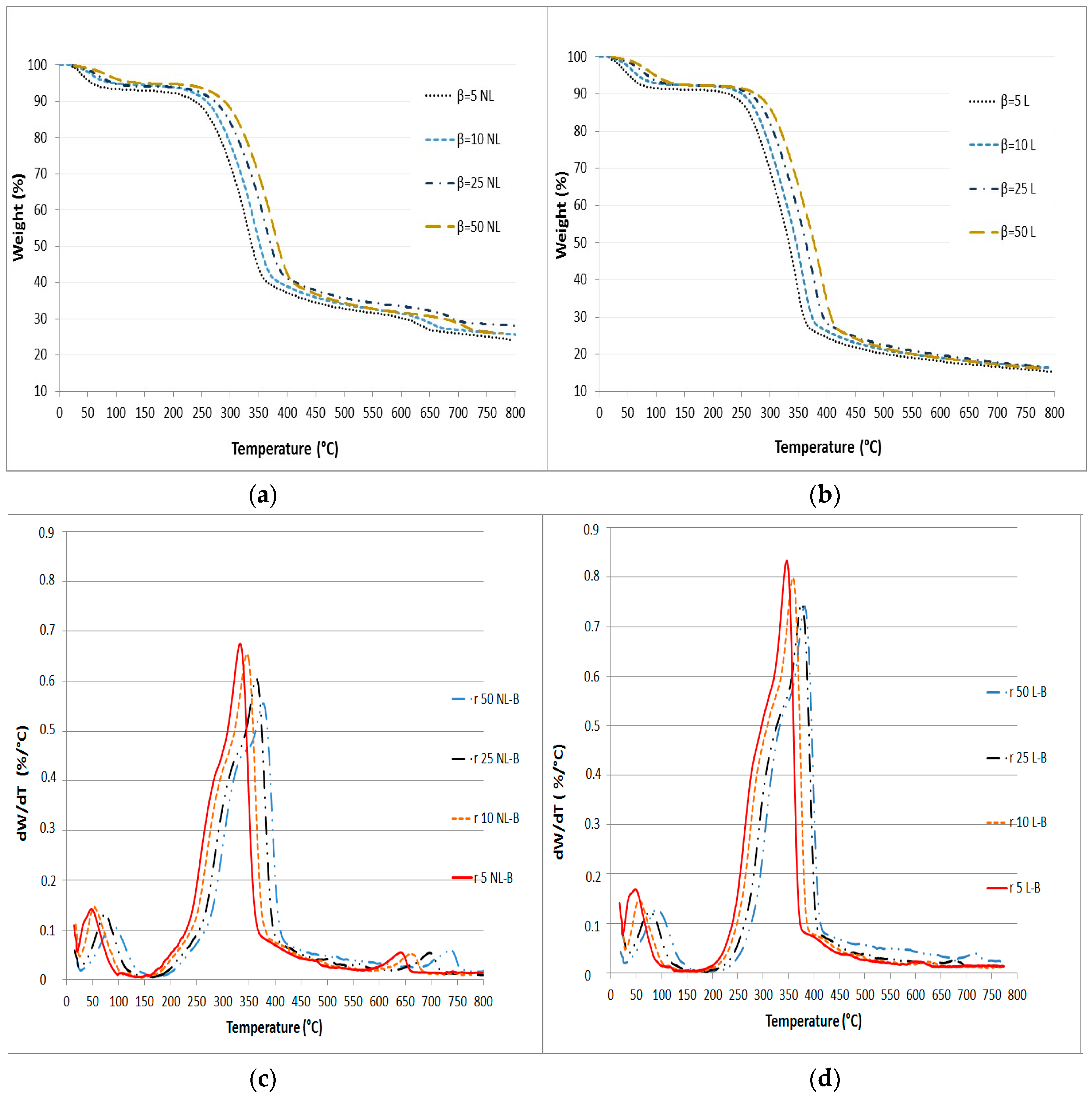
3.1. TG and DTG Analysis

The mass loss (TG) and mass loss rate (DTG) curves for the analyzed biomasses are shown in Figure 1.
The TG curves in Figure 1 enable the comparison of the percentages of unreacted materials and the decomposition profiles for both NL-B and L-B at each heating rate. However, the effect of the heating rate on the mass loss rate of vine wood pyrolysis and the identification of the different components involved in the reaction can be better analyzed by viewing Figure 2.
According to the TGA results, the curves were divided into three zones for NL-B and two main zones for L-B. The first zone extends from room temperature to 150 °C for NL-B, while it extends to 200 °C for L-B. This first zone is related to loss of moisture and the release of some volatile compounds. The second zone is between the end of the first zone and 600 °C. In the DTG curves (Figure 1c,d), this step is characterized by the appearance of a broad peak with one shoulder. The shoulder corresponds to the pyrolysis of cellulose and hemicellulose, while the maximum peak zone is associated with the thermal decomposition of lignin. However, the two steps overlap. At last, the mass loss rate decreases rapidly until reaching 700 °C. Subsequently, the mass loss rate begins to slowly decline, and eventually, its value is close to zero at 800 °C. In the NL-B curve, the last zone corresponds to a further reaction occurring between 600 and 700 °C because of the decomposition of minor components present in the ash; this observation is also reported in the literature [37]. However, this effect is not observed in the L-B curves. This finding may be attributed to the solubility of ash in water during the leaching process. These results are in accordance with those previously reported by Di Blasi in several biomass pyrolysis studies [3]. Finally, the average value of the final residue is about 14% in L-B and 25% in NL-B.
A comparison of the different heating rates in Figure 1 reveals that the maximum value of the mass loss rate is between 330 °C and 400 °C. Meanwhile, both the shoulder and peak are shifted to higher temperatures as the heating rate increases. If both samples are compared, the maximum decomposition ratio is slightly shifted to lower temperatures in NL-biomass. However, this visual effect is attributed to the different percentages of components in the two samples. As a result, although the heating rate affects the peak value and location of the mass loss rate, it has little impact on the tendency of pyrolysis to vary. These results are consistent with those of other studies previously published by Hu, Mishra, and Collard [6,27,33].

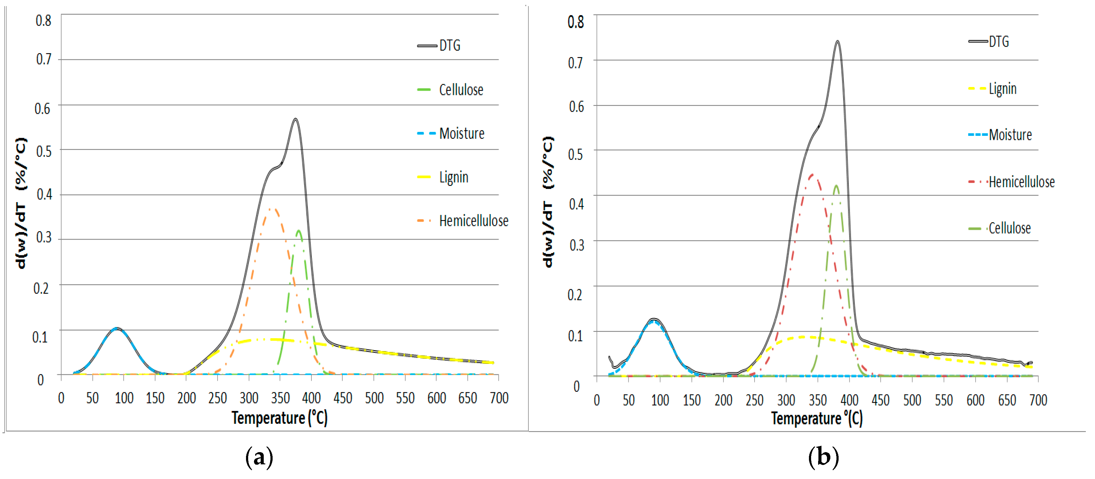
3.2. Figure Deconvolution

In order to better understand and identify the consecutive pyrolysis of the pseudo-components, the DTG figures for both NL-B and L-B were deconvoluted. This transformation was carried out for each heating rate by using Equations (1) and (2). The adjustment parameters were set by using a nonlinear regression model.
The results obtained from DTG deconvolution by applying the Fraser–Suzuki function to the 50 °C/min heating rate are presented in Figure 2. This rate is the only one presented because the other heating rates produce similar results. Therefore, the considered pseudo-components fit the Fraser–Suzuki distribution very well, and this is in accordance with the considerable knowledge of this subject reported in the literature [27,29,31,38,39].
In Figure 2, the individual thermal decomposition of moisture, hemicellulose, cellulose, and lignin is observed in the ranges 25–120, 200–400, 340–400, and 200–600 °C, respectively. Due to its chemical structure, lignin was the most resistant pseudo-component to thermal degradation.
The parameters set by nonlinear regression were adapted to the theoretical relationships obtained in this paper (Equations (4)–(6)), except for the lignin pseudo-component, which can only be correctly adjusted by considering an asymmetric function. These results are consistent with those of other studies and suggest that lignin can be described by more than one function, but only if its overlap generates an asymmetric function. Lastly, the parametrized values of the DTG curves according to the Fraser–Suzuki function are presented in Table 3.
Finally, the relative mass percentages of each pseudo-component were calculated by using the parameters presented in Table 2 and applying Equations (2) and (3). Table 4 provides the results obtained from these calculations. As shown in Table 4, the percentages of cellulose and hemicellulose pseudo-components are higher in L-B than in NL-B. This finding is caused by the reduction in the quantity of some raw material during the leaching process. In addition, the leaching process caused a reduction in the minor components of ash in that sample. Furthermore, a greater reduction in the lignin mass fraction occurred in L-B than in NL-B. This result may be explained by the fact that the finest fraction of material is assumed to be soluble in water.
The weight residuals in Table 4 are related to the amount of biochar obtained after pyrolysis. The differences observed between the values of both weight residuals are related to the lower ash content in the leached biomass.

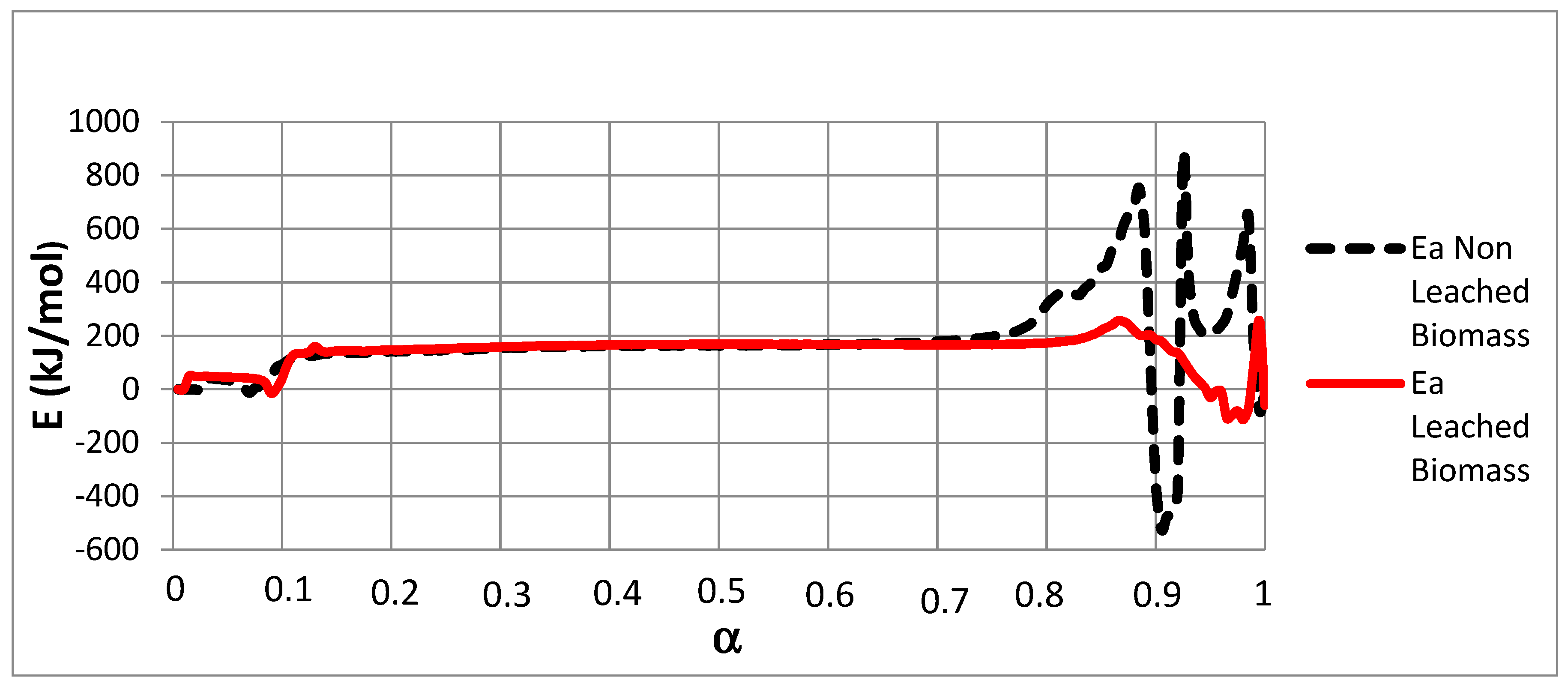
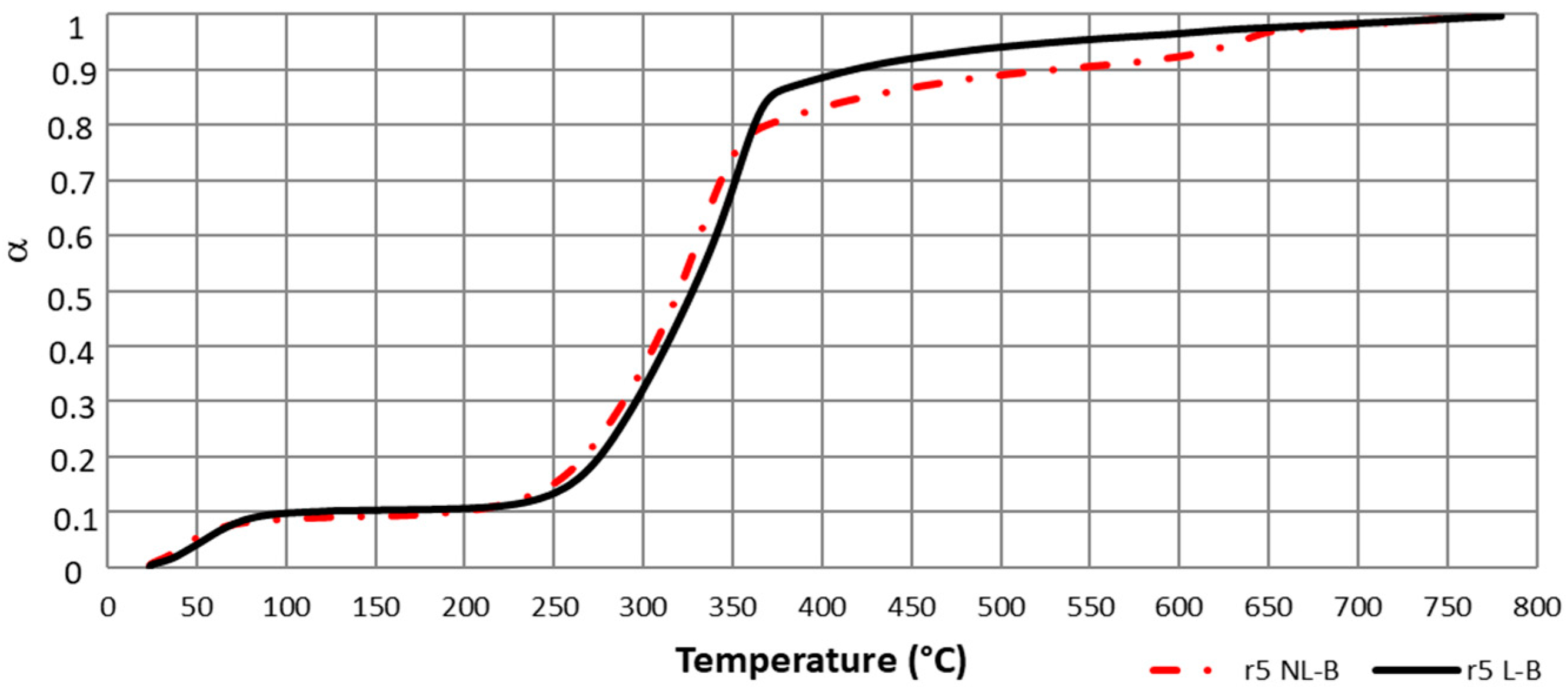
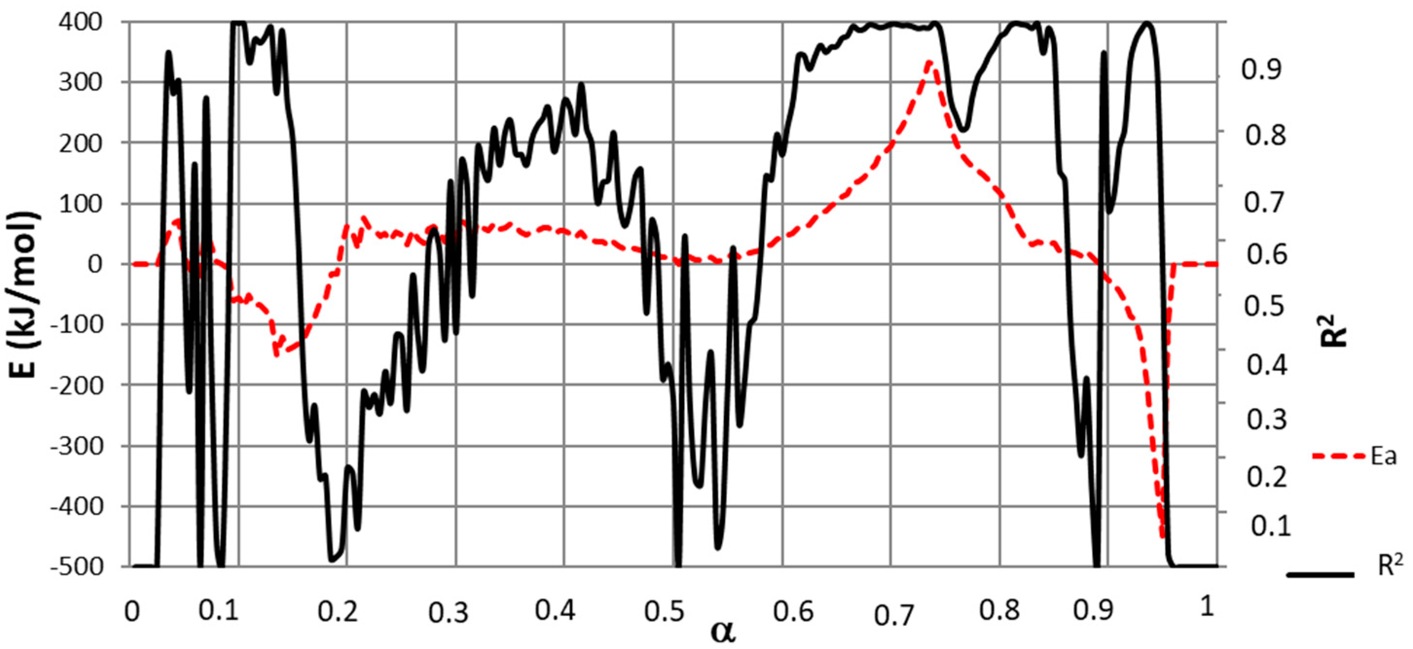
3.3. Isoconversional Method

The activation energy was determined using the Friedman method, which is modeled by Equation (10). The conversion degree values used for calculations ranged between 0.005 and 1. The results obtained by applying the Friedman method are presented in Figure 3 for both NL-B and L-B.
Figure 3 shows that the E values for both samples vary widely within almost the whole range of possible α values. To assess E behavior, the curves were divided into three zones in accordance with increasing α values. The first zone corresponds to the lowest E values (27.7–42.2 kJ/mol). This range is associated with 0 ≤ α ≤ 0.1. The second zone corresponds to intermediate E values (134.9–199.5 kJ/mol) and is associated with 0.1 < α ≤ 0.75. Finally, in both samples, very diverse values are observed from α = 0.75 onward.
This first series of isoconversional data analyses were completed by representing the deconvoluted data by the relationship dα/dt vs. α in order to identify α values for which the reaction could be produced by the thermal pyrolysis of only one pseudo-component. Results are presented in Figure 4 for both NL-B and L-B.
Figure 4 reveals the contribution of different single pseudo-components to dα/dt in the Friedman method. In the range 0 ≤ α < 0.1, the mass reduction is due to only moisture release. This finding agrees with that reported by Font [14], who reported an activation energy below 43.1 kJ/mol for moisture release. In the range 0 ≤ α < 0.8, the main reacting pseudo-component changes for both NL-B and L-B. In this case, pyrolysis of hemicellulose, cellulose, and lignin occurs simultaneously. These results were also observed in a 2016 study by Hu et al. [27], who reported activation energy values between 152.43 and 210.39 kJ/mol for pine wood, rice husk, and bamboo. In addition, Mishra and Mohanty published several activation energy values in a review of 16 different biomasses [33]. In their work, the values reported were between 106.5 and 184.61 kJ/mol by applying the same Friedman method.
At α ≅ 0.8, hemicellulose, cellulose, and lignin contribute to the total decomposition in both samples, with no single component having a clear predominant role. In addition, the decomposition of cellulose and hemicellulose is always accompanied by other reactions. However, in the last reaction step, the contribution to dα/dt in the Friedman method clearly corresponds to the pyrolysis of a single pseudo-component: lignin. This finding is observed in the range 0.84 ≤ α ≤ 0.9 for NL-B and α > 0.9 for L-B.
The variation in the ranges of α value in which each pseudo-component is the main reacting component in the pyrolysis can be explained by the differences in unreacted material between the two biomasses. This causes a delay in conversion degree when comparing NL-B and L-B. Further analysis of this item is seen in Figure 5; because of the similarities for all heating ramps, only 5 °C/min is presented.
Therefore, because α values were found to be dependent on the unreacted material, it can be concluded that the selected α range values applied to the isoconversional methods strongly depend on the sample, even for similar biomasses. As a consequence, E values were obtained by applying the Friedman method not only to deconvoluted data but also to Equation (13) by using the previously identified delay in conversion degree shown in Figure 5.
To implement calculations and as a result of the observed lag in the decomposition of cellulose and lignin, Equations (12) and (13) were used with different α values for both NL-B and L-B samples for zones in which a single pseudo-component was decomposing. The resulting activation energy values are presented in Figure 6, which shows a lag in the conversion degree of 0.05 in L-B with respect to NL-B.
The correlation coefficient (R2) from fitting Equation (12) (and, consequently, Equation (13)) is also presented in Figure 6. This parameter shows the goodness of the fit. It can be concluded from Figure 6 that high R2 values are obtained in zones in which a single pseudo-component was decomposing. In addition, the range of α values in which a high R2 coefficient is obtained coincides with those determined in Figure 4.
If E values are associated with α ranges, the following results apply: moisture release at 0.03 ≤ α ≤ 0.08 (NL-B) and (0.03 + ∆α) ≤ α ≤ (0.08 + ∆α) (L-B); cellulose pyrolysis at 0.73 ≤ α ≤ 0.8 (NL-B) and (0.73 + ∆α) ≤ α ≤ (0.8 + ∆α) (L-B); and lignin decomposition at 0.82 ≤ α ≤ 0.89 (NL-B) and (0.82 + ∆α) ≤ α ≤ (0.89 + ∆α) (L-B). For zones that are not included in the previous list of ranges, the degradation of a single-pseudo-component was not observed. As a consequence, these zones do not allow for the identification of any common E values for either NL-B or L-B samples. It seems somewhat surprising that no E values were found in these conditions because Figure 3 presents stable values with a good mathematic correlation in those zones. However, a straight line from Equation (11) cannot be constructed when several components react simultaneously. Hence, E values diverge, and low R2 coefficients are obtained.
Contrary to initial expectations, Figure 6 reports some negative E values. Although unexpected, this finding was also reported by Yeo et al. [12], and it is attributed to complex reversible reactions or dominant diffusion processes.
Finally, in order to compare the applied methods, the ranges of E and α values for each pseudo-component are presented in Table 5.
The findings shown in Table 5 are consistent with those of Font and Garrido [14], Yeo et al. [12], Mamleev et al. [40], Hu et al. [27], Mishra and Mohanty [33], and Fiori et al. [41], who found similar E values to those reported herein for each pseudo-component or for the conversion degree in biomass pyrolysis. However, there are some differences between the results reported here and those reported by Osman et al. [19], who obtained E ranging from 40 to 165 kJ/mol for miscanthus pyrolysis. As a result, the procedure followed in this paper was shown to be valid for studying pyrolysis biomass kinetics.

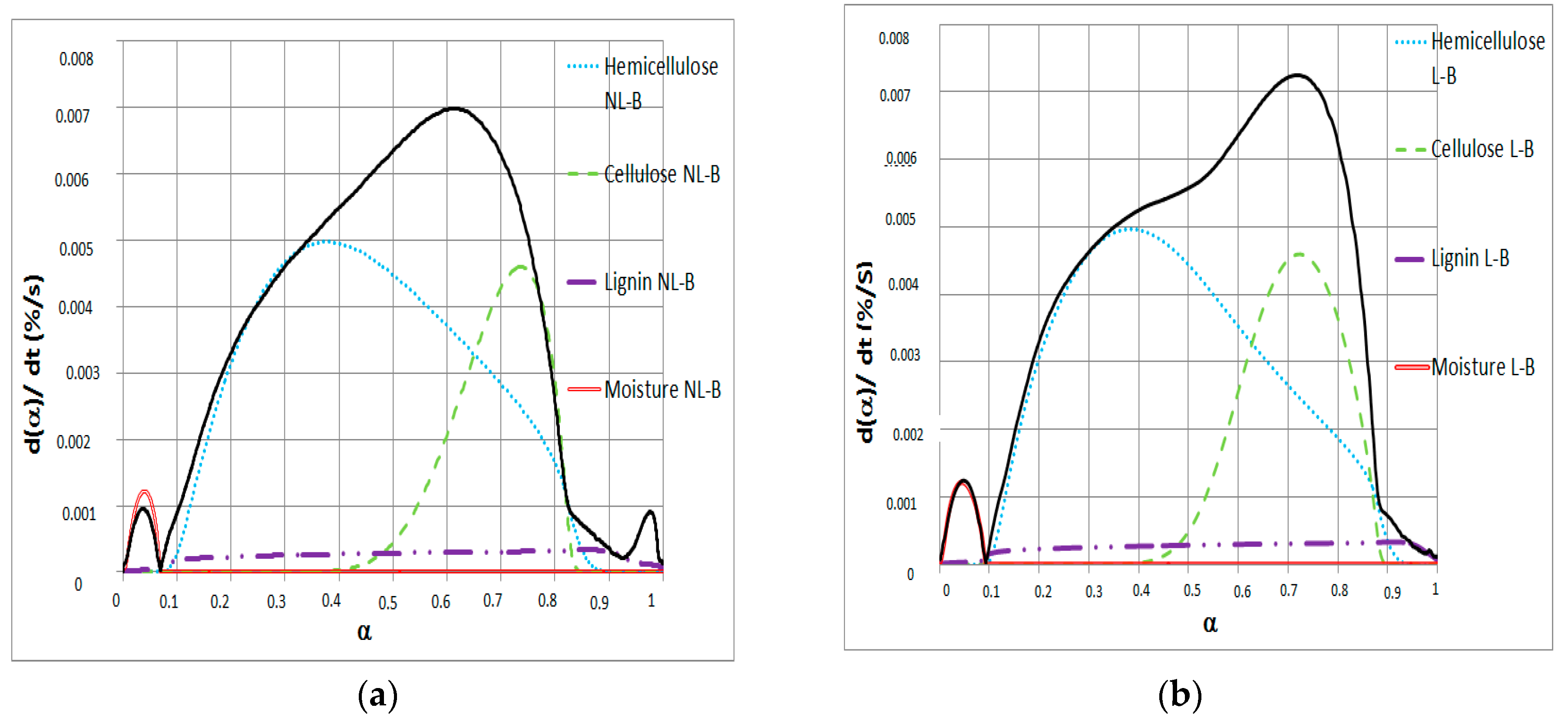
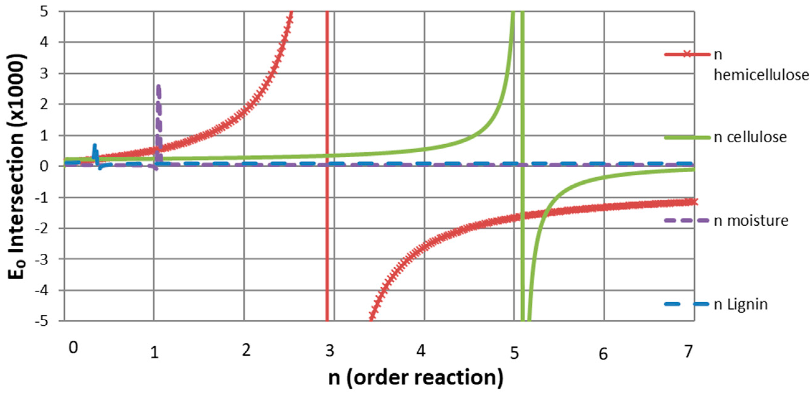
3.4. Reaction Model Determination

The results of applying the Avrami Erofeev model are presented in Figure 7. A wide range of n α values, from 0.025 to 7, were computed, and E0 values obtained by the intersection of the CE lines of both samples were plotted for each n value. Some discontinuities are observed in Figure 7, and they indicate the n values at which both CE lines are parallel. Hence, the n values at these points represent the reaction order of each pseudo-component’s pyrolysis.
As a result, common first-, third-, and fifth-order reactions were approximated for moisture, hemicellulose, and cellulose, while an n non-integer common order reaction of 0.35 was obtained for lignin. Although these results differ from some published reaction orders for cellulose [12,27], they are consistent with those of hemicellulose and lignin. As the two cited works disagree on cellulose’s reaction order, and since the present work shows a good fit and simulation of the TG curves, the cellulose kinetic parameters are accepted.

4. Conclusions

Common kinetic parameters were calculated by using the classic Friedman method and the Fraser–Suzuki deconvolution technique for both non-leached and leached biomasses. Hemicellulose and cellulose were satisfactorily adjusted by a symmetric function, whereas lignin was fit by an asymmetric function. Although it was possible to obtain the activation energy values by applying the classic Friedman method, the individual Friedman method based on deconvolution data showed that it was not possible to directly apply Friedman relationships to all pseudo-components, indicating that more pseudo-components during the deconvolution or other adjustment models must be used in the process. As a consequence, the first important finding of this study is that the classic Friedman method does not seem to be a good technique to study how heterogeneous biomass pyrolysis occurs. As a result, the classic Friedman isoconversional method was found to be strongly dependent on the sample, even for similar biomasses; thus, this technique is not powerful enough to study heterogeneous material pyrolysis.
However, a Friedman isoconversional method that was modified by applying the delay in conversion degree was studied, and the application of other isoconversional methods based on nonlinear fittings allowed for the determination of kinetic parameters that are not dependent on each pseudo-component’s percentage of the biomass. Hence, the most obvious finding to emerge from this study is that the deconvolution technique coupled to the delay in conversion degree improves the ability to compare the pyrolysis degradation of two heterogeneous biomasses.

Author Contributions

All authors made substantial contributions to the conception or design of this work and took part in data acquisition, analysis, and its interpretation. All of them drafted the work and substantively revised it. All authors approve of the submitted version (and the version substantially edited by journal staff that involves the author’s contribution to the study) and agree to be personally accountable for their own contributions and for ensuring that questions related to the accuracy or integrity of any part of the work are appropriately investigated, resolved, and documented in the literature.

Funding

This research received no external funding.

Acknowledgments

This research was supported by the Natural Resources Institute of Universidad de León, which provided human and material assistance.

Conflicts of Interest

The authors declare no conflict of interest.

References

  1. UNFCCC, Global Warming of 1.5 °C Special Report. 2018. Available online: https://www.ipcc.ch/sr15/ (accessed on 29 December 2018).
  2. UNFCCC, 2016 Earth Information Day. 2016. Available online: http://unfccc.int/science/workstreams/items/9949.php (accessed on 29 December 2018).
  3. Diblasi, C. Modeling chemical and physical processes of wood and biomass pyrolysis. Prog. Energy Combust. Sci. 2008, 34, 47–90. [Google Scholar] [CrossRef]
  4. Rentizelas, A.A.; Li, J. Techno-economic and carbon emissions analysis of biomass torrefaction downstream in international bioenergy supply chains for co-firing. Energy 2016, 114, 129–142. [Google Scholar] [CrossRef] [Green Version]
  5. Leng, L.; Huang, H. An overview of the effect of pyrolysis process parameters on biochar stability. Bioresour. Technol. 2018, 270, 627–642. [Google Scholar] [CrossRef] [PubMed]
  6. Collard, F.-X.; Blin, J. A review on pyrolysis of biomass constituents: Mechanisms and composition of the products obtained from the conversion of cellulose, hemicelluloses and lignin. Renew. Sustain. Energy Rev. 2014, 38, 594–608. [Google Scholar] [CrossRef]
  7. Chen, Z.; Wang, M.; Jiang, E.; Wang, D.; Zhang, K.; Ren, Y.; Jiang, Y. Pyrolysis of Torrefied Biomass. Trends Biotechnol. 2018, 36, 1287–1298. [Google Scholar] [CrossRef] [PubMed] [Green Version]
  8. Wei, S.; Zhu, M.; Fan, X.; Song, J.; Peng, P.; Li, K.; Jia, W.; Song, H. Influence of pyrolysis temperature and feedstock on carbon fractions of biochar produced from pyrolysis of rice straw, pine wood, pig manure and sewage sludge. Chemosphere 2019, 218, 624–631. [Google Scholar] [CrossRef] [PubMed]
  9. López, R.; Fernández, C.; Gómez, X.; Martínez, O.; Sánchez, M.E. Thermogravimetric analysis of lignocellulosic and microalgae biomasses and their blends during combustion. J. Therm. Anal. Calorim. 2013, 114, 295–305. [Google Scholar] [CrossRef]
  10. Criado, J.M.; Sánchez-Jiménez, P.E.; Perez-Maqueda, L.A. Critical study of the isoconversional methods of kinetic analysis. J. Therm. Anal. Calorim. 2008, 92, 199–203. [Google Scholar] [CrossRef] [Green Version]
  11. Kalogiannis, K.G.; Matsakas, L.; Lappas, A.A.; Rova, U.; Christakopoulos, P. Aromatics from Beechwood Organosolv Lignin through Thermal and Catalytic Pyrolysis. Energies 2019, 12, 1606. [Google Scholar] [CrossRef]
  12. Yeo, J.Y.; Chin, B.L.F.; Tan, J.K.; Loh, Y.S. Comparative studies on the pyrolysis of cellulose, hemicellulose, and lignin based on combined kinetics. J. Energy Inst. 2017. [Google Scholar] [CrossRef]
  13. Song, E.; Kim, D.; Jeong, C.-J.; Kim, D.-Y. A Kinetic Study on Combustible Coastal Debris Pyrolysis via Thermogravimetric Analysis. Energies 2019, 12, 836. [Google Scholar] [CrossRef]
  14. Font, R.; Garrido, M. Friedman and n-reaction order methods applied to pine needles and polyurethane thermal decompositions. Thermochim. Acta 2018, 660, 124–133. [Google Scholar] [CrossRef] [Green Version]
  15. Braga, R.M.; Melo, D.M.A.; Aquino, F.M.; Freitas, J.C.O.; Melo, M.A.F.; Barros, J.M.F.; Fontes, B.M.S. Characterization and comparative study of pyrolysis kinetics of the rice husk and the elephant grass. J. Therm. Anal. Calorim. 2014, 115, 1915–1920. [Google Scholar] [CrossRef]
  16. Sanchez, M.; Otero, M.; Gómez, X.; Moran, A. Thermogravimetric kinetic analysis of the combustion of biowastes. Renew. Energy 2009, 34, 1622–1627. [Google Scholar] [CrossRef]
  17. White, J.E.; Catallo, W.J.; Legendre, B.L. Biomass pyrolysis kinetics: A comparative critical review with relevant agricultural residue case studies. J. Anal. Appl. Pyrolysis 2011, 91, 1–33. [Google Scholar] [CrossRef]
  18. Jiang, G.; Nowakowski, D.J.; Bridgwater, A.V. A systematic study of the kinetics of lignin pyrolysis. Thermochim. Acta 2010, 498, 61–66. [Google Scholar] [CrossRef]
  19. Osman, A.I.; Abdelkader, A.; Johnston, C.R.; Morgan, K.; Rooney, D.W. Thermal Investigation and Kinetic Modeling of Lignocellulosic Biomass Combustion for Energy Production and Other Applications. Ind. Eng. Chem. Res. 2017, 56, 12119–12130. [Google Scholar] [CrossRef] [Green Version]
  20. Várhegyi, G.; Antal, M.J.; Jakab, E.; Szabó, P. Kinetic modeling of biomass pyrolysis. 10 years of a US-Hungarian cooperation. J. Anal. Appl. Pyrolysis 1997, 42, 73–87. [Google Scholar] [CrossRef]
  21. Szabó, P.; Várhegyi, G.; Till, F.; Faix, O. Thermogravimetric/mass spectrometric characterization of two energy crops, Arundo donax and Miscanthus sinensis. J. Anal. Appl. Pyrolysis 1996, 36, 179–190. [Google Scholar] [CrossRef]
  22. Liu, H.; Zhang, L.; Han, Z.; Xie, B.; Wu, S. The effects of leaching methods on the combustion characteristics of rice straw. Biomass-Bioenergy 2013, 49, 22–27. [Google Scholar] [CrossRef]
  23. Kong, Z.; Liaw, S.B.; Gao, X.; Yu, Y.; Wu, H. Leaching characteristics of inherent inorganic nutrients in biochars from the slow and fast pyrolysis of mallee biomass. Fuel 2014, 128, 433–441. [Google Scholar] [CrossRef]
  24. Haykiri-Acma, H. The role of particle size in the non-isothermal pyrolysis of hazelnut shell. J. Anal. Appl. Pyrolysis 2006, 75, 211–216. [Google Scholar] [CrossRef]
  25. Cai, J.; Wu, W.; Liu, R. An overview of distributed activation energy model and its application in the pyrolysis of lignocellulosic biomass. Renew. Sustain. Energy Rev. 2014, 36, 236–246. [Google Scholar] [CrossRef]
  26. Liu, S.; Yu, J.; Bikane, K.; Chen, T.; Ma, C.; Wang, B.; Sun, L. Rubber pyrolysis: Kinetic modeling and vulcanization effects. Energy 2018, 155, 215–225. [Google Scholar] [CrossRef]
  27. Hu, M.; Chen, Z.; Wang, S.; Guo, D.; Ma, C.; Zhou, Y.; Chen, J.; Laghari, M.; Fazal, S.; Xiao, B.; et al. Thermogravimetric kinetics of lignocellulosic biomass slow pyrolysis using distributed activation energy model, Fraser–Suzuki deconvolution, and iso-conversional method. Energy Convers. Manag. 2016, 118, 1–11. [Google Scholar] [CrossRef]
  28. Díaz, I.; Rodríguez, M.; Arnaiz, C.; Miguel, G.S.; Domínguez, M. Biomass pyrolysis kinetics through thermogravimetric analysis. Comput. Aided Chem. Eng. 2013, 32, 1–6. [Google Scholar] [CrossRef]
  29. Perejón, A.; Sánchez-Jiménez, P.E.; Criado, J.M.; Pérez-Maqueda, L.A. Kinetic analysis of complex solid-state reactions. A new deconvolution procedure. J. Phys. Chem. B 2011, 115, 1780–1791. [Google Scholar] [CrossRef] [PubMed]
  30. Moine, E.C.; Groune, K.; El Hamidi, A.; Khachani, M.; Halim, M.; Arsalane, S. Multistep process kinetics of the non-isothermal pyrolysis of Moroccan Rif oil shale. Energy 2016, 115, 931–941. [Google Scholar] [CrossRef]
  31. Cheng, Z.; Wu, W.; Ji, P.; Zhou, X.; Liu, R.; Cai, J. Applicability of Fraser-Suzuki function in kinetic analysis of DAEM processes and lignocellulosic biomass pyrolysis processes. J. Therm. Anal. Calorim. 2015, 119, 1429–1438. [Google Scholar] [CrossRef]
  32. Svoboda, R.; Málek, J. Applicability of Fraser–Suzuki function in kinetic analysis of complex crystallization processes. J. Therm. Anal. Calorim. 2013, 111, 1045–1056. [Google Scholar] [CrossRef]
  33. Mishra, R.K.; Mohanty, K. Pyrolysis kinetics and thermal behavior of waste sawdust biomass using thermogravimetric analysis. Bioresour. Technol. 2018, 251, 63–74. [Google Scholar] [CrossRef]
  34. Qiao, Y.; Zhang, L.; Binner, E.; Xu, M.; Li, C.-Z. An investigation of the causes of the difference in coal particle ignition temperature between combustion in air and in O2/CO2. Fuel 2010, 89, 3381–3387. [Google Scholar] [CrossRef]
  35. Tian, L.; Shen, B.; Xu, H.; Li, F.; Wang, Y.; Singh, S. Thermal behavior of waste tea pyrolysis by TG-FTIR analysis. Energy 2016, 103, 533–542. [Google Scholar] [CrossRef]
  36. Vyazovkin, S.; Burnham, A.K.; Criado, J.M.; Pérez-Maqueda, L.A.; Popescu, C.; Sbirrazzuoli, N. ICTAC Kinetics Committee recommendations for performing kinetic computations on thermal analysis data. Thermochim. Acta 2011, 520, 1–19. [Google Scholar] [CrossRef]
  37. Vargas-Moreno, J.; Callejon-Ferre, A.J.; Pérez-Alonso, J.; Marti, B.V. A review of the mathematical models for predicting the heating value of biomass materials. Renew. Sustain. Energy Rev. 2012, 16, 3065–3083. [Google Scholar] [CrossRef]
  38. Stefanidis, S.D.; Kalogiannis, K.G.; Iliopoulou, E.F.; Michailof, C.M.; Pilavachi, P.A.; Lappas, A.A. A study of lignocellulosic biomass pyrolysis via the pyrolysis of cellulose, hemicellulose and lignin. J. Anal. Appl. Pyrolysis 2014, 105, 143–150. [Google Scholar] [CrossRef]
  39. Chen, C.; Miao, W.; Zhou, C.; Wu, H. Thermogravimetric pyrolysis kinetics of bamboo waste via Asymmetric Double Sigmoidal (Asym2sig) function deconvolution. Bioresour. Technol. 2017, 225, 48–57. [Google Scholar] [CrossRef]
  40. Mamleev, V.; Bourbigot, S.; Yvon, J. Kinetic analysis of the thermal decomposition of cellulose: The main step of mass loss. J. Anal. Appl. Pyrolysis 2007, 80, 151–165. [Google Scholar] [CrossRef]
  41. Fiori, L.; Valbusa, M.; Lorenzi, D.; Fambri, L. Modeling of the devolatilization kinetics during pyrolysis of grape residues. Bioresour. Technol. 2012, 103, 389–397. [Google Scholar] [CrossRef]
Figure 1. TG curves for (a) NL-B and (b) L-B samples and derivative TG (DTG) curves for (c) NL-B and (d) L-B at different heating rates.
Energies 12 02599 g001
Figure 2. Deconvolution for (a) NL-B and (b) L-B at a 50 °C/min heating ramp.
Energies 12 02599 g002
Figure 3. E versus α using the Friedman method for NL-B and L-B samples.
Energies 12 02599 g003
Figure 4. dα/dt versus α for (a) NL-B and (b) L-B samples at 50 °C/min heating ramp.
Energies 12 02599 g004
Figure 5. Delay in α (T) for NL-B and L-B samples for a 5 °C/min heating ramp.
Energies 12 02599 g005
Figure 6. Common E with the Friedman method with a delay of α = 0.05 in both samples by using Equation (13).
Energies 12 02599 g006
Figure 7. Common n-order reaction for each pseudo-component.
Energies 12 02599 g007
Table 1. Particle size distribution of non-leached biomass (NL-B) and leached biomass (L-B) samples.
Particle Size (mm)X < 11 < X < 22 < X < 44 < X < 88 < X < 10X > 10
NL-B13.4%7.4%10.8%19.7%13.5%35.2%
L-B0%8.6%12.4%22.7%15.6%40.7%
Table 2. Proximate analysis of leached and non-leached biomass samples.
Parameter (%)MoistureVolatile *Ash *Fixed Carbon **HHV (MJ/kg)
NL-B9.0070.8013.5515.6516.51
L-B3.4782.771.4715.7618.87
* Dry basis. ** Calculated by difference.
Table 3. Deconvolution parameters of each pseudo-component for both samples.
Parameter50 °C/min25 °C/min10 °C/min5 °C/min
L-BNL-BL-BNL-BL-BNL-BL-BNL-B
Moistureh0.1110.1030.1160.1180.1170.1130.1610.144
s0.0010.0010.0010.0010.0010.0010.0010.001
p89.31589.31574.96974.96948.11348.11340.05040.050
w62.81562.91162.00062.00062.89862.89862.81562.815
Hemicelluloseh0.4860.3800.4590.3510.4620.3830.4500.383
s0.0000.0000.0000.0000.0000.0000.0000.000
p342.318337.844326.503326.184313.099313.099307.318307.318
w75.25175.18175.71175.49675.11175.09175.25175.091
Celluloseh0.4910.3200.4910.4050.4950.3900.4910.390
s0.0000.0000.0000.0000.0000.0000.0000.000
p383.249379.693375.693372.208355.125355.125343.249343.249
w34.39934.60434.58435.55834.51034.57334.39934.573
Ligninh0.0670.0790.0670.0790.0720.0820.0670.082
s1.0001.0001.0001.0001.0001.0001.0001.000
p329.587329.587295.000295.000264.204264.204260.000260.000
w265.835293.415212.920243.415164.061210.767180.835210.767
Table 4. Relative percentages of each pseudo-component for both samples.
(%)Leached BiomassNon-Leached Biomass
Moisture7.87 ± 0.577.60 ± 0.44
Cellulose14.01 ± 1.0911.18 ± 1.72
Hemicellulose36.43 ± 0.5530.41 ± 0.39
Lignin20.14 ± 3.0323.24 ± 1.78
Minor components of Ash0.62 ± 1.001.92 ± 0.47
Total Reaction79.07 ± 6.2474.36 ± 4.80
Weight Residual20.93 ± 6.2425.64 ± 4.80
Table 5. Ranges of α and E values obtained for each pseudo-component.
Classic Friedman MethodFriedman Method to Deconvoluted DataDelay Friedman Method with α = 0.05
Pseudo-componentE (kJ/mol)Range of α selectedE (kJ/mol)E (kJ/mol)Range of α selected (L-B)
Moisture36.1–49.70.025–0.06546.8–51.949.2–57.70.035–0.065
Hemicellulose125.4–146.50.123–0.240182.8–223.6(−55.1) to (−67.6)0.123–0.240
Cellulose168.3–212.10.670–0.770187.4–231.2338.0–356.40.735–0.795
Ligninunstable0.850–0.91071.7–85.433.3–48.30.860–0.890

