Influence of Inclined Magnetic Field on Carreau Nanoliquid Thin Film Flow and Heat Transfer with Graphene Nanoparticles

 ,
,  ,
,  , , ,
, , ,
Abstract
:1. Introduction
2. Materials and Method
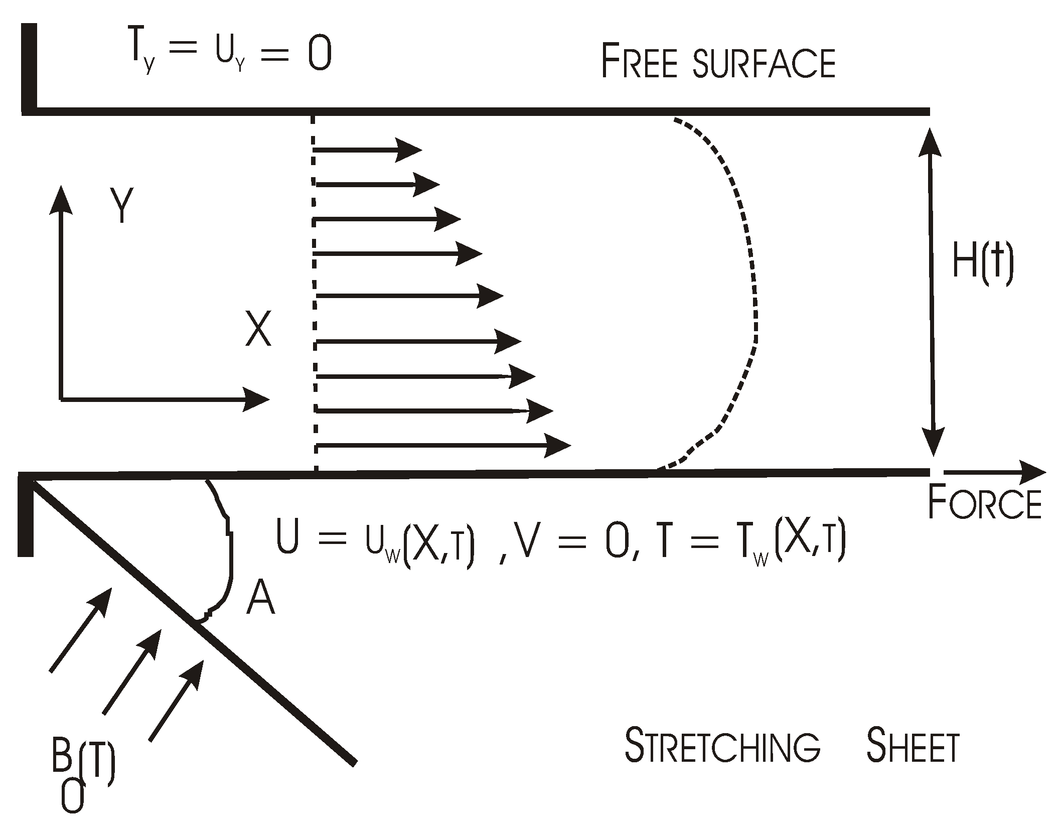
Problem Formulation
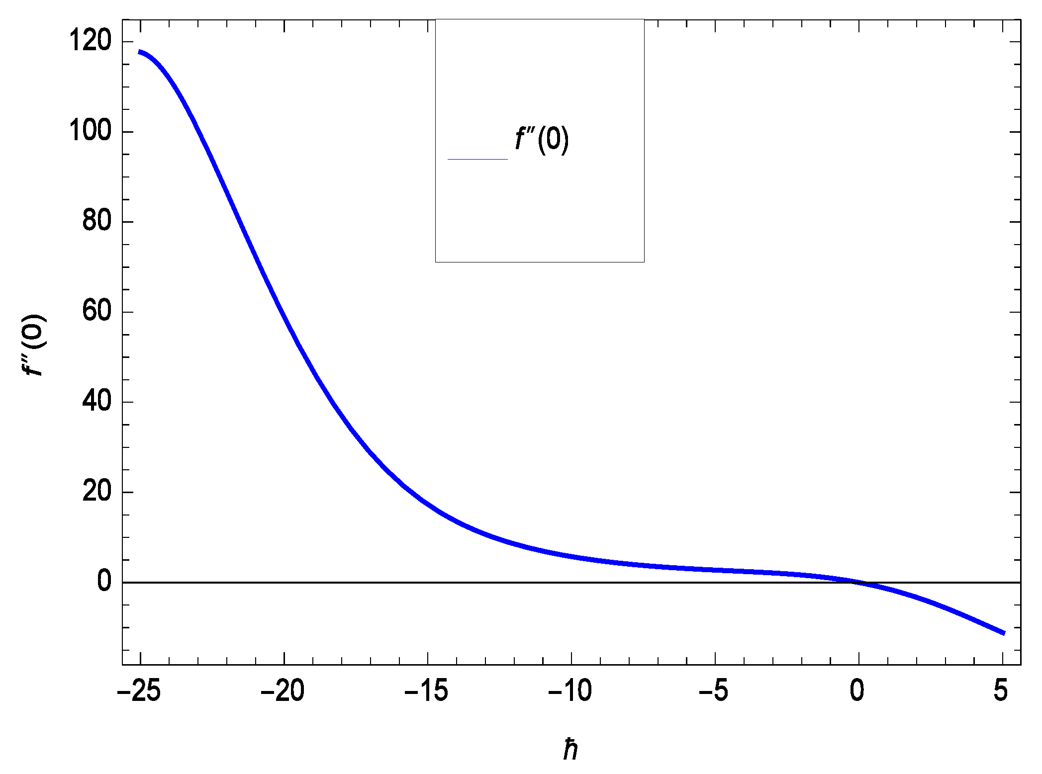
3. Computation of the Transformed Equations Via HAM
3.1. Zeroth-Order Deformation Problems
3.2. mth-Order Deformation Problems
4. Results and Discussion
5. Discussion
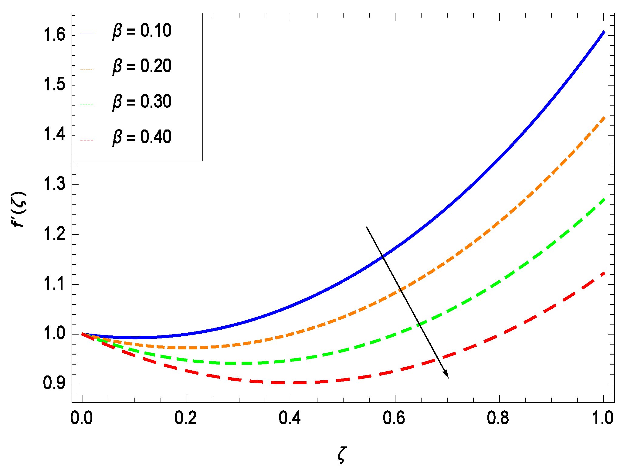
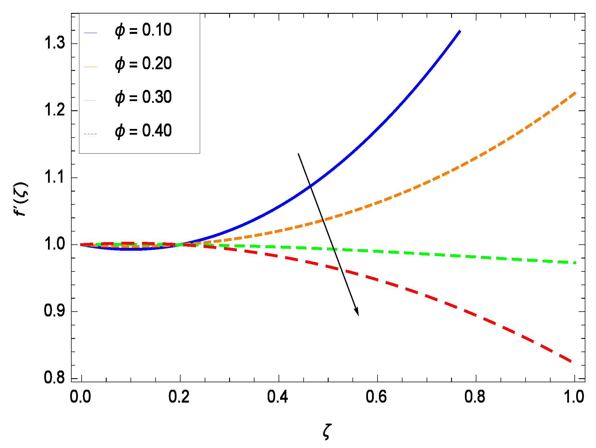
5.1. Velocity Profile
5.2. Temperature Profile
5.3. Comparison of the Present Work
6. Conclusions
- (1)
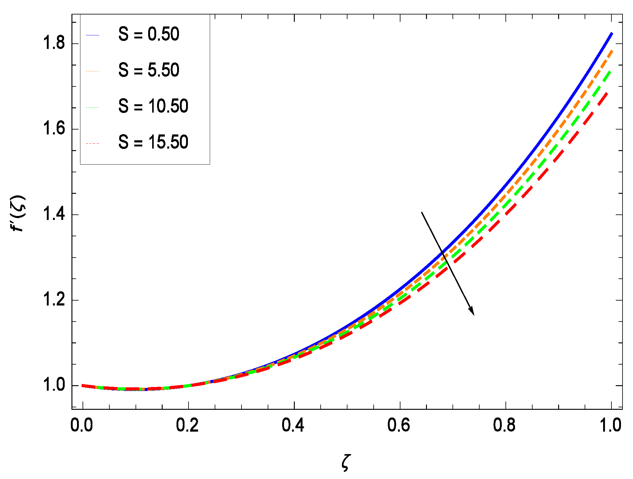
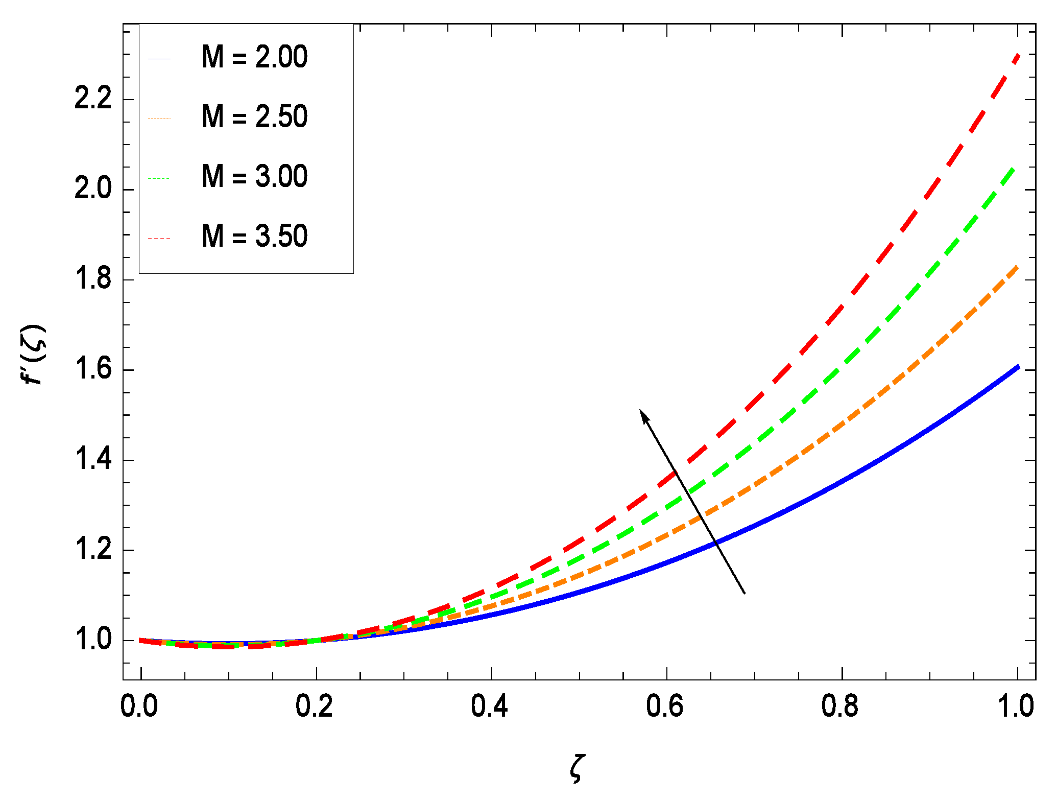
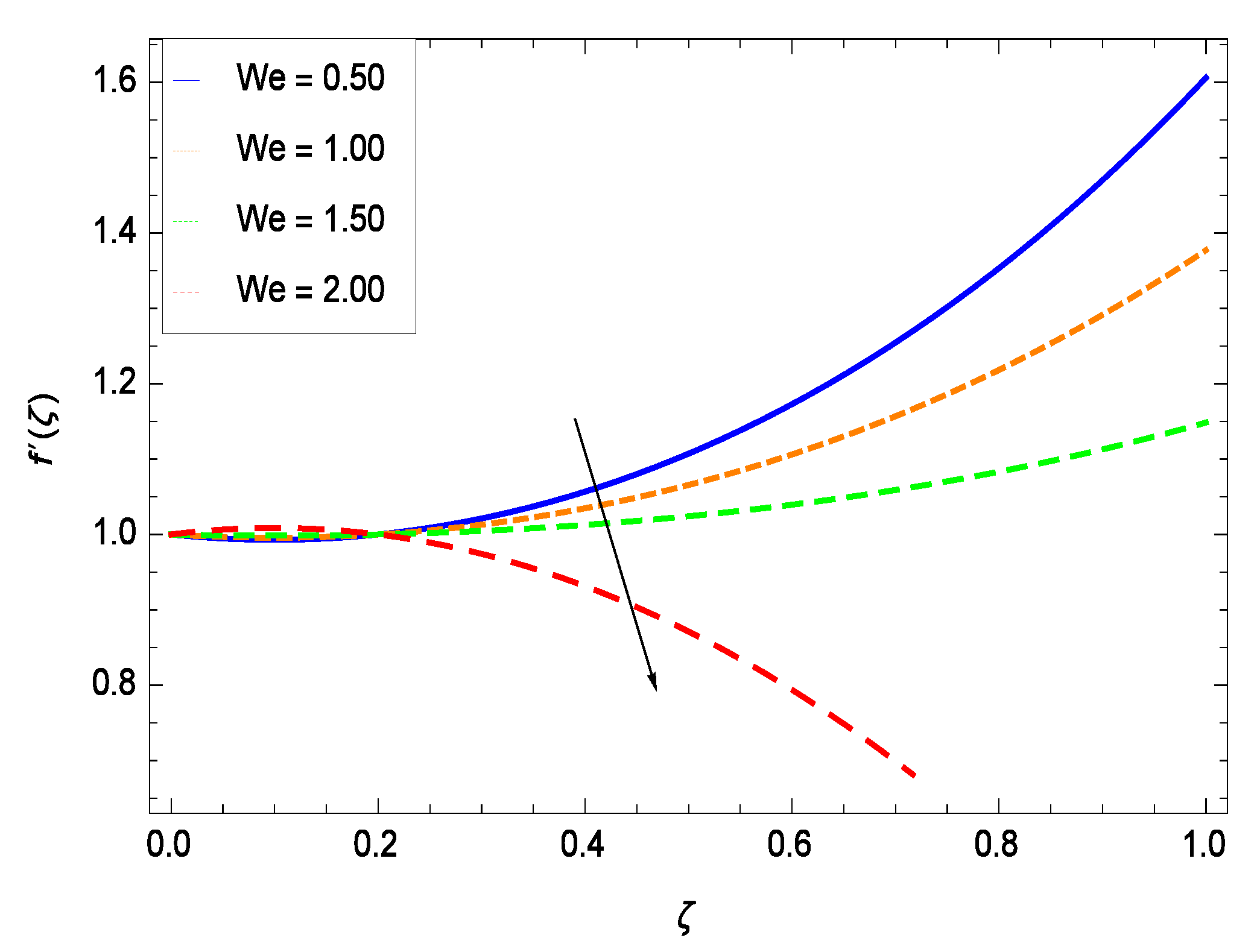
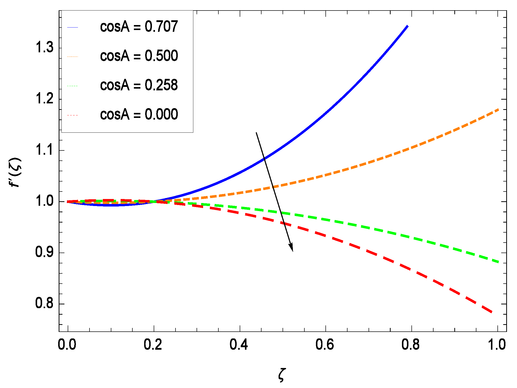
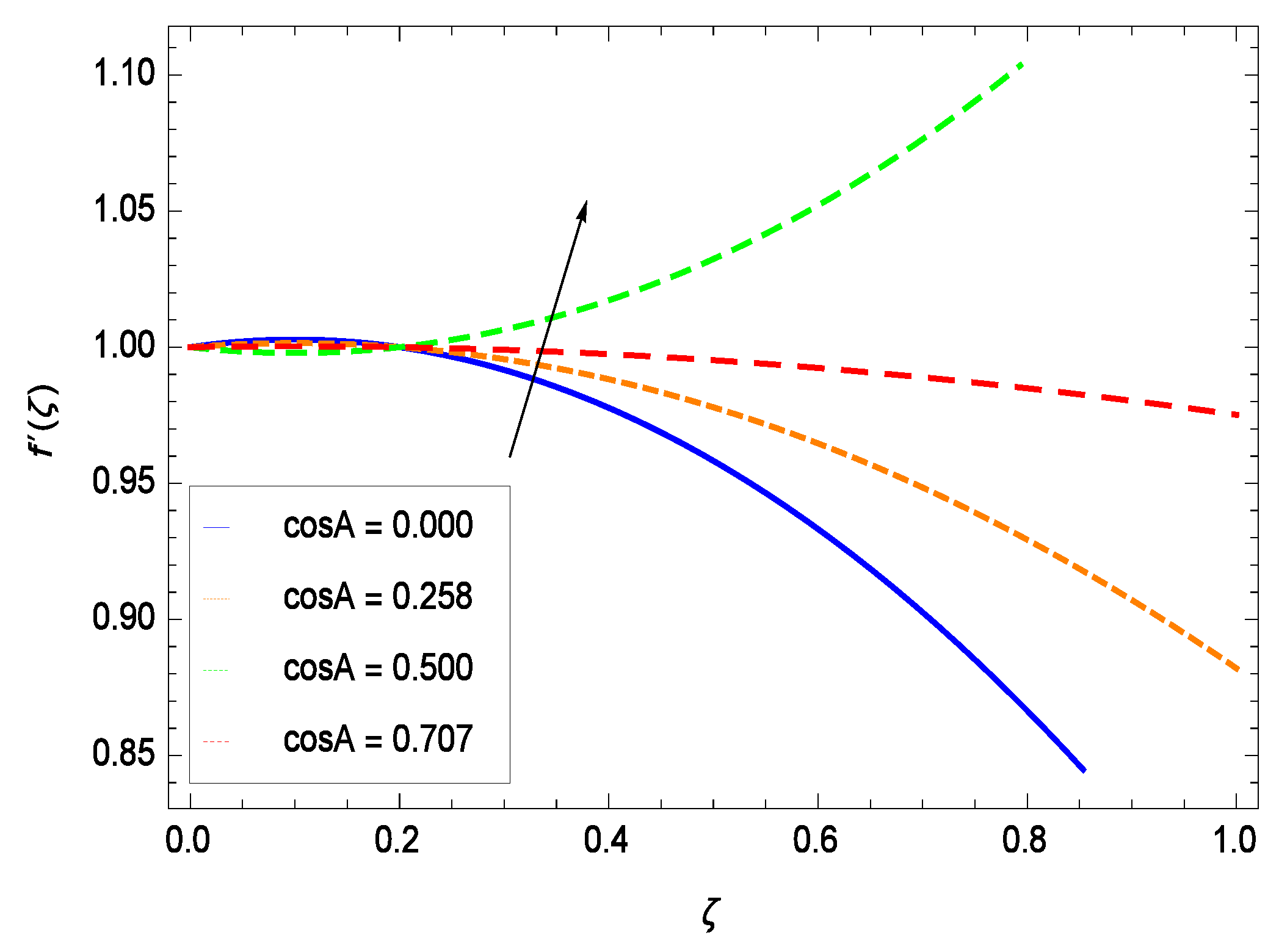
- The velocity f’() decreases with , , S, n, We, and increasing A, and increases with M and reducing A.
- (2)
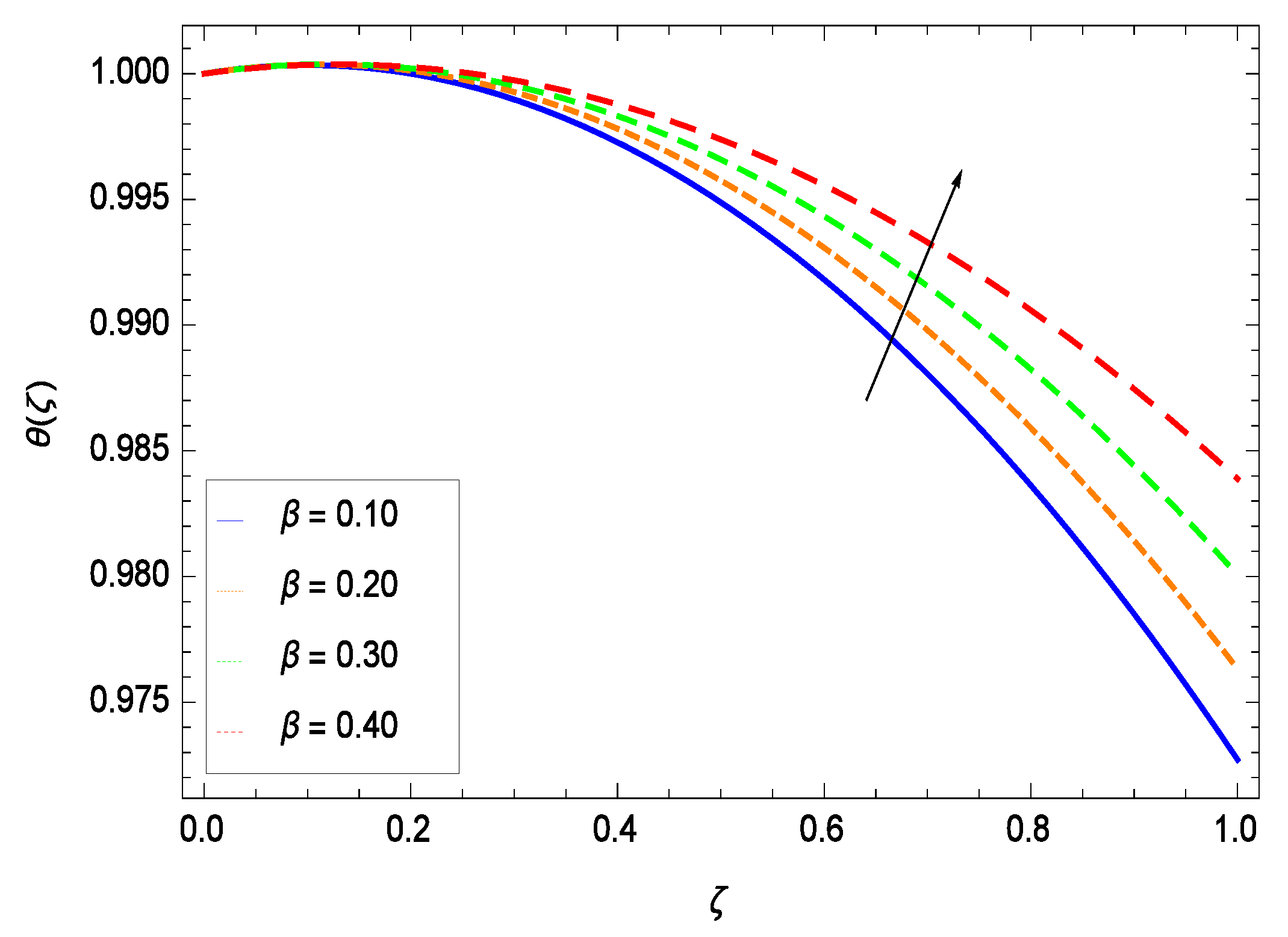
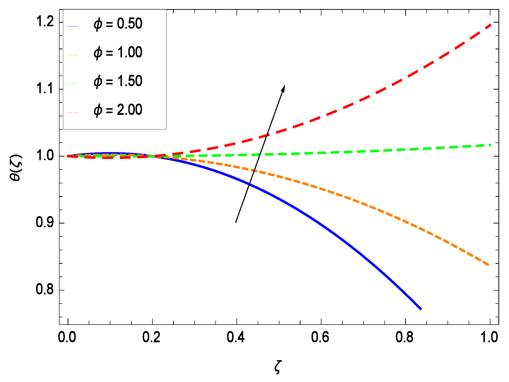
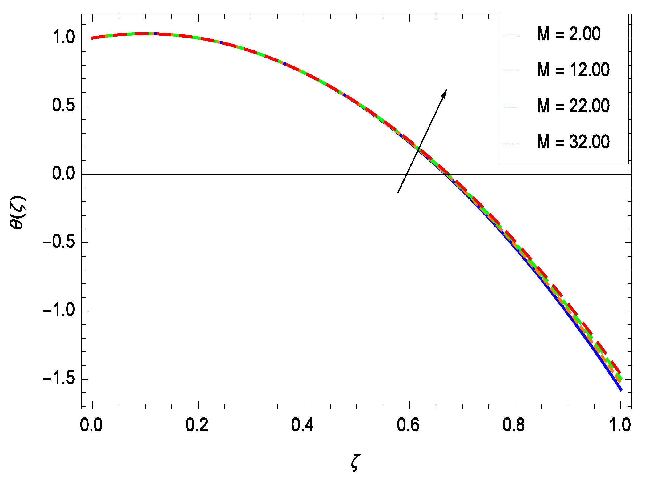
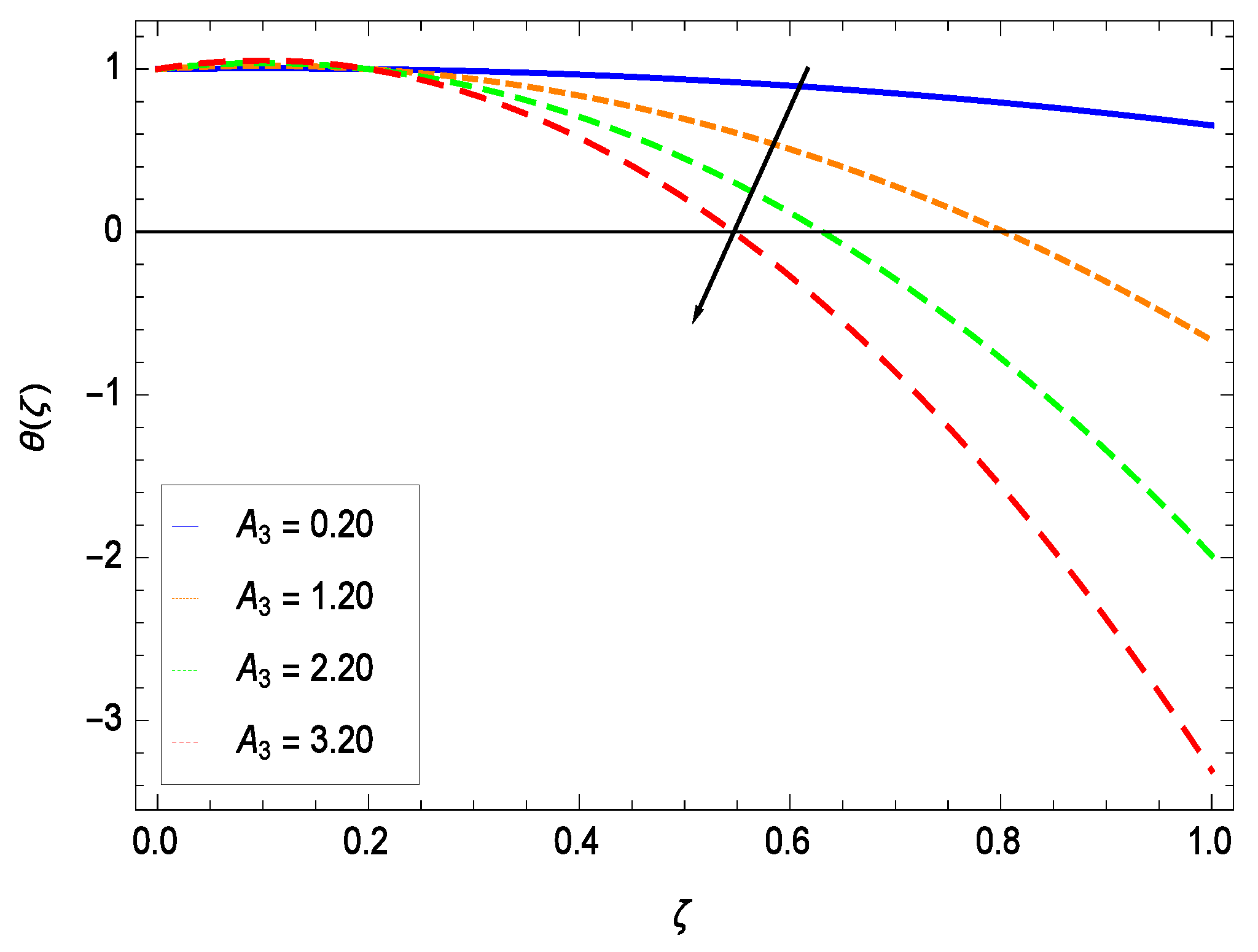
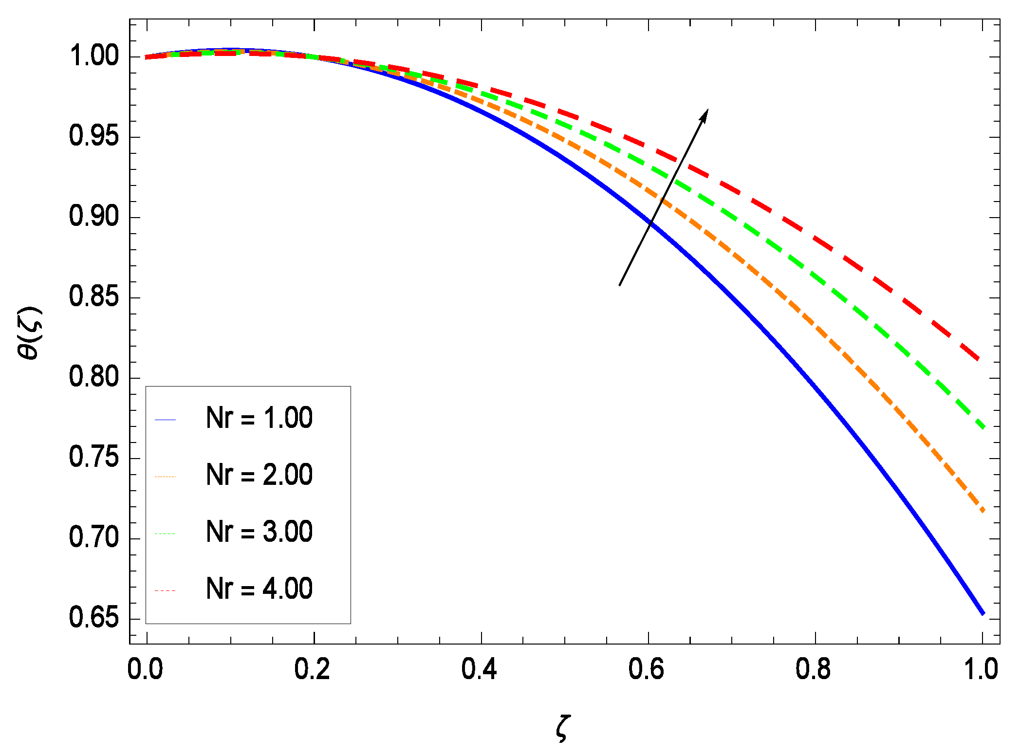
- The temperature () decreases with , S, n, We, and increasing A, and increases with , M and reducing A.
- (3)
- The skin friction coefficient f″(0) mitigates on elevating S and decreasing value of .
- (4)
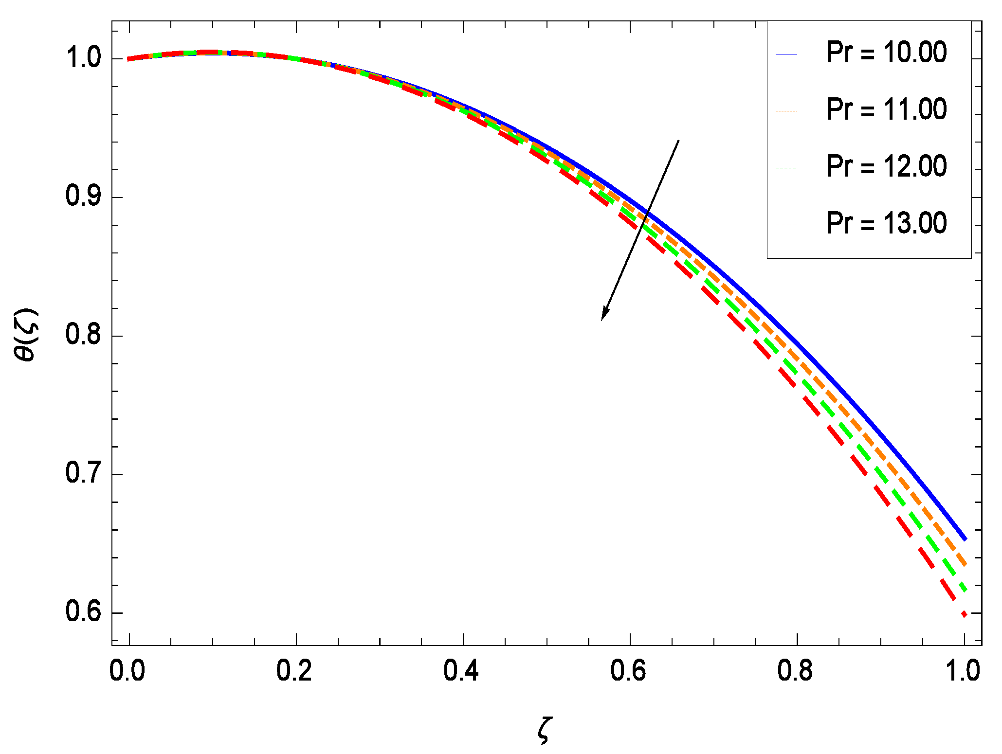
- The energy on surface () and energy gradient at wall (0) both decrease with increasing Prandtl number.
7. Future Work
Author Contributions
Funding
Acknowledgments
Conflicts of Interest
Nomenclature
| M | Magnetic field parameter |
| m | m-th order |
| n | Power law index |
| We | Weissenberg number |
| Nr | Thermal radiation parameter |
| Pr | Prandtl number |
| k | Thermal conductivity (m2 ) |
| k1 | Mean absorption coefficient |
| t | Time (s) |
| x | x-axis coordinate (m) |
| y | y-axis coordinate (m) |
| S | Unsteadiness parameter |
| and | Space and temperature dependent heat source/sink parameters respectively |
| u | Velocity component along x-axis (m ) |
| v | Velocity component along y-axis (m ) |
| Initial stretching velocity along x-axis (m ) | |
| V | Initial stretching velocity along y-axis (m ) |
| qr | Radiative heat flux (J ) |
| qw | Heat flux from the surface (J ) |
| c | Stretching rate () |
| Ci (i = 1–5) | Arbitrary constants |
| H(t) | Film size (m) |
| h | Auxiliary non-zero parameter |
| T | Temperature (K) |
| P | Pressure (kg ) |
| p | Embedding parameter ∈ [0, 1] |
| cp | Specific heat at constant pressure (J k ) |
| Surface temperature of the fluid (K) | |
| Initial temperature of the fluid (K) | |
| Reference temperature of the fluid (K) | |
| Wall temperature of the fluid (K) | |
| f | Dimensionless velocity |
| Initial guess | |
| Linear operator | |
| Linear operator | |
| Special solution | |
| Applied magnetic field strength | |
| Local dimensionless skin friction coefficient | |
| Local Nusselt number | |
| Local Reynolds number | |
| Greek symbols | |
| Volume fraction of the graphene nanoparticles | |
| (i = 1–5) | Nanofluid constants |
| Constant () | |
| Electrical conductivity | |
| Stefan-Boltzmann constant | |
| Physical stream function ( ) | |
| Dimensionless fluid thickness parameter | |
| Similarity variable | |
| Non-Newtonian time constant | |
| Square root of the half of the second invariant strain tensor | |
| Dimensionless temperature | |
| Initial guess | |
| Special solution | |
| ℵ | Non-linear operator |
| Kinematic viscosity ( ) | |
| Zero shear rate viscosity (kg ) | |
| ∏ | Second invariant strain tensor |
| Density (kg ) | |
| Shear stress at the surface (kg ) | |
| Subscripts | |
| s | Surface |
| sd | Solid nanoparticles |
| ref | Reference |
| w | Properties at the wall |
| nf | Nanofluid |
| f | Base fluid |
| o | Origin |
| x | Local value |
| Superscripts | |
| ′ | Differentiation with respect to |
References
- Khan, N.S.; Zuhra, S.; Shah, Z.; Bonyah, E.; Khan, W.; Islam, S. Slip flow of Eyring-Powell nanoliquid film containing graphene nanoparticles. AIP Adv. 2018, 8, 115302. [Google Scholar] [CrossRef]
- Sandeep, N.; Malvandi, A. Enhanced heat transfer in liquid film flow of non-Newtonian nanofluids embedded with graphene nanoparticles. Adv. Powder Technol. 2016, 27, 2448–2456. [Google Scholar] [CrossRef]
- Zuhra, S.; Khan, N.S.; Khan, M.A.; Islam, S.; Khan, W.; Bonyah, E. Flow and heat transfer in water based liquid film fluids dispensed with graphene nanoparticles. Results Phys. 2018, 8, 1143–1157. [Google Scholar] [CrossRef]
- Wu, P.; Qian, Y.; Du, P.; Zhang, H.; Cai, C. Facile synthesis of nitrogen-doped graphene for measuring the releasing process of hydrogen peroxide from living cells. J. Mater. Chem. 2012, 22, 6402–6412. [Google Scholar] [CrossRef]
- Yue, C.; Feng, J.; Feng, J.; Jiang, Y. Low thermal conductivity nitrogen-doped graphene aerogels for thermal insulation. RSC Adv. 2016, 6, 9396–9401. [Google Scholar] [CrossRef]
- Sadeghinezhad, E.; Meharali, M.; Latibari, S.T.; Meharali, M.; Kazi, S.N.; Oon, C.S.; Meselaar, H.S.C. Experimental investigation of convective heat transfer using graphene nanoplatelet based nanofluids under turbulent flow conditions. Ind. Eng. Chem. Res. 2014, 53, 12455–12465. [Google Scholar] [CrossRef]
- Guo, H.L.; Su, P.; Kang, X.; Ning, S.K. Synthesis and characterization of nitrogen-doped graphene hydrogels by hydrothermal rout with urea as reducing agents. J. Mater. Chem. A 2012. [Google Scholar] [CrossRef]
- Meharali, M.; Sadeghinezhad, E.; Latibari, S.T.; Meharali, M.; Togun, H.; Zubir, M.N.M.; Kazi, S.N.; Metselaar, H.S.C. Preparation, characterization, viscosity, and thermal conductivity of nitrogen-doped graphene aqueous nanofluids. J. Mater. Sci. 2014, 49, 7156–7171. [Google Scholar] [CrossRef]
- Meharali, M.; Sadeghinezhad, E.; Rashidi, M.M.; Akhiani, A.R.; Latibari, S.T.; Meharali, M.; Metselaar, H.S.C. Experimental and numerical investigation of the effective electrical conductivity of nitrogen-doped graphene nanofluids. J. Nanopart. Res. 2015, 17, 267. [Google Scholar] [CrossRef]
- Sheng, Z.H.; Shao, L.; Chen, J.J.; Bao, W.J.; Wang, F.B.; Xia, X.H. Catalyst-free synthesis of nitrogen-doped graphene via thermal annealing graphite oxide with melamine and its excellent electrocatalysis. ACS Nano 2011, 5, 4350–4358. [Google Scholar] [CrossRef] [PubMed]
- Reddy, A.L.M.; Srivastava, A.; Gowda, S.R.; Gullapalli, H.; Dubey, M.; Ajayan, P.M. Synthesis of nitrogen-doped graphene films for lithium battery application. ACS Nano 2010, 4, 6337–6342. [Google Scholar] [CrossRef] [PubMed]
- Khan, N.S.; Zuhra, Z.; Shah, Z.; Bonyah, E.; Khan, W.; Islam, S. Hall current and thermophoresis effects on magnetohydrodynamic mixed convective heat and mass transfer thin film flow. J. Phys. Commun. 2018. [Google Scholar] [CrossRef]
- Khan, N.S.; Gul, T.; Khan, M.A.; Bonyah, E.; Islam, S. Mixed convection in gravity-driven thin film non-Newtonian nanofluids flow with gyrotactic microorganisms. Results Phys. 2017, 7, 4033–4049. [Google Scholar] [CrossRef]
- Zuhra, S.; Khan, N.S.; Islam, S. Magnetohydrodynamic second grade nanofluid flow containing nanoparticles and gyrotactic microorganisms. Comput. Appl. Math. 2018, 37, 6332–6358. [Google Scholar] [CrossRef]
- Khan, N.S. Bioconvection in second grade nanofluid flow containing nanoparticles and gyrotactic microorganisms. Braz. J. Phys. 2018, 43, 227–241. [Google Scholar] [CrossRef]
- Palwasha, Z.; Islam, S.; Khan, N.S.; Ayaz, H. Non-Newtonian nanoliquids thin film flow through a porous medium with magnetotactic microorganisms. Appl. Nanosci. 2018, 8, 1523–1544. [Google Scholar] [CrossRef]
- Zuhra, S.; Khan, N.S.; Shah, Z.; Islam, S.; Bonyah, E. Simulation of bioconvection in the suspension of second grade nanofluid containing nanoparticles and gyrotactic microorganisms. AIP Adv. 2018, 8, 105210. [Google Scholar] [CrossRef]
- Khan, N.S.; Gul, T.; Islam, S.; Khan, W. Thermophoresis and thermal radiation with heat and mass transfer in a magnetohydrodynamic thin film second-grade fluid of variable properties past a stretching sheet. Eur. Phys. J. Plus 2017, 132. [Google Scholar] [CrossRef]
- Palwasha, Z.; Khan, N.S.; Shah, Z.; Islam, S.; Bonyah, E. Study of two-dimensional boundary layer thin film fluid flow with variable thermophysical properties in three dimensions space. AIP Adv. 2018, 8, 105318. [Google Scholar] [CrossRef]
- Khan, N.S.; Gul, T.; Islam, S.; Khan, I.; Alqahtani, A.M.; Alshomrani, A.S. Magnetohydrodynamic nanoliquid thin film sprayed on a stretching cylinder with heat transfer. J. Appl. Sci. 2017, 7, 271. [Google Scholar] [CrossRef]
- Khan, N.S.; Gul, T.; Islam, S.; Khan, A.; Shah, Z. Brownian motion and thermophoresis effects on MHD mixed convective thin film second-grade nanofluid flow with Hall effect and heat transfer past a stretching sheet. J. Nanofluids 2017, 6, 812–829. [Google Scholar] [CrossRef]
- Khan, N.S.; Gul, T.; Islam, S.; Khan, W.; Khan, I.; Ali, L. Thin film flow of a second-grade fluid in a porous medium past a stretching sheet with heat transfer. Alex. Eng. J. 2017. [Google Scholar] [CrossRef]
- Khan, N.S.; Shah, Z.; Islam, S.; Khan, I.; Alkanhal, T.A.; Tlili, I. Entropy generation in MHD mixed convection non-Newtonian second-grade nanoliquid thin film flow through a porous medium with chemical reaction and stratification. Entropy 2019, 21, 139. [Google Scholar] [CrossRef]
- Khan, N.S.; Zuhra, S.; Shah, Q. Entropy generation in two phase model for simulating flow and heat transfer of carbon nanotubes between rotating stretchable disks with cubic autocatalysis chemical reaction. Appl. Nanosci. 2019. [Google Scholar] [CrossRef]
- Sulochana, C.; Ashwinkumar, G.P. Carreau model for liquid thin film flow of dissipative magnetic-nanofluids over a stretching sheet. Int. J. Inf. Technol. 2017, 10, 239–254. [Google Scholar] [CrossRef]
- Raju, C.S.K.; Hoque, M.M.; Khan, N.A.; Islam, M.; Kumar, S. Multiple slip effects on magnetic-Carreau fluid in a suspension of gyrotactic microorganisms over a slendering sheet. Proc. Inst. Mech. Eng. Part E J. Process Mech. Eng. 2018. [Google Scholar] [CrossRef]
- Irfan, M.; Khan, W.A.; Khan, M.; Gulzar, M.M. Influence of Arrhenius energy in chemically reactive radiative flow of 3D Carreau nanofluid with nonlinear mixed convection. J. Phys. Chem. Solids 2019, 125, 141–152. [Google Scholar] [CrossRef]
- Waqas, M.; Khan, M.I.; Hayat, T.; Alsaedi, A. Numerical simulation for magneto Carreau nanofluid model with thermal radiation: A revised model. Comput. Methods Appl. Mech. Eng. 2017, 324, 640–653. [Google Scholar] [CrossRef]
- Mahmoud, M.A.A.; Megahed, A.M. Slip flow of Powell-Eyring liquid film due to an unsteady stretching sheet with heat transfer generation. Braz. J. Phys. 2016. [Google Scholar] [CrossRef]
- Liao, S.J. Homotopy Analysis Method in Non-Linear Differential Equations; Higher Education Press: Beijing, China; Springer: Berlin/Heidelberg, Germany, 2012. [Google Scholar]


| Aspects | Pure Water | Graphene |
|---|---|---|
| (kg/m3) | 997 | 2250 |
| (J/kg K) | 4076 | 2100 |
| k (W/m K) | 0.605 | 2500 |
| (Ωm | 0.005 | 1 × |
| Parameter | Mahmoud and Megahed [29] | Present Results | ||
|---|---|---|---|---|
| S | −(0) | −(0) | ||
| 0.4 | 4.981455 | 1.134096 | 4.981455 | 1.134095 |
| 0.6 | 3.131711 | 1.195125 | 3.131711 | 1.195123 |
| 0.8 | 2.151992 | 1.245805 | 2.151992 | 1.245803 |
| 1.0 | 1.543616 | 1.277769 | 1.543616 | 1.277768 |
| 1.2 | 1.127781 | 1.279171 | 1.127781 | 1.279173 |
| 1.4 | 0.821032 | 1.233545 | 0.821032 | 1.233546 |
| 1.6 | 0.576175 | 1.114939 | 0.576175 | 1.114938 |
| 1.8 | 0.356389 | 0.867416 | 0.356389 | 0.867415 |
| Parameters | Mahmoud and Megahed [29] | Present Results | ||||
|---|---|---|---|---|---|---|
| Pr | S | () | (0) | () | (0) | |
| 0.01 | 0.8 | 2.151990 | 0.960440 | 0.042023 | 0.960441 | 0.042024 |
| 0.1 | 0.8 | 2.151990 | 0.692268 | 0.351319 | 0.692265 | 0.351318 |
| 1.0 | 0.8 | 2.151990 | 0.097825 | 1.671917 | 0.097823 | 1.671915 |
| 2.0 | 0.8 | 2.151990 | 0.024868 | 2.443816 | 0.024864 | 2.443815 |
| 3.0 | 0.8 | 2.151990 | 0.008325 | 3.036115 | 0.008324 | 3.036113 |
| 0.01 | 1.2 | 1.127780 | 0.982311 | 0.033417 | 0.982312 | 0.033418 |
| 0.1 | 1.2 | 1.127780 | 0.843485 | 0.305406 | 0.843484 | 0.305407 |
| 1.0 | 1.2 | 1.127780 | 2.86635 | 1.773774 | 2.86634 | 1.773775 |
| 2.0 | 1.2 | 1.127780 | 0.128174 | 2.638433 | 0.128173 | 2.638435 |
| 3.0 | 1.2 | 1.127780 | 0.067738 | 3.280327 | 0.067739 | 3.280325 |
© 2019 by the authors. Licensee MDPI, Basel, Switzerland. This article is an open access article distributed under the terms and conditions of the Creative Commons Attribution (CC BY) license (http://creativecommons.org/licenses/by/4.0/).
Share and Cite
Khan, N.S.; Gul, T.; Kumam, P.; Shah, Z.; Islam, S.; Khan, W.; Zuhra, S.; Sohail, A. Influence of Inclined Magnetic Field on Carreau Nanoliquid Thin Film Flow and Heat Transfer with Graphene Nanoparticles. Energies 2019, 12, 1459. https://doi.org/10.3390/en12081459
Khan NS, Gul T, Kumam P, Shah Z, Islam S, Khan W, Zuhra S, Sohail A. Influence of Inclined Magnetic Field on Carreau Nanoliquid Thin Film Flow and Heat Transfer with Graphene Nanoparticles. Energies. 2019; 12(8):1459. https://doi.org/10.3390/en12081459
Chicago/Turabian StyleKhan, Noor Saeed, Taza Gul, Poom Kumam, Zahir Shah, Saeed Islam, Waris Khan, Samina Zuhra, and Arif Sohail. 2019. "Influence of Inclined Magnetic Field on Carreau Nanoliquid Thin Film Flow and Heat Transfer with Graphene Nanoparticles" Energies 12, no. 8: 1459. https://doi.org/10.3390/en12081459