A Heuristic Home Electric Energy Management System Considering Renewable Energy Availability

Abstract

This paper presents the development of a heuristic-based algorithm for a Home Electric Energy Management System (HEEMS). The novelty of the proposal resides in the fact that solutions of the Pareto front, minimizing both the energy consumption and cost, are obtained by a Genetic Algorithm (GA) considering the renewable energy availability as well as the user activity level (AL) inside the house. The extensive solutions search characteristic of the GAs is seized to avoid the calculation of the full set of Pareto front solutions, i.e., from a reduced set of non-dominated solutions in the Pareto sense, an optimal solution with the best fitness is obtained, reducing considerably the computational time. The HEEMS considers models of the air conditioner, clothes dryer, dishwasher, electric stove, pool pump, and washing machine. Models of the wind turbine and solar PV modules are also included. The wind turbine model is written in terms of the generated active power exclusively dependent on the incoming wind profiles. The solar PV modules model accounts for environmental factors such as ambient temperature changes and irradiance profiles. The effect of the energy storage unit on the energy consumption and costs is evaluated adapting a model of the device considering its charge and discharge ramp rates. The proposed algorithm is implemented in the Matlab^® platform and its validation is performed by comparing its results to those obtained by a freeware tool developed for the energy management of smart residential loads. Also, the evaluation of the performance of the proposed HEEMS is carried out by comparing its results to those obtained when the multi-objective optimization problem is solved considering weights assigned to each objective function. Results showed that considerable savings are obtained at reduced computational times. Furthermore, with the calculation of only one solution, the end-user interaction is reduced making the HEEMS even more manageable than previously proposed approaches.

1. Introduction

During the last decade, the development of smart grids (SGs) has increased exponentially empowered by the benefits of renewable energy resources [1]. Control and optimization strategies, together with communication systems integrated to the conventional electrical distribution systems, represent the cornerstone for the adoption of the SG concept [2]. One of the new desired functionalities and requirements of SG is the implementation of demand-side management programs such as Demand Response (DR), which basically consist of the incorporation of distribution system automation techniques for load control, allowing the reduction of energy consumption during critical operating times. This benefits not only the final user, by reducing its energy costs, but also the Local Distribution Companies (LDCs), by reducing the peak load, reshaping load profiles, and increasing system sustainability [3]. Furthermore, an additional indirect benefit of DR programs is the deferral of investments in both the transmission and distribution systems expansion and the construction of new generating plants.

DR allows end users to actively participate in the electricity markets by offering their load reductions in response to signals sent by the LDCs requesting load management. Traditionally, these requests were focused on the industrial and commercial sectors because of the magnitude of their loads; nevertheless, owing to the full deployment of the advanced metering infrastructure in some countries, residential users have emerged as new DR service providers and the LCDs are now searching for new tools, programs, or incentives to increase their responsiveness. The main challenge at this point is to develop “smart” control devices, deployed at the residential end-user premises, with embedded software capable of receiving, interpreting, and analyzing different types of input signals with the purpose of performing appropriate control actions over a set of predefined controllable loads, requiring little or no human intervention. These devices, commonly termed to as energy management systems or Home Energy Management Systems (HEMS), must be able to produce win-win scenarios for both the end users and the LDCs in terms of cost, comfort, and system reliability. However, there are important factors that must be considered: (1) electricity prices are not the only drivers affecting DR participation rates, e.g., residential customers do not want to spend time acquiring the necessary expertise to analyze consumption patterns and control decisions to micromanage household devices to save money [4]; (2) the HEMS are time-restricted for producing the necessary operational decisions; (3) the on-site renewable energy availability; (4) the users preferences and their activity inside the house; etc.

In this context, several approaches have proposed the development of a variety of such devices embedding a diversity of control strategies for load management. A useful and comprehensive review of the modeling approaches and the complexity of previously proposed HEMS is presented in [5]. Emphasis is given to the most important factors that influence HEMS operations and outcomes such as tariff structure offered by the LCDs, controllable devices, uncertainties, multi-objective nature and the associated solution methods, on-site renewable energy generation (PV/Wind), and battery/energy storage devices. Similarly, the significance of embedding renewables into HEMS is exposed in [6] when analyzing the trends of the development of renewable residential resources and the satisfactory results that have been reported, motivating the continuous research in this field. For instance, a model for cost minimization considering the price to sell local generation energy, models of appliances, and a thermal model of the house is presented in [7]. Results reported highlight the advantages of the on-site generation. The economics of providing peak shaving with DR using various storage technologies is evaluated in [8]. Based on the favorable results in all cases, it is shown how end users will significantly benefit when installing storage devices to shave load peaks under a Time-of-Use (TOU) tariff scenario.

It is noted in [5] that most of the optimization problems associated with HEMS have been solved using traditional optimization algorithms such as linear programming, non-linear programming, and dynamic programming. However, their drawbacks when dealing with ON/OFF decisions (integer variables) have generated a demand for other types of algorithms such as heuristic optimization approaches [5,9]. Examples of approaches applying these types of optimization approaches are given in [10,11], where two HEMS reducing the energy costs and peak demand are proposed. The former proposes an algorithm where the household appliances are modeled by their energy consumption level only; the latter proposes a binary backtracking search algorithm for the optimal dispatch of the heating, ventilation, and air conditioning system (HVAC), water heater, refrigerator, smart outlets, and washing machine. However, no results about solution times are reported in these proposals, which is an important factor to be considered since heuristic algorithms may take too long to converge to a solution or even may diverge. Furthermore, based on the multi-objective nature of the optimization problems associated with the HEMS, there could exist several solutions satisfying the objective functions and the final user should select the best one based on its preferences and needs, even though end users may not want to spend time selecting the appropriate solution over a vast set of solutions. For this reason, some approaches have proposed to reduce the set of solutions by obtaining the Pareto front of solutions associated with the multi-objective optimization problem making the controller easier to manage. For instance, Pareto front algorithms to optimally schedule the energy consumption are developed in [12,13]. However, the first algorithm is designed for energy management entities with high computing capabilities because of the high computational times reported, and the second does not consider explicit models of the renewable energy generation units, making not possible to evaluate the energy availability in the household.

The Non-dominated Sorting Genetic Algorithm II (NSGA-II) is applied in [14,15] to generate more economic usage profiles for controllable appliances. A drawback of the former is that it cannot be applied to household appliances with fixed operating times, limiting its applicability, whereas the latter does not consider renewable energy generation and uses simplistic models of the household appliances. The NSGA-II algorithm is also used in [16], where a set of microgrids sent their corresponding load curve to an operating center for flattening purposes, then, dynamic appliance scheduling was carried out by sequentially solving two optimization problems: one for the non-flexible loads and one for the flexible loads; a Pareto front is generated based on the minimization of a load flattening function and the delay to supply the household appliances; a PV generation is also considered using a simplified model of negative load power. Just recently, fuzzy logic combined with optimization techniques and supervisory control strategies have been applied for cost, energy consumption, and peak-to-average ratio reduction [17,18]. However, they do not account for the renewable energy generation. Also, preliminary results of the parallelization of a control algorithm is presented in [19]. Finally, it is emphasized in [20] that the HEMS incorporation with transactive energy controls would improve the performance and efficiency of these systems, a topic which is currently being addressed by several researchers around the world.

From this review, it can be noticed that few approaches consider the determination of a Pareto front of solutions of the multi-objective problem associated with the HEMS. Even more important, none of them determine the Pareto front considering the renewable energy availability, the user preferences, and its activity inside the house, which has a direct impact on the energy consumption, to optimally dispatch the set of household appliances. Furthermore, the resulting Pareto set may contain a variety of solutions that still require the selection of the end user. For these reasons, the scope of this proposal is the development of a heuristic-based algorithm for the optimal management of the electric energy. The novelty of the proposed algorithm called Home Electric Energy Management System (HEEMS) resides in the fact that solutions of the Pareto front, minimizing the energy consumption and cost, are obtained by a Genetic Algorithm (GA) considering both the renewable energy availability (including batteries as energy storage device) and an index proposed in [21] for the user activity level (AL) inside the house, representing an advantage over previously proposed approaches. The extensive solutions search characteristic of the GAs is exploited to select an optimal solution with the best fitness from a set of non-dominated solutions in the sense of Pareto, i.e., at each iteration of the GA, Pareto front solutions are obtained and a solution with the best fitness is added to a reduced set of solutions; once iterations have finished, a new Pareto test and fitness evaluation is performed to the reduced set of solutions to obtain the best solution, reducing to one the number of solutions available to the user, and as consequence the computational time, which are two of the main goals of the proposal. Moreover, the proposed approach takes advantage of the good results reported in [21,22] to adapt the models of the household appliances, PV/wind energy generation and energy storage units (batteries).

It is important to mention that this work is limited to the electric energy management considering a set of the most common household devices and two types of renewable energy generation units. However, and as will be pointed out in the next sections, other types of devices can be considered without affecting the performance of the algorithm. Even though the energy availability is considered when dispatching the electric loads, the sale of surplus energy is not considered. Finally, an overall cost analysis including a variety of factors such as optimal sizing of the system´s components, components’ lifespan and cost, manufacturers, and deployment and maintenance costs is not the objective of this proposal. Instead, evaluations of savings are considered on a daily basis.

The rest of the paper is organized as follows: Section 2 presents the optimization model, models of the main household devices, and renewable energy generation and storage units, which constitute the operational constraints. Additionally, the end-user AL is also described in that section. The GA used to solve the multi-objective optimization problem is presented in Section 3. Results of the experimental test are discussed in Section 4. Finally, the main conclusions and contributions of this research are highlighted in Section 5.

2. Optimization Model

The nomenclature used to formulate the proposed optimization model, such as indices, sets, subscripts, and variables are defined in

Table 1. Indices, sets, subscripts, and variables used in the proposed optimization model.

Indices	Name	Subscripts	Name
i	Index of devices	pp	Pool pump
k	Number of iterations	pv	Solar PV panel
t	Time interval index	st	Energy storage unit
Sets		wm	Washing machine
A	Set of devices	wt	Wind turbine
T	Scheduling horizon	Variables
Ti	Set of periods in which device i may operate	f1	Energy consumption objective function
Subscripts		f2	Energy cost objective function
ac	HVAC cooling mode	Pi(t)	Power of device i ∈ A = pv, st, wt [kW]
cd	Clothes dryer	Q	New individual resulting from GA
char	Charging mode	Schar/dis(t)	Charge/discharge modes of device st at interval t
dis	Discharging mode	Sφ	Fittest set of solutions
dw	Dishwasher	Si(t)	ON/OFF state of device i at interval t
es	Electric stove	θin(t)	Temperature inside the house at interval t [°C]
ht	HVAC heating mode

, whereas the set of parameters is defined in

Table 2. Parameters used in the proposed optimization model.

Parameters
Area	Area of PV modules [m2]	Pdcons(t)	Active power load surplus at interval t [kW]
a, b, c	Parameters of the quadratic equation defining the output power of the wind turbine	Pdg(t)	Aggregated renewable power generation surplus at interval t [kW]
AL(t)	Activity level index at interval t	Pg(t)	Power generated by renewables (Ppv(t) + Pwt(t)) at interval t [kW]
αac/ht	Cooling/Warming effect of an ON state of the HVAC on the corresponding variable	Pi(t)	Power of device i ∈ A ≠ pv, st, wt at time interval t [kW]
βac/ht	Cooling/Warming effect of an OFF state of the HVAC on the corresponding variable	Pmax/min	Maximum/minimum real power [kW]
c(t)	Electricity price at interval t	Pmut	Mutation probability
δ	Self-discharge factor of battery	Prat	Rated power [kW]
di	Device i ∈ A ≠ pv, st, wt, ac, ht operative cycle	Prc	Active power charge rate
φ(t)	Solar irradiation [kW/m2]	Prd	Active power discharge rate
η	Energy conversion efficiency	ρac/ht	Effect of inside and outside temperature difference on the inside temperature
ηc	Rectifier efficiency	ti,end	Latest operation time of device i
ηd	Inverter efficiency	${\theta }_{in}^{max}$	Upper limit of the temperature inside the house
N	Number of individuals in the population	${\theta }_{in}^{min}$	Lower limit of the temperature inside the house
Npv	Number of PV modules	ti,start	Earliest operation time of device i
P	GA population	θamb(t)	Ambient temperature at interval t [°C]
P′	New GA population	v(t)	Wind speed velocity [m/s]
Pc(t)	Active power in charging mode at time interval t [kW]	Vci	Cut-in wind speed [m/s]
Pcons(t)	Power consumed by the household loads at interval t [kW]	Vco	Cut-out wind speed [m/s]
Pcross	Cross probability	Vr	Rated wind speed [m/s]
Pd(t)	Active power in the discharge mode at interval t [kW]

.

The optimization model proposed in this paper minimizes both the energy consumption and costs by optimally scheduling the household appliances, considering the energy availability generated by the on-site renewable resources, subject to devices’ operational constraints. The general form of the multi-objective optimization model may be written as follows:

$$\begin{array}{l}\min \left[f_1,f_2\right]\\ \mathrm{s}.\mathrm{t}.\mathrm{Device}i\mathrm{operational}\mathrm{constraints}\forall i\in A\end{array},$$

(1)

where f₁ and f₂ stand for the energy consumption and costs functions, respectively, and are defined by:

$$f_1={\displaystyle \sum _{t\in T}\left[\underset{loads}{\underbrace{{\displaystyle \sum _{\begin{array}{l}i\in A\\ A\notin \left\{wt,pv,st\right\}\end{array}}{S}_i\left(t\right)P_i\left(t\right)}}}-\underset{renewablesandstorageunits}{\underbrace{{\displaystyle \sum _{A\in \left\{wt,pv,st\right\}}{S}_i\left(t\right)P_i\left(t\right)}}}\right]},$$

(2)

$$f_2={\displaystyle \sum _{t\in T}c\left(t\right)}\left[\underset{loads}{\underbrace{{\displaystyle \sum _{\begin{array}{l}i\in A\\ A\notin \left\{wt,pv,st\right\}\end{array}}{S}_i\left(t\right)P_i\left(t\right)}}}-\underset{renewablesandstorageunits}{\underbrace{{\displaystyle \sum _{A\in \left\{wt,pv,st\right\}}{S}_i\left(t\right)P_i\left(t\right)}}}\right],$$

(3)

This model is solved by a GA with the purpose to obtain solutions of the Pareto front and then select the one with the best fitness, as explained in the next section. The traditional scheduling horizon T considered in optimization models for load management in the residential sector is used in this work and is set to 24 h [5].

2.1. Devices’ Operational Constraints

The load scheduling must consider the devices’ operational constraints and user preferences. Furthermore, when considering on-site renewable generation units, the generated power should be optimally managed to exploit their benefits and to reduce energy waste. The operative constraints of devices whose operating mode is defined by operative windows such as cd, dw, es, pp, and wm are formulated as:

$$S_i\left(t\right)=\{\begin{array}{l}0\mathrm{or}1\mathrm{if}t\in T_i\\ 0\mathrm{if}t\notin T_i\end{array}\forall i\in A\ne pv,st,wt,$$

(4)

$$t_{i,start}\le T_i\le t_{i,end}\forall i\in A\ne pv,st,wt,ac,ht,$$

(5)

$${\displaystyle \sum _{k=t}^{t+d_i}{S}_i\left(k\right)=}{d}_i\begin{array}{c}\forall i\in A\ne pv,st,wt,ac,ht\\ \forall t\in T_i\end{array},$$

(6)

Equation (4) specifies the ON/OFF decisions of device i according to the time during which it may operate, Equation (5) defines the scheduling window where the user considers the device’s task should be finished, and Equation (6) enforces the operative cycle d_i is met as defined by the user. It is worth noting that t_i,start, t_i,end, and d_i are specified by the user according to its needs, e.g., a user may desire to have its clothes clean at 6:00 a.m. when put the load at 12:00 a.m. selecting one washing cycle of one hour, for this case t_i,start = 0, t_i,end = 6, and d_i =1 over a time horizon of 24 h. In this way, the optimization model will try to optimally move the operating cycle d_i of one hour of duration over a 6 hours window to minimize energy costs. Note that for these appliances, the energy consumption will not change since they are requested to operate for fixed time periods, opposite to the case of the HVAC system where the operation intervals will depend on thermal interactions of the air masses inside the house.

2.1.1. Heating, Ventilation, and Air Conditioning System

One of the devices consuming the major energy within a house is the HVAC system. For this reason, proper management of its demand will produce important energy and cost savings. However, an important factor that must be considered for the successful management of the device is the end-user comfort. In this paper, the HVAC model proposed in [21] is used since considers factors such as indoor and outdoor temperatures, thermal characteristics of the house, as well as the end-user AL represented by an index. The model is defined as:

$$S_i\left(t\right)=\{\begin{array}{lll}1& \mathrm{if}{\theta }_{in}\left(t-1\right)>{\theta }_{in}^{\max }& i=ac\\ 0& \mathrm{if}{\theta }_{in}\left(t-1\right)<{\theta }_{in}^{\min }& \end{array},$$

(7)

$$S_i\left(t\right)=\{\begin{array}{lll}1& \mathrm{if}{\theta }_{in}\left(t-1\right)<{\theta }_{in}^{\min }& i=ht\\ 0& \mathrm{if}{\theta }_{in}\left(t-1\right)>{\theta }_{in}^{\max }& \end{array},$$

(8)

$${\theta }_{in}^{\min }\left(t\right)\le {\theta }_{in}\left(t\right)\le {\theta }_{in}^{\max }\left(t\right)\forall t\in T_i,i\in \left\{ac,ht\right\},$$

(9)

$$S_{ac}\left(t\right)+S_{ht}\left(t\right)\le 1\forall t\in T_i,$$

(10)

$${\theta }_{in}\left(t\right)={\theta }_{in}\left(t-1\right)+\mathsf{\Delta }t\left[{\beta }_{ac}AL\left(t\right)-{\alpha }_{ac}{S}_i\left(t\right)+{\rho }_{ac}\left({\theta }_{amb}\left(t\right)-{\theta }_{in}\left(t\right)\right)\right]\forall t\in T,i=ac,$$

(11)

$${\theta }_{in}\left(t\right)={\theta }_{in}\left(t-1\right)+\mathsf{\Delta }t\left[{\beta }_{ht}AL\left(t\right)+{\alpha }_{ht}{S}_i\left(t\right)+{\rho }_{ht}\left({\theta }_{amb}\left(t\right)-{\theta }_{in}\left(t\right)\right)\right]\forall t\in T,i=ht,$$

(12)

Equation (4) ensures the HVAC system is in operation for the time interval defined by the user, although in this paper is considered an operation interval of 24 h, this equation allows the user to operate the device according to its preferences; Equations (7)–(9) turn the device ON/OFF when the temperature is outside/inside the predefined limits; equation (10) is defined to ensure that the air conditioner and furnace do not operate simultaneously; Equations (11) and (12) drive the indoor temperature. α_ac/ht represents the thermal effect of an ON state of the HVAC system on the indoor temperature, β_ac/ht accounts for the effect of the AL on the indoor temperature increase, and ρ_ac/ht represents the net effect of heat transfer between the outdoor and indoor temperatures differences. Calculation of these parameters is described in [23]. Details about the AL calculation are given in the next subsection. It is worth noting that to consider other devices with thermal energy storage capacity such as fridge, water heater, and hot tub water heater, the same set of constraints defined by Equations (7)–(12) can be used since these devices should maintain their respective temperatures within user-specified ranges, i.e. Equations (7)–(11) are used for the case of the fridge and Equations (7)–(10) and (12) are used for the case of the water heater and the hot tub water heater. The only difference between these models is in their parameter settings such as average hot water usage, temperature settings, operational time, and associated coefficients that may have different values [21,24].

Equations (11) and (12) are used to calculate parameters α_ac/ht, β_ac/ht, and ρ_ac/ht as follows: given as inputs measurements of the inside temperature (θ_in,meas), the status of the i-th device (S_i(t)), ambient temperature, and the AL, the following least square absolute error minimization problem is solved:

$$\begin{array}{l}\min \left({\theta }_{in,meas}-{\theta }_{in,calc}\right)\\ s.t.{\theta }_{in,calc}\left(t\right)={\theta }_{in,calc}\left(t-1\right)+\\ +\mathsf{\Delta }t\left[{\beta }_{i}AL\left(t\right)-{\alpha }_i{S}_i\left(t\right)+{\rho }_i\left({\theta }_{amb}\left(t\right)-{\theta }_{in,meas}\left(t\right)\right)\right]\begin{array}{c}\forall t\in T\\ i=ac,ht\end{array}\end{array},$$

(13)

As a result, the associated parameters are adjusted minimizing deviations between calculated and measured values of the inside temperature.

2.1.2. Wind Turbine

A simplified wind turbine model proposed in [22] is adopted in the present work. The model focuses on the operative behavior of the wind turbine in terms of the generated active power exclusively dependent on the incoming wind profiles. The model is written as:

$$P_{wt}\left(t\right)=\{\begin{array}{cc}0& \mathrm{if}v\left(t\right)<V_{ci}orv\left(t\right)>V_{co}\\ \left(a+bv\left(t\right)+cv{\left(t\right)}^2\right)P_{rat}& \mathrm{if}{V}_{ci}\le v\left(t\right)<V_r\\ P_{rat}& \mathrm{if}{V}_r\le v\left(t\right)\le V_{co}.\end{array},$$

(14)

Three operative conditions are defined in Equation (14): the first condition suppresses the power output of the wind turbine when the wind speed is above or below of the cut out and cut in wind speeds, respectively; the second condition defines the output power as a quadratic equation describing the behavior of the wind turbine when the wind speed is into operative values, values of a, b and c are calculated as shown in [25]; the third condition set the maximum power contribution of the device when the wind speed is between rated and maximum values.

2.1.3. Solar PV Panel

A model of the solar PV panel proposed in [26] is implemented in this proposal. It accounts for environmental factors such as ambient temperature changes and irradiance profiles. The model is written as:

$$P_{pv}\left(t\right)=\eta \cdot Area\cdot N_{pv}\cdot \varphi \left(t\right)\cdot \left[1-0.005\left({\theta }_{amb}\left(t\right)+25\right)\right],$$

(15)

The model considers losses due to the temperature of the panel taking 25 °C as a base temperature.

2.1.4. Energy Storage Unit

The inclusion of storage units arises from the need to take full advantage of the renewable energy resources installed in the house allowing more energy independence. To properly model the operative behavior of this device, two scenarios need to be considered: the first scenario is when the house load level is lower than the energy produced by renewables such that the energy is not fully exploited and is supplied to the electric distribution system; the second scenario is the opposite case, the surplus demand needs to be fed with energy coming from the distribution system. In the former case, if energy storage units are available, the surplus energy generated by renewables is stored to be used when necessary; in the latter case, instead of drawing energy from the grid, energy storage units are used to feed the surplus load. A model for the energy storage unit considering not only these scenarios but also its self-discharge characteristic and efficiencies of the inverter and rectifier is proposed in [22]. This model has been adapted in terms of active power to be properly considered in the objective functions defined by Equations (2) and (3). Furthermore, constraints regarding the charge and discharge states have been included to account for the energy availability produced by the renewable generation units. The model, written by all t ∈ T, is described by the following equations:

$$S_{char}\left(t\right)=\{\begin{array}{cc}1& \mathrm{if}{P}_g\left(t\right)>P_{cons}\left(t\right)\\ 0& \mathrm{if}{P}_g\left(t\right)<P_{cons}\left(t\right)\end{array},$$

(16)

$$S_{dis}\left(t\right)=\{\begin{array}{cc}1& \mathrm{if}{P}_g\left(t\right)<P_{cons}\left(t\right)\\ 0& \mathrm{if}{P}_g\left(t\right)>P_{cons}\left(t\right)\end{array},$$

(17)

$$P_{\min }\le P_{st}\left(t\right)\le P_{\max },$$

(18)

$$S_{char}\left(t\right)+S_{dis}\left(t\right)\le 1,$$

(19)

$$P_c\left(t\right)=\min \left(P_{rc},P_{dg}\left(t\right)\right),$$

(20)

$$P_d\left(t\right)=\min \left(P_{rd},P_{dcons}\left(t\right)\right),$$

(21)

$$P_{st}\left(t+1\right)=P_{st}\left(t\right)\left(1-\delta \right)+{\eta }_c{P}_c\left(t\right)S_{char}\left(t\right)-\frac{P_d\left(t\right)}{{\eta }_d}{S}_{dis}\left(t\right),$$

(22)

Equations (16) and (17) set the charge/discharge modes when the power consumed by the household loads is lower/higher than the power generated by the renewable generation units; Equation (18) maintains the power of the unit between prespecified limits; Equation (19) guarantees the charge and discharge modes are not simultaneously activated; Equations (20) and (21) account for the unit capacity to charge and discharge; finally, Equation (22) represents the active power of the unit at interval t + 1. It is important to mention that the multi-objective nature of GAs allows the inclusion of new objective functions and constraints without modifying the algorithm structure. For instance, cost functions associated with the lifespan of the household devices and system components could be considered as objective functions, as well as new operative constraints that could result from a refinement of the household devices operation.

2.2. End-User Activity Level

Since the household occupancy and activity inside a house depend on the hour of the day, the day of the week, and the season of the year, they have a major impact on the energy consumption. For this reason, it is necessary to have a measure of such an activity in order to be included to some of the appliance models to reflect the human activity in the devices’ operation patterns. To consider the effect of household occupancy on energy consumption patterns, an index termed to as AL proposed in [21,24] is used. This index is a normalized value of the ratio between the energy consumed at each interval and the total energy consumption of the day. It uses historical measurements of energy consumption patterns provided by smart meters installed in each house. The good results showed have motivated authors to use this index to account for the human activity inside a house. Details of its calculation are provided in [21,24].

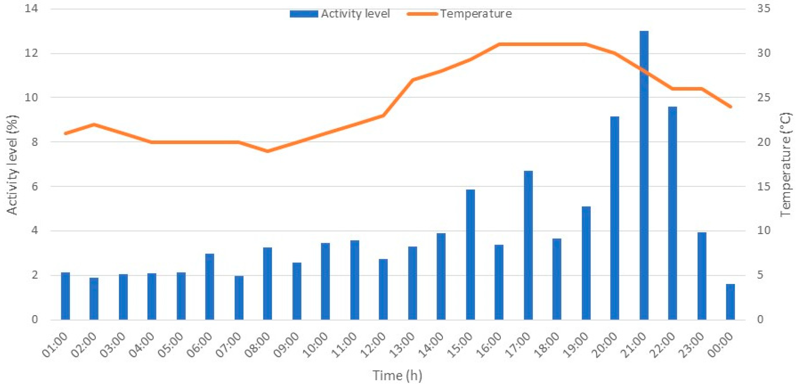
An electricity consumption and occupancy data set available at [27] was used to obtain the AL values used in the simulations presented in this work. The open-source data set for load monitoring and occupancy detection research was collected in six Swiss pilot houses over a period of eight months, containing measurements of the main electrical parameters and occupancy inside each house at time intervals of 1 s. An example of the AL calculated of one of the houses for the hottest day of summer of 2012 is presented in Figure 1. Temperature profiles were obtained from [28].

In this figure, the AL is normalized w.r.t. the total energy consumption of the day, which is assumed to be 100%. The AL is included in the model of the HVAC as described in the previous subsection.

3. Multi-Objective Genetic Algorithm

GAs, well-known techniques for solving a wide type of optimization problems, are search algorithms imitating the biological processes of reproduction and natural selection [29]. Have shown wide applicability to successfully solve mixed-integer linear and nonlinear optimization problems. In general terms, a GA takes an initial population containing a number of individuals, each representing a possible solution to the optimization problem, encoded by a particular genotype or chromosome; each individual is evaluated by a fitness function to determine its performance or phenotype. On the basis of this evaluation, the population is subjected to a selection mechanism, which takes a group of individuals to be the origin of a new population where, just as in nature, natural selection is the determining factor of which individuals are the aptest to evolve. A key part of GAs is the implementation of two basic operators: sexual recombination or crossing and mutation. The crossing operator consists of taking a pair of individuals to form a new one, where its chromosome will contain parts of each selected parent chromosomes. The mutation operator establishes a probability for the modification of a chromosome, allowing the introduction of new solutions to the population under study. The introduction of these operators allows the generation of a new population that can partially or completely replace the previous generation, depending on certain policies of elitism. It is worth noting that in the context of this work, each chromosome is composed of individual structures called genes, where each gen is a binary string representing the activation status (ON/OFF decisions) of all devices at time t. Hence, a chromosome will have as many genes as time intervals considered in the scheduling horizon. Generally, the stopping criteria established for GAs is based on the maximum number of iterations under the premise that, after several cycles of evolution, the population must contain the fittest individuals.

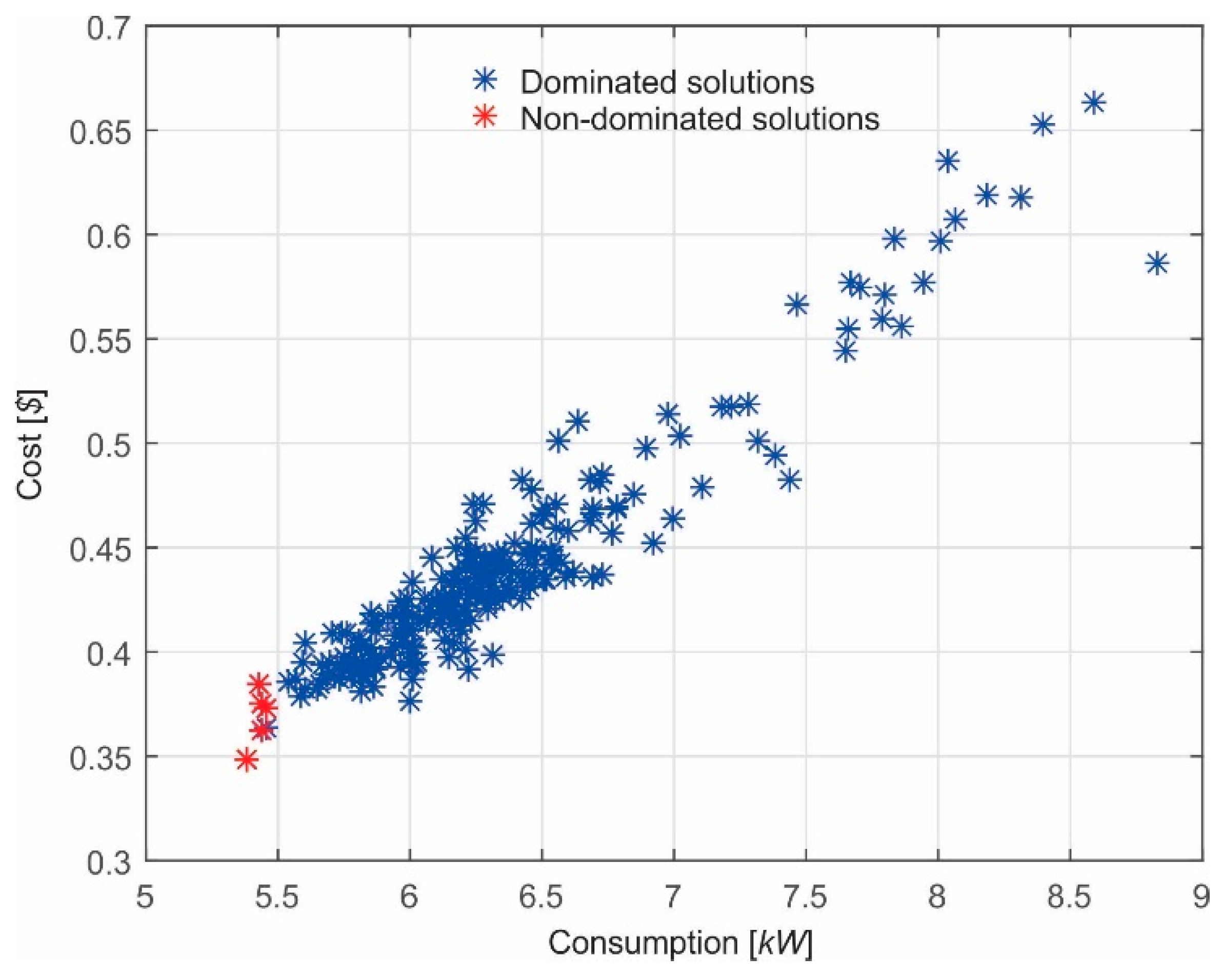
In this work, the extensive solutions search characteristic of the GAs is seized to first obtain an optimal solution in the Pareto and fitness senses at each iteration; then from the resulting set, a new Pareto dominance test is performed and the non-dominated solution with the best fitness is selected. Therefore, the modification of the GA presented in this work shows that it is possible to obtain a simple optimal solution which is optimal in the Pareto sense with the best fitness between the non-dominated set. The modification of the GA proposed is described as follows: as a first step, at each iteration of the GA, individuals of the new population are evaluated to determine whether are optimal in the Pareto sense; when solutions are found that may compose the Pareto set, their fitnesses are evaluated and only the fittest solution is selected, recalling that even though two solutions are optimal in the Pareto sense, they have different fitnesses. In the second step, a similar procedure is performed as in the final part of the first step: the resulting set of “best” solutions is evaluated again to determine optimality in the Pareto sense and the non-dominated solution with the best fitness is selected. With this proposed modification, the obtention of several Pareto set solutions is avoided, improving considerably the performance of the algorithm. A basic outline of both the GA and the Pareto and fitness selection algorithm implemented in this proposal are presented in Algorithm 1 and 2, respectively. It is worth noting that at the end of the first step of Algorithm 1, a set S_φ of solutions is obtained.

Algorithm 1. GA basic outline.
//	First step
1:	P ← InitPopulation
2:	EvalFitness(P)
3:	$S_{\varphi }$← FittestSolution(P)
4:	fork = 1tonum_iterdo
	P′ ← 0
5:	for i = N/2 do
6:	Q ← ParentSelection(P)
7:	if rand[0,1) ≤ $P_{cross}$ then
8:	Q ← Crossover(Q)
9:	end if
10:	if rand[0,1) ≤ $P_{mut}$ then
11:	Q ← Mutation(Q)
12:	end if
13:	P′ ← AddNewSolution(Q)
14:	end for
	SelectSolution(P′)
15:	P ← ReplacePopulation(P′)
	k = k + 1
17:	end for
//	Second step
18:	P′ ← Sφ
19:	SelectSolution(P′)

Algorithm 2. SelectSolution function: Pareto and fitness selection algorithm.
1:	fori = 1toSize(P′)do
2:	for j = 1 to Size(P′) do
3:	if (P′(i).objectives < P′(j).objectives) then
4:	P′(i).NonDominated = true
5:	else
6:	P′(i).NonDominated = false
7:	end if
8:	end for
9:	end for
10:	EvalFitness(P′(i).NonDominated = true)
11:	Sφ ← FittestSolution(P′(i).NonDominated = true)

The crossing operator used in the present work is the so-called “tournament selection” [30], where a group of individuals is randomly selected and then a dispute for the position of father and mother is performed to select the fittest for crossing. P_cross defines the relation between the number of children produced in each generation and the size of the population. A high value of cross probability allows greater and better exploration of the space of solutions. On the other hand, P_mut controls the percentage in which the introduction of new solutions in the population is allowed; if it is very low, many solutions that could have been produced are never tested; if it is very high, there would be a lot of random disturbance, and the children will begin to lose their kinship causing the algorithm lose its ability to learn from the search history. The percentage ranges of P_cross and P_mut recommended by [31] are [75%, 95%] and [5%, 10%], respectively. Finally, it is worth noting that a repairing function is considered in this proposal. The repair functions can be used to bring back to the solution space invalid solutions that are generated due to the randomness of the heuristic problems with restrictions. A simple way to reintroduce an invalid gene into the feasible space of solutions consists of analyzing the genotype in search of bits outside the operational restrictions, applying a force operator to return the bits generated outside these limits within the allowed limits.

Thus, Algorithms 1 and 2 describe the procedure followed by the proposed GA to obtain the optimal solution in the Pareto sense with the best fitness, and are basically used to represent the steps the solutions follow to adjust their chromosomes by crossing and mutation to minimize the objective functions. As each individual is a solution of the optimization problem, the candidate solution is given as input to the objective functions to obtain values representing its fitness. In this evaluation, all input parameters are used by the corresponding objective functions and constraints. Hence, the output of the GA is a simple individual whose chromosome will contain the optimal ON/OFF decisions of all devices for the considered scheduling horizon.

4. Results

In order to numerically evaluate the performance of the proposed HEEMS under different scenarios, three types of tests are performed: the first test considers no solutions of the Pareto front are obtained and the behavior of the HVAC for a day of summer and winter seasons is compared to the results obtained with a freeware tool developed for the energy management of smart residential loads so-called Smart Residential Load Simulator (SRLS) [32]; the second test also considers no solutions of the Pareto set are obtained and the energy consumption and costs are evaluated when renewable energy generation is available in the household. The effect of the energy storage unit is highlighted comparing results to the case when the device is not available; finally, the third test considers a solution of the Pareto front with the best fitness is obtained and results are compared to those obtained when the multi-objective problem is solved considering a commonly used approach such as the weighting approach to define the importance of the different objective functions [7,21]. Practical parameters of the different devices considered in simulations are found in

Table 3. Appliances considered in the present work.

Appliance	Power (kW)
cd	2.5
dw	2.17
es	2.3
ac/ht	1.53/2.4
pp	2
wm	0.2

,

Table 4. HVAC parameters.

αht/ac	βht/ac	ρht/ac	Tmax–Tmin
0.67/0.33	0.044	0.0075	4 °C

,

Table 5. Wind turbine parameters.

Vci (m/s)	Vr (m/s)	Vco (m/s)	Prat (kW)
3.5	12	23	1

,

Table 6. Solar PV panel parameters.

η (%)	A (m2)	Npv	Prat (kW)
15	1.64	13	3.12

and

Table 7. Energy storage unit parameters.

Prc (kW)	Prd (kW)	Pmin/Pmax (kW)		ηc, ηd (%)	δ (%/h)
0.2	0.2	0.8/2	95		0.2

, whereas parameters of the GA are presented in

Table 8. GA parameters.

Parameter	Value
Iterations (num_iter)	100
Population (N)	46
Pcross	95%
Pmut	5%
Selection type	Tournament
Crossing type	Uniform
Mutation type	Complete gene

. To demonstrate how the proposal is able to consider variations in electricity prices as well as variations in the time intervals where prices apply, two different TOU tariffs of two different seasons arbitrarily selected are used in simulations. The optimization model was implemented in the Matlab^® platform installed in an Intel^® i7-7700 desktop computer at 3.60 GHz and 16 Mb of RAM.

4.1. HVAC Behavior Comparison

The first test considers the proposed HEEMS when no solutions of the Pareto front are obtained. Its results are compared to those obtained by the SRLS tool. The objective of the SRLS is to offer a tool capable of simulating the use of different household appliances commonly present in the majority of houses, allowing the end user knowing an estimate of its level of energy consumption and the daily electricity bill to be paid. Simulations are carried out for the HVAC system considering a day of the summer and winter seasons, i.e., tests are performed considering the cooling and heating modes of operation. The TOU tariff considered in simulations is presented in

Table 9. TOU tariff and time intervals for summer.

TOU	Summer		Winter
	Cost ($/kWh)	Interval	Cost ($/kWh)	Interval
off-peak	0.0650	00:00–07:00 19:00–24:00	0.0620	00:00–07:00 19:00–24:00
mid-peak	0.1000	07:00–11:00 17:00–19:00	0.0920	11:00–17:00
on-peak	0.1170	11:00–17:00	0.1080	07:00–11:00 17:00–19:00

(1 May 2012–31 Oct 2012) and winter (1 Nov 2011–30 Apr 2012) seasons.

and obtained from [33]. Results of the SRLS and the HEEMS are presented in Figure 2 and Figure 3, and

Table 10. Energy consumption and costs comparison between the SRLS and the HEEMS for a day of the summer season.

TOU	Energy Consumption (kWh)		Cost ($)		Savings (%)
	SRLS	HEEMS	SRLS	HEEMS
off-peak	3.8380	2.8050	0.2494	0.1823	26.9045
mid-peak	8.9608	2.5500	0.8960	0.2550	71.5401
on-peak	12.9921	0.3825	1.5200	0.0447	97.0592
Total	25.7909	5.7375	2.6654	0.4820	81.9164

and

Table 11. Energy consumption and costs comparison between the SRLS and the HEEMS for a day of the winter season.

TOU	Energy Consumption (kWh)		Cost ($)		Savings (%)
	SRLS	HEEMS	SRLS	HEEMS
off-peak	15.2000	9.6000	0.9424	0.5952	36.8421
mid-peak	3.0000	2.0000	0.2760	0.1840	33.3333
on-peak	4.2000	0.0000	0.4536	0.0000	100.0
Total	22.4000	11.6000	1.6720	0.7792	53.3971

. In these figures, GA_setpoint stands for the setpoint resulting of the HEEMS.

Results presented in Figure 2 and Table 10 show how the HEEMS reduces the activity of the cooling mode of the HVAC, avoiding its operation at intervals where the energy price is higher, i.e., the resulting setpoint of the GA is raised such that the indoor temperature tends to reach the upper limit during intervals of high energy prices. For intervals with lower electricity prices, the device is activated driving the temperature to the lower limit. Opposite to this, the ON/OFF control resulting from the SRLS maintains the temperature within bounds despite electricity prices such that the device is in operation even at intervals of high electricity prices. As a result, the HEEMS achieves savings up to 80%. Similar results are obtained for the winter season. Figure 3 and Table 11 show how the HEEMS avoids the heating operation of the HVAC at intervals of high energy prices. The device is turned ON only when the electricity prices and the outside temperature are low, maintaining the indoor temperature between specified limits. The SRLS drives the HVAC continuously in operation increasing the overall cost. From these results, it is concluded the HEEMS produces appropriate solutions avoiding the end-user discomfort; this is achieved by modifying the HVAC setpoint allowing the indoor temperature to have more variations inside bounds.

4.2. Energy Consumption and Costs Evaluation Considering Renewable Energy Generation and Energy Storage Units

The second test also considers no solutions of the Pareto set are obtained. An evaluation of the energy consumption and costs obtained by the proposed HEEMS is performed when renewable energy generation is available in the household. Two cases are simulated: the first case considers the optimal load scheduling when no energy storage unit is available, and the second case considers the effect of this unit. The TOU tariff considered in simulations is presented in

Table 12. TOU tariff and time intervals for summer.

TOU	Summer		Winter
	Cost ($/kWh)	Interval	Cost ($/kWh)	Interval
off-peak	0.0770	00:00–07:00 19:00–24:00	0.0650	00:00–07:00 19:00–24:00
mid-peak	0.1130	07:00–11:00 17:00–19:00	0.0950	11:00–17:00
on-peak	0.1570	11:00–17:00	0.1320	07:00–11:00 17:00–19:00

(1-May-2017–31-Oct-2017) and winter (1-Nov-2017–30-Apr-2018) seasons.

[33]. Devices operational cycles are defined according to

Table 13. Devices operational cycles.

Device	ti,start-ti,end	di	ti,start-ti,end	di	ti,start-ti,end	di
cd	15:00–24:00	60
dw	12:00–15:00	60	21:00–23:30	60
es	07:00–09:00	30	14:00–16:00	90	20:30–22:30	30
pp	03:00–08:00	60	09:00–15:00	60	19:00–23:00	60
wm	08:00–15:00	90

. Results of simulations are shown in Figure 4 and Figure 5, and

Table 14. Energy consumption and costs for a summer day considering renewable generation and energy storage unit.

TOU	Load Demand (kWh)	Cost ($)	Renewable Generation (kWh)	Resulting Surplus Consumption (kWh)	Renewable Energy Utilization (%)	Optimized Cost ($)	Savings (%)
Off-peak	18.9580	1.4597	18.0870	6.1695	70.7054	0.4750	67.4555
Mid-peak	8.9272	1.0088	14.7150	3.3061	38.1997	0.3735	62.9758
On-peak	11.8180	1.8554	21.0490	0	56.1451	0	100
Total	39.7030	4.3239	53.8510	9.4756	56.1315	0.8486	80.3741

and

Table 15. Energy consumption and costs for a winter day considering renewable generation and energy storage unit.

TOU	Load Demand (kWh)	Cost ($)	Renewable Generation (kWh)	Resulting Surplus Consumption (kWh)	Renewable Energy Utilization (%)	Optimized cost ($)	Savings (%)
Off-peak	18.4710	1.2006	18.1280	6.9981	63.2882	0.4548	62.1189
Mid-peak	12.3230	1.1706	22.4290	0.0321	54.7991	0.0030	99.7437
On-peak	10.1460	1.3392	11.7900	0.7299	79.8651	0.0963	92.8091
Total	40.9500	3.7104	52.3470	7.7601	63.4036	0.5541	85.0663

.

The dashed red line shown in Figure 4 corresponds to the load profile obtained by the HEEMS when no energy storage unit is available. It is observed that the load dispatch avoids on-peak time intervals, however, there are intervals where energy must be drawn from the power system not taking advantage of the renewable energy available. The black line of Figure 4 corresponds to the case when an energy storage unit is considered. It can be noticed how the energy drawn from the power system has been reduced. The effect of the storage unit is evident since stores energy at times when the energy has low prices and when there is renewable energy availability and delivers energy when there is load surplus. Both cases show how the total renewable energy is not fully used. However, the numerical results presented in Table 14 show a significant reduction in the energy costs up to 80% and renewable energy utilization up to 50%. It is worth noting that there is a small amount of energy consumption on the on-peak time interval, this is due to the fact the es device is set by the user to operate between 14:00–16:00 h with an operating cycle of 90 min, such that the HEEMS has no option but schedule the device despite the high electricity price.

A similar behavior for the winter day is shown in Figure 5. The change in the TOU intervals is properly considered by the HEEMS. However, as in the previous case, it can be noticed how there is load dispatched at intervals of high energy cost. Again, this is owing to the fact that the es operational window is defined by the user overlapping the first interval of high prices, such that the HEEMS has no choice but dispatching this load. In the second high-price interval the cd is dispatched, this may be no optimal from the operational point of view, but the HEEMS has adjusted all its variables to reduce the overall cost. As explained in the next subsection, better solutions are achieved when solutions of the Pareto front are obtained. Results presented in Table 15 highlight the availability of the energy storage unit since saving up to 85% are obtained. This is a consequence of the better renewable energy utilization reaching values of 63%.

4.3. Energy Consumption and Costs Evaluation Considering Solutions of the Pareto Front

The third test evaluates the energy consumption and costs considering the calculation of solutions of the Pareto front as explained in Section 3. To highlight the HEEMS performance, the Pareto front solution with the best fitness is compared to the solution when the multi-objective optimization problem is solved assigning weights to each objective function as proposed in [24]. The resulting objective function may be written as:

$$F={\omega }_1{f}_1+{\omega }_2{f}_2,$$

where weights are calculated by running the model with the individual objective functions, i.e., using f₁ and f₂ as an individual objective function, which results in objective function values of X kWh, and $Y, respectively. Thus, the weights can be defined as follows:

$${\omega }_1=Y/X,{\omega }_2=1,$$

Solutions of the Pareto front are shown in Figure 6. It is observed that the red points correspond to solutions of the Pareto front, i.e., are the non-dominated set resulting from the first step of Algorithm 1. Between these solutions, the solution with the best fitness is selected and corresponds to values of energy consumption of 5.3861 kWh with a cost of $0.3484. From the comparison results presented in

Table 16. Comparison between the HEEMS solution and a multi-objective solution based on weights.

Multi-Objective (Weights)				HEEMS
Tariff	RenewableEnergy Utilization (%)	Resulting Surplus Consumption (kWh)	Cost ($)	RenewableEnergy Utilization (%)	Resulting Surplus Consumption (kWh)	Cost ($)	Savings (%)
Off-peak	54.74	5.2867	0.3436	57.07	5.0070	0.3104	9.6623
Mid-peak	38.44	0.9886	0.0939	48.64	0.1861	0.0171	81.7891
On-peak	51.07	0.2393	0.0315	51.31	0.1929	0.0208	33.9682
Total	52.21	6.5145	0.4691	55.10	5.3861	0.3484	25.7301

, it is shown how the selected solution improves the outcomes of the HEEMS, achieving savings up to 25% when compared to the solutions when weights are used to solve the multi-objective problem. Furthermore, it is shown in Figure 7 how the HEEMS better utilizes the energy availability scheduling the majority of loads inside the shaded area representing renewable energy generation. Finally, it is important to mention that the time the HEEMS took to obtain the solution was 16.3 s, a very short computational time compared to previously proposed approaches, which confirms the applicability of the proposal.

4.4. Scope and Limitations of the Proposal

The scope of the proposed HEEMS is tho develop an algorithm for the optimal scheduling of residential loads taking into account factors such as electricity proces, ambient temperature, end-user preferences, and the influence of the human activity on the temperature inside a house. The main goal is to reduce computational times and human interaction such that the algorithm.

5. Conclusions

A heuristic algorithm for a HEEMS has been proposed in this paper. The proposed optimization model minimizes the energy consumption and costs subject to household devices’ operational constraints considering the renewable energy availability. For that purpose, the on-site energy generation and storage were considered adapting models of the wind turbine, solar PV panels, and energy storage unit. The impact of the human activity inside a house on the energy consumption was also considered including a previously proposed AL index to the model of the HVAC device; this index was calculated using an open-source data set of electricity consumption and occupancy. The resulting multi-objective optimization problem was solved with a proposed modified GA. The modified GA calculates solutions of the Pareto front with the best fitness at each iteration in order to obtain a reduced set of solutions; at the end of the GA iterations, a new Pareto dominance test is performed to the reduced set of solutions and the solution with the best fitness is selected, this reduces the human interaction as compared to previously proposed approaches, representing a contribution of the present work. From the results presented, it was shown how the HEEMS is able to optimally schedule the household devices considering the TOU electricity tariff with very low computational times. For the case of the HVAC device, it was presented in details how the HEEMS optimally manages the device´s setpoint to drive the indoor temperature between bounds reducing the energy consumption and costs while maintaining the end-user comfort. Finally, it was shown how the HEEMS improves the results obtained as compared to the approach of weighting when solving the multi-objective optimization problem.

References

1. The Smart Grid: An Introduction; US Department of Energy: Washington, DC, USA, 2017. Available online: https://www.energy.gov/sites/prod/files/oeprod/DocumentsandMedia/DOE_SG_Book_Single_Pages%281%29.pdf (accessed on 5 February 2019).
2. Energy Independence and Security Act of 2007 (EISA 2007). Available online: https://www.congress.gov/bill/110th-congress/house-bill/6 (accessed on 5 February 2019).
3. Mosaddegh, A.; Cañizares, C.A.; Bhattacharya, K. Optimal demand response for distribution feeders with existing smart loads. IEEE Trans. Smart Grid 2017, 9, 5291–5300. [Google Scholar] [CrossRef]
4. O’Connell, N.; Pinson, P.; Madsen, H.; O’Malley, M. Benefits and challenges of electrical demand response: A critical review. Renew. Sustain. Energy Rev. 2014, 39, 686–699. [Google Scholar] [CrossRef]
5. Beaudin, M.; Zareipour, H. Home energy management systems: A review of modelling and complexity. Renew. Sustain. Energy Rev. 2015, 45, 318–335. [Google Scholar] [CrossRef]
6. Zhou, B.; Li, W.; Chan, K.W.; Cao, Y.; Kuang, Y.; Liu, X.; Wang, X. Smart home energy management systems: Concept, configurations, and scheduling strategies. Renew. Sustain. Energy Rev. 2016, 61, 30–40. [Google Scholar] [CrossRef]
7. Paterakis, N.G.; Medeiros, M.F.; Catalo, J.P.S.; Siaraka, A.; Bakirtzis, A.G.; Erdinc, O. Optimal daily operation of a smart-household under dynamic pricing considering thermostatically and non-thermostatically controllable appliances. In Proceedings of the IEEE 5th International Conference on Power Engineering, Energy and Electrical Drives, Riga, Latvia, 11–13 May 2015. [Google Scholar] [CrossRef]
8. Zheng, M.; Meinrenken, C.J.; Lackner, K.S. Smart households: Dispatch strategies and economic analysis of distributed energy storage for residential peak shaving. Appl. Energy 2015, 147, 246–257. [Google Scholar] [CrossRef] [Green Version]
9. Geem, Z.W.; Kim, J.H.; Loganathan, G. A new heuristic optimization algorithm: Harmony search. Simulation 2001, 76, 60–68. [Google Scholar] [CrossRef]
10. Ozkan, H.A. A new real time home power management system. Energy Build. 2015, 97, 56–64. [Google Scholar] [CrossRef]
11. Ahmed, M.S.; Mohamed, A.; Khatib, T.; Shareef, H.; Homod, R.Z.; Ali, J.A. Real time optimal schedule controller for home energy management system using new binary backtracking search algorithm. Energy Build. 2017, 138, 215–227. [Google Scholar] [CrossRef]
12. Salinas, S.; Li, M.; Li, P. Multi-objective optimal energy consumption scheduling in smart grids. IEEE Trans. Smart Grid 2013, 4, 341–348. [Google Scholar] [CrossRef]
13. Soares, A.; Gomes, A.; Antunes, C.H.; Oliveira, C. A customized evolutionary algorithm for multiobjective management of residential energy resources. IEEE Trans. Ind. Inform. 2017, 13, 492–501. [Google Scholar] [CrossRef]
14. Lacerda, H.F.; Feitosa, A.R.S.; Silva-Filho, A.G.; Santos, W.P.; Cordeiro, F.R. SmartHome energy saving using a multi-objective approach based on appliances usage profiles. In Advances in Artificial Intelligence; Springer International Publishing: Cham, Switzerland, 2017; pp. 142–147. ISBN 978-3-319-57351-9. [Google Scholar]
15. Veras, J.M.; Silva, I.R.S.; Pinheiro, P.R.; Rabelo, R.A.L.; Veloso, A.F.S.; Borges, F.A.S.; Rodrigues, J.J.P.C. A multi-objective demand response optimization model for scheduling loads in a home energy management system. Sensors 2018, 18, 3207. [Google Scholar] [CrossRef] [PubMed]
16. Bilil, H.; Aniba, G.; Gharavi, H. Dynamic appliances scheduling in collaborative microgrids system. IEEE Trans. Power Syst. 2017, 32, 2276–2287. [Google Scholar] [CrossRef] [PubMed]
17. Khalid, R.; Javaid, N.; Rahim, M.H.; Aslam, S.; Sher, A. Fuzzy energy management controller and scheduler for smart homes. Sustain. Comput. Inform. Syst. 2019, 21, 103–118. [Google Scholar] [CrossRef]
18. Khemakhem, S.; Rekik, M.; Krichen, L. Double layer home energy supervision strategies based on demand response and plug-in electric vehicle control for flattening power load curves in a smart grid. Energy 2019, 167, 312–324. [Google Scholar] [CrossRef]
19. Ranjith, R.; Prakash, N.K.; Vadana, D.P.; Pillai, A.S. Smart Home Energy Management System—A Multicore Approach. In International Conference on Advanced Computing Networking and Informatics; Kamal, R., Henshaw, M., Nair, P., Eds.; Springer: Singapore, 2019; Volume 870, pp. 363–370. ISBN 978-981-13-2672-1. [Google Scholar]
20. Daneshvar, M.; Pesaran, M.; Mohammadi-ivatloo, B. Transactive energy in future smart homes. In The Energy Internet; Su, W., Huang, A.Q., Eds.; Woodhead Publishing: Cambridge, UK, 2019; pp. 153–179. ISBN 978-0-08-102207-8. [Google Scholar]
21. Bozchalui, M.C.; Hashmi, S.A.; Hassen, H.; Canizares, C.A.; Bhattacharya, K. Optimal operation of residential energy hubs in smart grids. IEEE Trans. Smart Grid 2012, 3, 1755–1766. [Google Scholar] [CrossRef]
22. Bhuiyan, F.A.; Yazdani, A.; Primak, S.L. Optimal sizing approach for islanded microgrids. IET Renew. Power Gener. 2015, 9, 166–175. [Google Scholar] [CrossRef]
23. Hassen, H. Implementation of Energy Hub Management System for Residential Sector. Master’s Thesis, Electrical and Computer Engineering, University of Waterloo, Waterloo, ON, Canada, 2010. [Google Scholar]
24. Bozchalui, M.C. Optimal Operation of Energy Hubs in the Context of Smart Grids. Ph.D. Thesis, Electrical and Computer Engineering, University of Waterloo, Waterloo, ON, Canada, 2011. [Google Scholar]
25. Giorsetto, P.; Utsurogi, K.F. Development of a new procedure for reliability modeling of wind turbine generators. IEEE Trans. Power Appar. Syst. 1983, PAS-102, 134–143. [Google Scholar] [CrossRef]
26. Lee, D.; Wang, L. Small-signal stability analysis of an autonomous hybrid renewable energy power generation/energy storage system part I: Time-domain simulations. IEEE Trans. Energy Convers. 2008, 23, 311–320. [Google Scholar] [CrossRef]
27. Eco data set (Electricity Consumption and Occupancy). Available online: http://rossa-prod-ap11.ethz.ch/delivery/DeliveryManagerServlet?dps_pid=IE594964 (accessed on 4 December 2018).
28. Past Weather in Zürich. Available online: https://www.timeanddate.com/weather/switzerland/zurich/historic?month=6&year=2012 (accessed on 7 January 2019).
29. Goldberg, D.E. Genetic Algorithms in Search, Optimization and Machine Learning; Addison-Wesley Longman Publishing Co.: Boston, MA, USA, 1989; ISBN 0201157675. [Google Scholar]
30. Miller, B.L.; Goldberg, D.E. Genetic algorithms, tournament selection, and the effects of noise. Complex Syst. 1995, 9, 193–212. [Google Scholar]
31. Srinivas, M.; Patnaik, L.M. Genetic algorithms: A survey. Computer 1994, 27, 17–26. [Google Scholar] [CrossRef]
32. Gonzalez-Lopez, J.M.; Pouresmaeli, E.; Cañizares, C.A.; Bhattacharya, K.; Mosaddegh, A.; Solanki, B.V. Smart residential load simulator for energy management in smart grids. IEEE Trans. Ind. Electron. 2019, 66, 1443–1452. [Google Scholar] [CrossRef]
33. Ontario Hydro. Available online: http://www.ontario-hydro.com/historical-rpp-rates (accessed on 7 January 2019).
Figure 1. Activity level (AL) of a Swiss house for the hottest day of summer 2012.
Energies 12 00671 g001
Figure 2. HVAC behavior comparison between a solution of the SRLS and a solution of the HEEMS for a day of the summer season: (a) SRLS solution; (b) HEEMS solution.
Energies 12 00671 g002
Figure 3. HVAC behavior comparison between the solution of the SRLS and a solution of the HEEMS for a day of the winter season: (a) SRLS solution; (b) HEEMS solution.
Energies 12 00671 g003
Figure 4. Resulting power consumption profile for a summer day with and without energy storage unit.
Energies 12 00671 g004
Figure 5. Resulting power consumption profile for a winter day with and without energy storage unit.
Energies 12 00671 g005
Figure 6. Dominated and non-dominated solutions of the Pareto front.
Energies 12 00671 g006
Figure 7. Results of power consumption profile for a summer day: (a) minimization based on weights; (b) HEEMS solution.
Energies 12 00671 g007aEnergies 12 00671 g007b