Article

Pollution Events at the High-Altitude Mountain Site Zugspitze-Schneefernerhaus (2670 m a.s.l.), Germany

1
Professorship of Ecoclimatology, Technische Universität München, 85354 Freising, Germany
2
Climate Research Division, Environment and Climate Change Canada, Toronto, ON M3H 5T4, Canada
3
Professorship of Environmental Sensing and Modeling, Technische Universität München, 80333 Munich, Germany
4
Institute for Advanced Study, Technische Universität München, 85748 Garching, Germany
5
German Environment Agency (UBA), 82475 Zugspitze, Germany
6
Physical Geography and Climatology, RWTH Aachen University, 52056 Aachen, Germany
7
Department for Safety and Radiation Protection, Technische Universität München, 85748 Garching, Germany
8
Heidelberg Center for the Environment, Universität Heidelberg, 69120 Heidelberg, Germany
*
Author to whom correspondence should be addressed.
Atmosphere 2019, 10(6), 330; https://doi.org/10.3390/atmos10060330
Submission received: 7 May 2019 / Revised: 12 June 2019 / Accepted: 14 June 2019 / Published: 18 June 2019

Abstract

:
Within the CO2 time series measured at the Environmental Research Station Schneefernerhaus (UFS), Germany, as part of the Global Atmospheric Watch (GAW) program, pollution episodes are traced back to local and regional emissions, identified by δ13C(CO2) as well as ratios of CO and CH4 to CO2 mixing ratios. Seven episodes of sudden enhancements in the tropospheric CO2 mixing ratio are identified in the measurements of mixing/isotopic ratios during five winter months from October 2012 to February 2013. The short-term CO2 variations are closely correlated with changes in CO and CH4 mixing ratios, achieving mean values of 6.0 ± 0.2 ppb/ppm for CO/CO2 and 6.0 ± 0.1 ppb/ppm for CH4/CO2. The estimated isotopic signature of CO2 sources (δs) ranges between −35‰ and −24‰, with higher values indicating contributions from coal combustion or wood burning, and lower values being the result of natural gas or gasoline. Moving Keeling plots with site-specific data selection criteria are applied to detect these pollution events. Furthermore, the HYSPLIT trajectory model is utilized to identify the trajectories during periods with CO2 peak events. Short trajectories are found covering Western and Central Europe, while clean air masses flow from the Atlantic Ocean and the Arctic Ocean.

1. Introduction

Since the beginning of the industrial era, atmospheric greenhouse gas (GHG) concentrations have been rapidly increasing due to fossil fuel burning and deforestation [1]. Carbon dioxide (CO2) is the most important anthropogenic GHG, and its concentration has increased by more than 45% from the pre-industrial level of 278 ppm (parts per million) to 405 ppm in the year 2017 [2]. Continuous atmospheric CO2 measurements significantly contribute to a better understanding of the global carbon cycle and its effect on the earth’s climate. The Environmental Research Station Schneefernerhaus (UFS) has been part of the Global Atmospheric Watch (GAW) program of the World Meteorological Organization (WMO). Due to its remote and elevated location, the UFS is relatively less influenced by direct anthropogenic emissions and thus measurements of background concentrations there can be regarded as representative of a larger region [3,4]. Nevertheless, the station is occasionally influenced by local-to-regional emissions due to the air mass transport of polluted boundary layer air and/or local effects. These polluted air masses contain signals from continental sources, as indicated by the high variability in trace gas concentrations on time scales of hours and days [5]. In order to improve the retrieval of atmospheric background CO2 concentrations from measurements at these remote sites, it is crucial to investigate these pollution-affected periods systematically, as well as to identify their source regions.
In order to study sudden increases and short-term variability in atmospheric trace gases at mountain stations, in situ measurements of trace gases with anthropogenic sources as well as statistical trajectory methods have been frequently applied to define the source, identify its origin, and elucidate and characterize the causes of the variation. For instance, Apadula et al. [6] analyzed atmospheric CO2 concentrations at three Alpine sites (Plateau Rosa and Monte Cimone in Italy, and Zugspitze in Germany) and identified a short-lived episode of large fluctuations in the CO2 mixing ratios. This was similarly observed at Plateau Rosa and Zugspitze, but with a delay of 12–18 h, as shown by backward trajectory and cluster analysis. Kaiser et al. [7] detected the potential source of nitrogen oxides (NOx), carbon monoxide (CO), and ozone (O3) using trajectory residence time statistics at five Alpine GAW stations (Zugspitze/Hohenpeissenberg (Germany), Sonnblick (Austria), Jungfraujoch (Switzerland), and Mt. Krvavec (Slovenia)). Furthermore, Uglietti et al. [8] investigated the transport of air masses with high CO2 levels to the Jungfraujoch station (JFJ) using backward Lagrangian particle dispersion model simulations, and employed CO2 and oxygen (O2) signatures to classify these air masses. Tuzson et al. [9] focused on the pronounced enhancement in the tropospheric CO2 at Jungfraujoch in February 2009. During this period, four events were captured in which CO and CO2 mixing ratios were highly correlated as a proxy for fossil fuel CO2, as well as the CO2 mixing ratio and isotopic composition of atmospheric CO2 δ13C, using the Keeling method. Ferrarese et al. [10] identified two significantly high CO2 concentration events at four high-altitude European stations in February 2004 using the backward trajectories of the polluted air masses from the European boundary layer as indicated by CO and O3. Ghasemifard et al. [4] showed that the high CO2 mixing ratios in winter (from the year 2012 to 2014) at the UFS originated in the German Ruhr area, the Netherlands, and Lusatia (an area bounded by Germany, Poland, and the Czech Republic) based on CO2 and δ13C measurements, as well as potential source contribution functions (PSCFs).
δ13C has been used in numerous studies to gain insight into different aspects of the carbon cycle (e.g., [9,11]). Nevertheless, the isotopic composition of atmospheric CO2 is related to the atmosphere–biosphere exchange, because the terrestrial ecosystem (photosynthesis/respiration) and air–sea gas exchanges differently discriminate against 13C [12,13]. Therefore, the δ13C signature is often used to distinguish CO2 contributions from oceanic, biospheric, and anthropogenic CO2 emissions [14]. Furthermore, since different CO2 emitters have different δ13C signatures, the carbon isotope ratio enables the identification and quantification of CO2 emitters and their underlying mechanisms at the local to regional levels [15]. Various ranges of δ13C have been obtained for combustion sources: −44‰ to −37‰ for natural gas combustion, −32‰ to −26‰ for gasoline combustion, −27‰ to −24‰ for coal combustion, and −27‰ to −22‰ for wood combustion [14,16,17,18].
It is well known that a large amount of global CO, which is produced by the incomplete oxidation of carbon, originates from anthropogenic sources. Moreover, approximately 70% of the total sources of CO in Europe are anthropogenic [19]. Thus, with CO as a tracer, anthropogenic CO2 emissions from fossil fuel combustion, and therefore CO2 emissions from regional sources, can be identified (e.g., [9,20,21,22]). The ratio of atmospheric CO to CO2 (CO/CO2) has been utilized to quantify fossil fuel contribution in relation to CO2 variations, and to determine the type of combustion and burning efficiency; high ratios indicate poor burning and trace traffic emissions [9,23,24].
Methane (CH4), the second most essential anthropogenic GHG gas after CO2, has increased from the pre-industrial level of 722 ppb to the present level of 1859 ppb (2017) due to increased emissions from anthropogenic sources [2]. CH4 is emitted from a variety of natural and anthropogenic sources and also from ground level sources (e.g., ruminants, natural gas leakages, coal mining, or waste deposits). The source of CH4 in Western Europe is mainly anthropogenic [25]. Though vehicle emissions are an insignificant source on a global scale [26], they can count for up to 30% of total emissions in areas with high traffic density [27]. Several studies have shown that there exist positive correlations between atmospheric CO2 and CH4 mixing ratios mostly in the winter (e.g., [28,29]). Based on the assumption that CO2 and CH4 originate from similar sources and sinks, the CH4 to CO2 emission ratio (CH4/CO2) is utilized to filter observed atmospheric CO2 data influenced by local sources/sinks [30].
In this study, we performed the analysis from 1 October 2012 to 1 March 2013 at the UFS/Zugspitze. During this period, we captured several consecutive short-term pollution events with a strong increase (>~15 ppm) in the measured CO2 concentration. The period was restricted to these five months of autumn/winter in order to minimize the effect of biological activities (such as photosynthesis and respiration) in the interpretation of pollution signals. It was found that employing the in situ measurements of isotopic signatures of CO2 using δ13C(CO2), the emission ratios of CO/CO2 and CH4/CO2, and the backward trajectories from the HYSPLIT (Hybrid single-particle Lagrangian integrated trajectory model) provided essential information for the identification, characterization, and source estimation of pollution events, as shown in the subsequent sections.

2. Material and Methods

2.1. Measurement Site

The high Alpine Environmental Research Station Schneefernerhaus (UFS) is located in the northern Alps at an altitude of 2650 m above see level (a.s.l.) (47° 25′ N, 10° 59′ E), nearly 300 m below the summit of Mount Zugspitze, the highest mountain in Germany, and about 90 km southwest of Munich. The UFS is often above the planetary boundary layer (PBL) and receives well-mixed and/or free tropospheric air masses [31]. Nevertheless, UFS is occasionally influenced by regional emissions such as the transport of PBL air masses due to thermally induced flow systems [5,32,33,34], although this issue can be addressed by characterizing the measurements based on their air mass histories and origins. Further detailed site information is given in the GAW station information system [35].

2.2. Analyzers and Sampling Systems

In this study, all instruments were operated at the German Environment Agency (Umweltbundesamt, UBA) laboratory and connected to the same air inlet (2670 m a.s.l.); thus, they measured the same air samples.
We measured CO2 and δ13C(CO2) with a Picarro G1101-i analyzer (manufactured in 2010 by Picarro Inc., USA, and measuring at a rate of 0.1 Hz) and calibrated them using two standard gases with high and low concentrations (standard 1:350.1 ± 0.5 ppm CO2 mixing ratio and −3.3‰ ± 0.2‰ δ13C; standard 2:503.4 ± 0.5 ppm CO2 mixing ratio and −20.0‰ ± 1.0‰ δ13C) in synthetic air. Details on our air sampling inlet and calibration systems are presented in Ghasemifard et al. [4]. Notably, this analyzer was not upgraded to account for the spectral interferences caused by methane (bias δ13C by 0.4‰ CH4 ppm−1) and water vapor (including water vapor dilution, water vapor pressure broadening, and HDO spectral interference effects). Several studies have evaluated and validated the G1101-i analyzer measurements before and after upgrading in comparison with other measurement devices [4,36,37,38,39,40]. As described by Ghasemifard et al. [4], the measured CO2 and δ13C were post-corrected, in which parallel measured CO2, H2O, and CH4 were employed.
The UBA performed CH4 measurements with a Picarro EnviroSense 3000i analyzer (using cavity ring-down spectroscopy) and recorded CO data by an Aero-Laser AL5002 (ultraviolet-fluorescence instrument). Further, the UBA carried out calibration and quality assurance for these atmospheric compounds following GAW quality standards. The UBA station standards for interconnection with the international standard reference were reported on the WMO/NOAA-2004 scale for CO and WMO X2004a scale for CH4 by National Oceanic and Atmospheric Administration (NOAA), Boulder, Colorado.
For this study, we aggregated the data of CO, CH4, CO2, and δ13C to hourly averages by the statistical program R [41] and employed the R packages Openair [42] and ggplot2 [43] for further analyses.

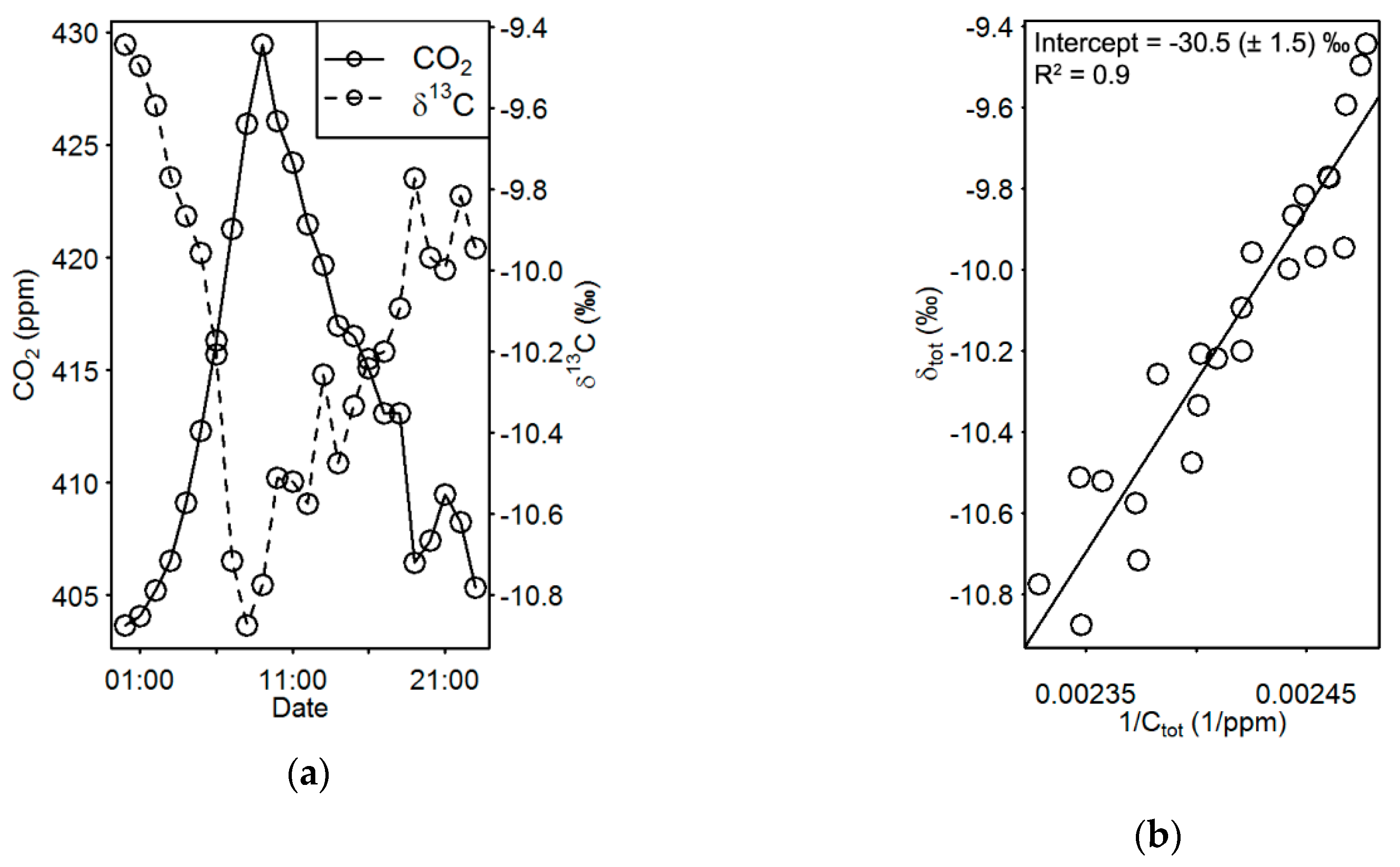
2.3. Keeling Plot Method

In order to calculate the mean isotopic signature of a source, the Keeling plot method [44,45] links variations in CO2 and δ13C by adding CO2 from that source to the background atmospheric CO2 mixing ratio and background isotopic ratio [46]. The mass balance of the total CO2 is
C t o t = C b g + C s
where Ctot, Cbg, and Cs respectively refer to the total measured CO2 mixing ratio, background CO2 mixing ratio, and source CO2 mixing ratio. Given the mass balance,
δ t o t · C t o t = δ b g · C b g + δ s · C s
where δ represents δ13C of each CO2 component. Rearranging and combining Equations (1) and (2) yields
δ t o t = C b g / C t o t ( δ b g δ s ) + δ s
In the case of a single-source pollution event, a plot of the measured (total) δ13C versus 1/CO2 yields a straight line with a y-intercept of δ s . It is crucial to observe that Equation (3) of the Keeling method involves two basic prerequisites. Firstly, the background and isotopic signature of the source need to be constant. Secondly, sources and sinks of different isotopic signatures may not co-occur during the observation [15]. The effect of disregarding these criteria is also graphically depicted in Vardag et al. [46]. Note that the background value does not have to be known in order to calculate the mean source signature [15].
As an example, Figure 1a shows one of the events in this study (E7), while Figure 1b displays the corresponding Keeling plot.
In order to calculate the source signature as an intercept, a linear regression needs to be fitted to the data (e.g., Figure 1b). Miller and Tans [47] compared two models for the regression, Model I (ordinary least-squares regression in which only y-errors are taken into account), and Model II (regression fit; e.g., weighted total least squares (WTLS), which accounts for errors on both x and y [48]). Miller and Tans [47] found that Model I is biased for the intercept, even when the values of R2 are high. Therefore, in this paper, we employed WTLS to fit the linear regression in the Keeling method.
Based on the classical Keeling plot method, Vardag et al. [46] presented a method to accurately determine the source signature for a continuous data set (moving Keeling plot approach) following Equation (3). The advantage of this approach is that the prerequisites of the Keeling approach do not have to be checked individually for the entire data set, which would be very tedious for a continuous long-term data set. This method provides correct results only when a number of criteria are fulfilled. These criteria then automatically discard situations in which sources and sinks occur simultaneously and in which the mean source signature or the background value change. Note that the optimal set of parameters was found by Vardag et al. [46] and validated using a simulated data set in Heidelberg. The individual filter criteria and the rationale behind the filter criteria are adopted from Vardag et al. [46] and listed in Table 1.
Moreover, there is another criterion in Vardag et al. [46] that is not applicable in this study, namely an increase in the CO2 mixing ratio by more than 5 ppm. Simultaneously occurring sources and sinks bias the retrieved source signature more strongly the smaller the net CO2 signal is. Therefore, the criterion is chosen to exclude periods where the photosynthetic sink is similarly strong to the total CO2 sources. Vardag et al. [46] report that a threshold of 5 ppm is sufficient to eliminate strongly biased source signatures in Heidelberg, a medium-sized city that is strongly influenced by local sinks and sources and located about 20 km southwest of an industrial area (Mannheim/Ludwigshafen) [22]. In contrast, the UFS is a remote mountain site where there is no sudden or direct influence from the photosynthetic sink [4]. Therefore, provided that there is an increase in CO2, the second criterion (>5 ppm) is redundant. Regarding the applied criteria in Table 1, note that we also tested shorter periods (i.e., 4 and 3 h/data point); however, the number of events detected was the same. Therefore, the initial 5 h period was preferred since a higher number of data points will supposedly yield more reliable results.
Seven events within the study period satisfied the criteria for the moving Keeling approach (see Table 2).
In Section 3.1, the moving Keeling approach is presented in parallel to the classical Keeling plot in order to detect the pollution source signature at the UFS. The moving Keeling plot method works so that, for example, for the determination of the mean source signature at 14:00 h, we use the hourly CO2 and δ13C measurements from 12:00 h to 16:00 h and fit a regression line. To select episodes for the classical Keeling plots, periods with a CO2 increase of more than ~15 ppm within timescales of hours and days were selected (see Table 2). In order to provide comparability with the moving Keeling plot analysis we removed the non-monotonously increasing parts of those episodes and considered only the front shoulder of the CO2 mixing ratios. If we considered the latter selection in the example of Figure 1, the source signature would be −33.8 ± 1.7‰ instead of −30.5 ± 1.5‰, due to the bias caused by the decreasing part of the event.

2.4. Emission Ratio

In order to determine the emission ratios (slope of the regression) and accuracy (coefficient of determination R2), we examined the relationship between the CO and CO2, as well as the CH4 and CO2 mixing ratios using scatter plots and fitted linear regressions, respectively. However, there are different approaches to determining the emission ratios (CO/CO2 and CH4/CO2). Occasionally the emission ratios are calculated as ΔCO/ΔCO2 or ΔCH4/ΔCO2, where Δ denotes the difference of the total concentration to the background concentration (which is individually defined using particular techniques (e.g., [49,50])). In some studies, the emission ratio is calculated as CO/ΔCO2, whereas sometimes no background is removed (e.g., [51,52]). In this paper, in order to be consistent with the Keeling plot data selection, we calculated emission ratios on the total emission ratios for periods from the minimum (when the CO2 mixing ratio started to increase) to the maximum (when the highest value of the CO2 mixing ratio was reached). Table 2 presents the corresponding lengths of these periods for each event.

2.5. HYSPLIT Trajectory Model

We employed the HYSPLIT (hybrid single-particle Lagrangian integrated trajectory) model in order to study air transport during the episodes and characterize the CO2 source regions [53,54]. The underlying meteorological model was obtained from the Global Forecast System and driven by 3-h forecast weather data at a 0.5° resolution. We calculated hourly backward trajectories for the 96 h before the air masses reached the UFS. The terrain altitude for the trajectory starting point at the UFS is 1312.4 m a.s.l. in the model. Thus, back trajectory calculation was started at an altitude of 1500 m above ground level (a.g.l.), resulting in 2812 m a.s.l., which roughly matches the sample inlet height (2670 m a.s.l.).

2.6. PSCF

Additionally, we utilized the potential source contribution function (PSCF) method [55,56] to plot the spatial distribution of potential geographic source locations. The PSCF calculates the probability (0 ≤ P i j ≤ 1) that a potential source is located at latitude i and longitude j . Therefore, an air parcel passing through that location along the trajectory to the receptor site collects the material and characteristics from the source. The probability for a given cell is defined as P i j =   m i j / n i j , where n i j is the total number of times that the trajectories pass through the cell ( i , j ) and m i j is the number of trajectories associated with concentration values at the receptor site greater than a specific threshold. In this study, the threshold was set to be the 90th percentile of the CO2 mixing ratio and the 24 h measurement before and after each event is included in the 90th percentile calculation.

3. Results and Discussion

Figure 2 shows a high-resolution time series of the CO2 mixing ratio, corresponding the δ13C values, CO mixing ratio, and CH4 mixing ratio from October 2012 to February 2013. According to Figure 2, episodes of high CO2 concentrations are observed during similar periods of CO and CH4 mixing ratios. These episodes are labeled E1–E7. The mixing ratios of all three trace gases are highly correlated, while δ13C was anti-correlated to the CO2 mixing ratio. In subsequent sections, we present a detailed investigation of the seven episodes exhibiting high CO2. Table 2 contains the date, duration of each episode, and duration of their increasing part (i.e., from the start of the increase to the moment the maximum CO2 concentration is reached).

3.1. δ13C(CO2) and Keeling Plot

Figure 3a shows the resulting isotope signatures for each event using the classical Keeling plot method. It has to be noted again that only the increasing parts of each event are considered for this calculation. The intercept values range between −35‰ and −24‰, and δ13Cs is most enriched in E1 (−24.2‰ ± 1.2‰) and most depleted in E4 (−34.9‰ ± 0.6‰). For all the events, the δ13C to the 1/CO2 relationship is well described by the WTLS regression with a high coefficient of determination (>0.90); except for one case (E5, R2 = 0.82). The error bars in Figure 3a are the intercept error, which is listed in Table S1 and calculated by WTLS regression.
The averaged δ13Cs signatures (Figure 3a) (i.e., −29‰) are in agreement with the signatures (−20‰ to −30‰) determined by Tuzson et al. [9] at the high Alpine research station Jungfraujoch (JFJ) at an altitude of 3580 m a.s.l. This 13C signature represents a typical isotopic combination of anthropogenic and biological sources. The higher values of E1 and E2 (−24.2‰ ± 1.2‰ and −26.3‰ ± 0.9‰) suggest a significant contribution from coal combustion or wood burning, while the low values of E3–E7 (−34.9‰ to −29.6‰) are consistent with contributions from natural gas or gasoline [14,16].
The moving Keeling plot method with the specified data selection criteria (see Section 2.4) was employed to detect pollution events at the UFS automatically. The moving Keeling plot calculated the source signature for each of the five data points (i.e., 5 h), and depending on the length of the event, it generated several values per event; thus, the detected isotopic source signatures are presented as box plots. The whiskers of the boxplots indicate the minimum and maximum values, the lower and upper boundaries of the boxes are 25th- and 75th-percentiles, and the horizontal lines inside the boxes represent medians. The mean difference between the mean value of the classical and moving Keeling plots is 0.0‰ ± 0.5‰. This result confirms the reliability of the applied criteria.

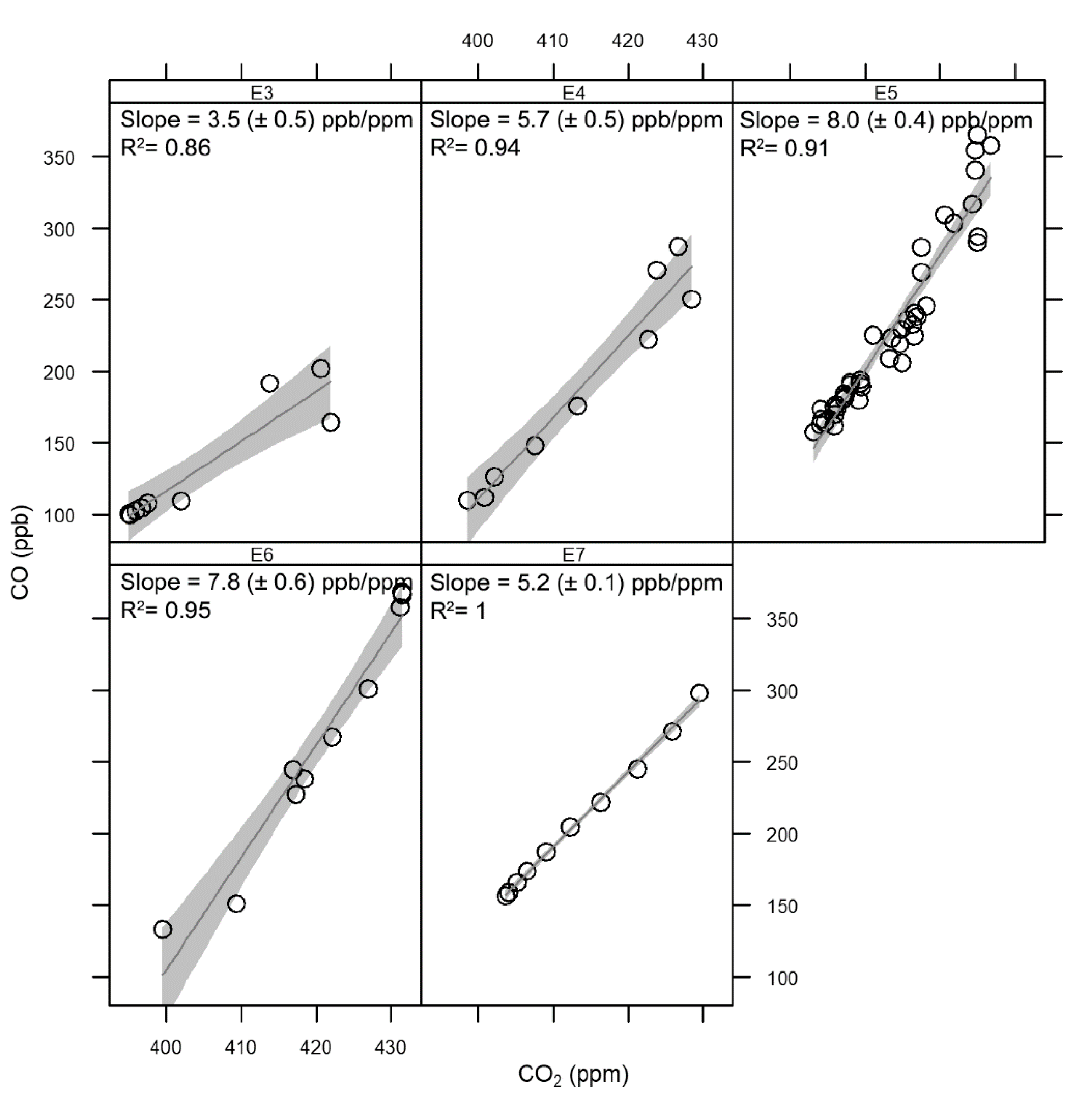
3.2. CO/CO2 Emission Ratios

Figure 4 shows a plot of the CO/CO2 ratios for all individual events except for E1 and E2, for which no CO data were available. The CO/CO2 ratios range between 3.5 and 8.0 ppb/ppm. High coefficients of determination (see Figure 4) support our hypothesis that a considerable part of the CO2 contribution must have been due to combustion of fossil fuels (i.e., gasoline or diesel) and that CO and CO2 were emitted from the same source. Notwithstanding, biogenic CO2 from below and above ground respiration can be transported to the UFS along with anthropogenic CO2, which includes a certain bias to CO and fossil fuel CO2 relations that cannot be excluded.
While comparing our results with those obtained at other sites in Europe, a wide range of emission ratios from fossil fuel emissions was apparent, providing some idea of what to expect for the large-scale European source mix. Table 3 provides a list of some recent studies on CO/CO2 emission ratios for local traffic emissions and fossil fuel combustion. The measured CO/CO2 ratios at the JFJ in February 2009 by Tuzson et al. [9] are of particular interest. The authors studied four distinct pollution events within a month, and the emission ratios ranged from 7.3 to 13.1 ppb/ppm, which are generally higher than ours, except for E5 and E6. The higher values could be due to contributions from biogenic sinks, reducing CO2 while leaving CO unaffected. However, the technological improvement of vehicles with lower CO emissions could explain the lower ratios when comparing the ratio values with studies from previous years (e.g., [23]). Popa et al. [23] measured CO and CO2 close to each end of a highway tunnel in Islisberg, Switzerland, in the year 2011. Vollmer et al. [57] measured emissions at another highway tunnel (Gubrist) in the same region in the year 2004. The values of the year 2011 measurement are almost half of those obtained in the year 2004 [23].

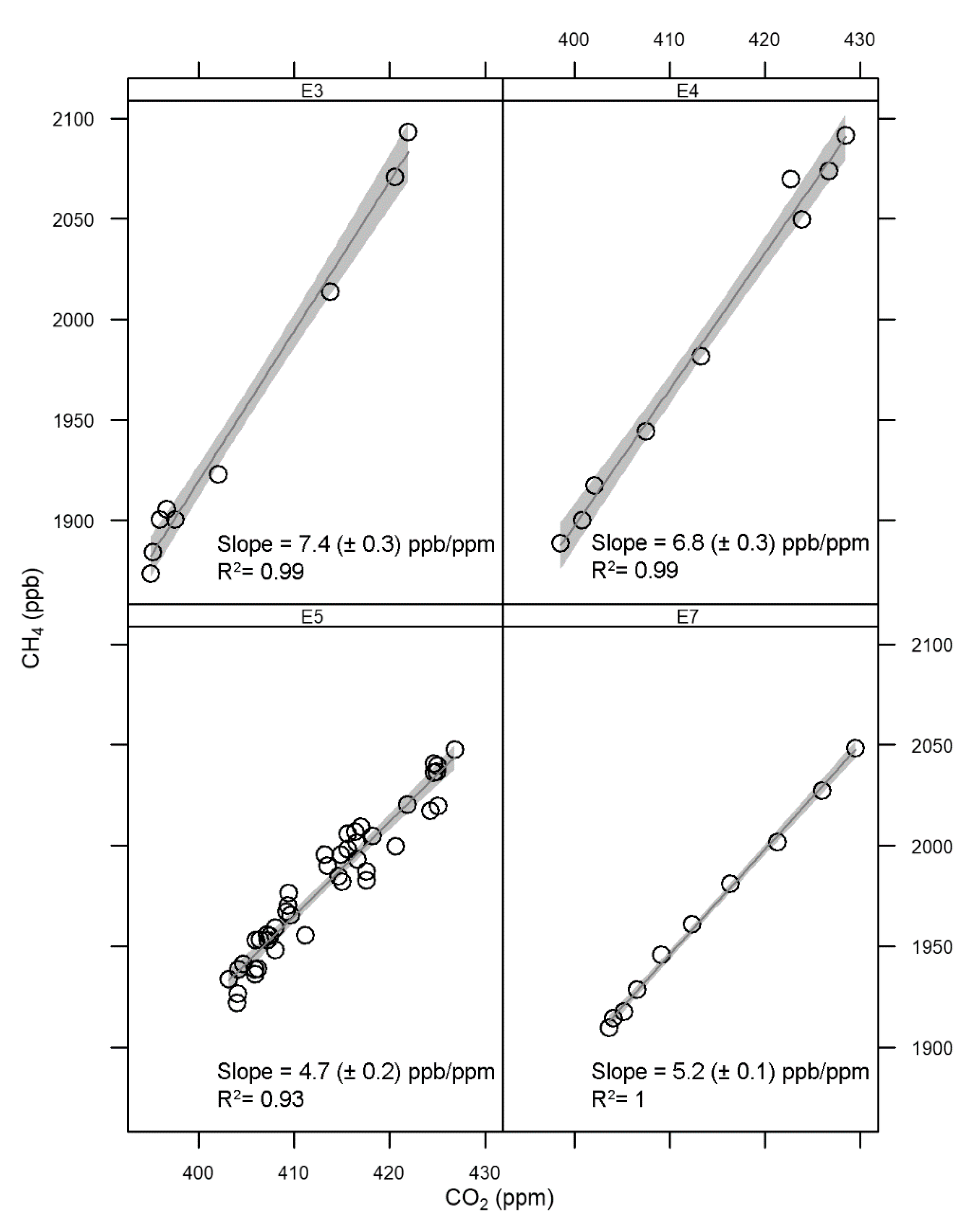
3.3. CH4/CO2 Emission Ratios

Figure 5 shows the observed CH4/CO2 ratios for four events from October 2012 to March 2013 (no CH4 data are available for E1, E2, and E6). The ratios (regression slope) vary from 4.7 to 7.4 ppb/ppm. It was found that emission ratios at the UFS are lower than at other mountain sites that reported 10 to 20 years ago (e.g., the Schauinsland (1205 m a.s.l.), Germany, with a mean ratio of 7.8 ± 1.0 ppb/ppm [52], and the Kasprowy Wierch (1987 m a.s.l.), Poland, with 10.7 ± 0.3 ppm/ppb [51]). Schmidt et al. [52] list a single diurnal cycle of CH4 and CO2 at the JFJ in December 1988, where the emission ratio was 5.3 ± 0.9 ppb/ppm. Worthy et al. [29] observed a decrease in anthropogenic methane emissions in Europe and Siberia from the year 1988 to 2005, which led to low ratios of CH4/CO2. The CH4/CO2 emission ratios obtained in this study compared well with the results of the highway tunnel measurements (4.6 ± 0.2 ppb/ppm) by Popa et al. [23]; indicating local traffic and transport characteristics of the western European vehicle fleet.

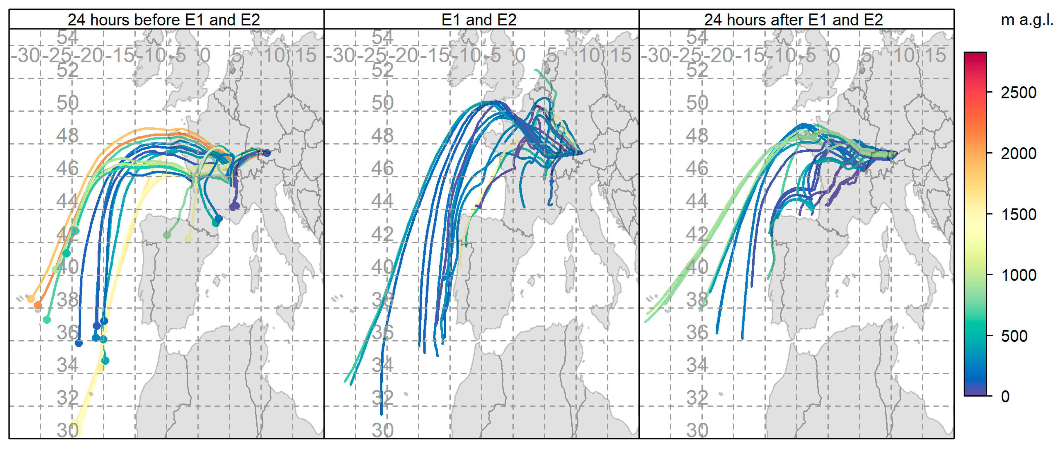
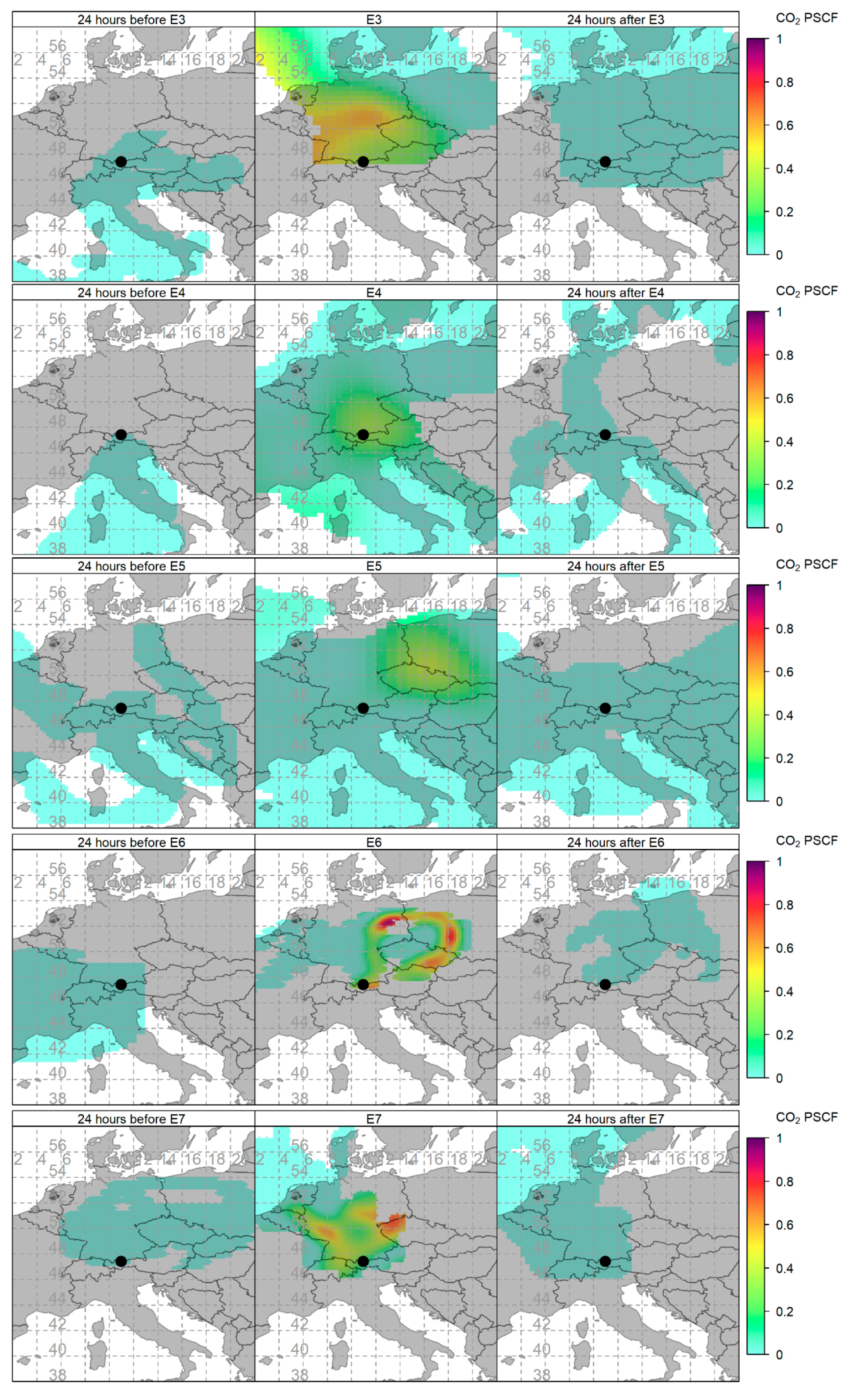
3.4. Backward Trajectories

In order to identify the origin and path followed by the air masses arriving at the UFS during each of the episodes, we merged the hourly output of the HYSPLIT model with the hourly data on atmospheric composition. Figure 6 shows the flow patterns and height of trajectories to the receptor site for E1 and E2. Trajectories are shown in three plots, which contain hourly trajectories of high CO2 mixing ratios during the entire events (middle panel), 24 h before the events (left panel), and 24 h after the events (right panel). Trajectories E1 and E2 are combined due to the short time (4 h) between the two events.
CO2 mixing ratio rapidly increased by 13 ppm in E1 from 397 to 410 ppm, and by 24 ppm in E2 from 399 to 423 ppm, within 5 h and 3 h, respectively. Also, these events were followed by rapid decreases in which the CO2 mixing ratio dropped to 397 ppm within 4 h in E1, and to 397 ppm within 3 h in E2. Moreover, trajectory analysis for E1 and E2, which occurred only 4 h apart, shows no changes in air mass trajectories for 24 h before, during, or 24 h after the events (see Figure 6). Since almost all trajectories flow from the Atlantic Ocean and are assumed to carry clean air, this suggests that the concentration enhancements were caused by regions nearby. Regarding emissions, residential wood burning (mainly in the villages) in the Alpine area is a conventional heating system and a major contributor to CO2 enhancement that fits well with the results of the Keeling plot intercept for E1 and E2 (−24.2‰ and −26.3‰, respectively).
In contrast to E1 and E2, the CO2 mixing ratio increased within 20–91 h and decreased within 9–43 h during the other five events. E3–E7 exhibited short trajectories during the period of the events (CO2 enhancement) from different directions over Europe in which air masses were transported up to the UFS (see Figure S1 in the Supplementary Materials). Trajectories from the 24 h before E6 showed westerly flow patterns in which clean air from the North Atlantic reached the site. Also, trajectories from 24 h after E3 and E7 showed that air masses reached the site via northerly flows from the Arctic Ocean. The case study in [33] is identical to E6 in this study with high formaldehyde, CO, nitrogen oxide, and nitrogen dioxide mixing ratios co-occurring during the event period. Based on the backward trajectory analysis (calculated with HYSPLIT), the influence of polluted PBL was also observed in Leuchner et al. [33], although the trajectories consider neither local wind fields nor complex topography due to the coarse grid resolution of 0.5° of the input model data.
In order to detect the area that most influenced the CO2 mixing ratio, we applied the PSCF to the individual events (except E1 and E2). Figure 7 separately shows the spatial distribution of probable source locations of E3–E7 for 24 h before the events (left panel), during individual events (middle panel), and 24 h after the events (right panel). The coordinates of each map are from 38° to 58° for the latitude with a horizontal resolution of 0.6°. All detected potential sources are located in Germany or at the borders of Germany. This is not unexpected as, according to the European Environment Agency [58], total greenhouse gas emissions per capita in Europe are highest in Germany, where they are mostly associated with energy supply, energy use, and transportation. For more insight, a map of emissions regarding anthropogenic activities is depicted in Figure S2, which was extracted from the EDGAR Ver.432 database relevant to the year 2012. As shown above, E3 and E6 have very similar δ13Cs and, interestingly for these two events, the PSCF maps depict almost the same source area. Though δ13Cs in E4, E5, and E7 are comparable, the detected regions are not quite the same. The detected regions of E4, E5, and E7 partially overlap. However, the detected regions of E7 in the west and east of Germany are very similar to the region detected by Ghasemifard et al. [4]. They showed a PSCF map of wintertime over two and a half years (2012–2014), capturing the CO2 mixing ratio for two specific directions—northwest and northeast of the UFS—where the highest CO2 mixing ratios were measured and most likely linked to coal mining districts in East Germany and industrial regions in northwestern Europe, including the Netherlands and the German Ruhr area. Sturm et al. [59] simulated the isotope signatures of CO2 at the JFJ using a backward Lagrangian model. They showed that short-term variabilities may depend on the origin of the air mass. This suggests that there is a close relationship between atmospheric composition and dominant transported air masses.

4. Conclusions

In this paper, seven events of high CO2 concentration that occurred within five months at the Environmental Research Station Schneefernerhaus (UFS) were investigated. In order to identify and detect pollution events via continuous measurements of CO2 and its stable carbon isotope, selected criteria were adopted for a moving Keeling plot method based on the UFS specifications. Regarding the characterization of the detected events, a combination of four types of information—namely, the δ13Cs signature determined by Keeling plots, CO/CO2 correlation, CH4/CO2 correlation, and back trajectory analysis using the HYSPLIT mode—was employed. We were able to explain the observed short-term variation in atmospheric CO2 mixing ratios by anthropogenic emissions. A summary of the results of the Keeling approaches and emission ratios is provided in Table S1 (Supplementary Materials). The δ13Cs signatures for the most enriched events (E1 and E2) indicated a significant contribution from coal combustion or wood burning, as well as for the other events that exhibited more depleted contributions from natural gas or gasoline. Based on the ratios between CO, CH4, and CO2, it was found that the variation in the atmospheric CO2 mixing ratios was due to the anthropogenic emissions related to road-transport and traffic, which agrees well with δ13C source signature values. The CO/CO2 emission ratio obtained in this research is less than those obtained in previous studies, which is likely due to the technological improvement of vehicles. Though the study period in the cold season minimized the bias of biological activities, it cannot be entirely excluded that biogenic CO2 sources influenced the emission ratios. Back trajectory analysis established source-receptor relationships and revealed that the observed variations in the atmospheric CO2 at the UFS were caused by transport of air masses from Central Europe and Germany (E3–E7), as well as by local influences for two events (E1 and E2).
Even high mountain stations can occasionally measure high CO2 mixing ratios when air masses convey air pollution to these mountain sites. Our analysis revealed that atmospheric trace gas measurements are a vital tool to monitor and quantify air masses that are contaminated by anthropogenic pollution episodes. Measurement of the atmospheric stable isotope ratio 13C/12C and CO2 mixing ratio at high-altitude mountain sites, as well as information about the characteristics of the measurement site, are well suited to the moving Keeling plot for the automatic detection of pollution events. Additional detailed analysis of Foehn episodes, summerly convective upwind systems, and atmospheric circulation using high-resolution meteorological modeling would provide further insights into the investigations of these kinds of events. Besides the potential to clearly explain the differences from free tropospheric conditions, this pollution analysis is an indispensable tool for source contribution, and thus for detection of pollution emissions in the areas surrounding measuring stations.

Supplementary Materials

The following are available online at https://www.mdpi.com/2073-4433/10/6/330/s1. Figure S1: “96-h HYSPLIT backward trajectories (one-hour interval) of air masses reaching UFS during pollution events (E3–E7). For each event, three plots are shown including 24 h before the event (left panel), during the individual event (middle panel), and 24 h after the event (right panel). The color of the trajectories shows the respective height above ground level (m).” Figure S2: “CO2 emission field from anthropogenic sources in 20102. Source: EDGAR V432 emission inventory database (see web site: https://edgar.jrc.ec.europa.eu/overview.php?v=432_GHG).” Table S1: “Summary table of results including the source signatures from the classical and moving Keeling plot and emission ratios of CO/CO2 and CH4/CO2. na are missing values due to missing CO and CH4 data.”

Author Contributions

H.G., F.R.V., J.C., L.R., and A.M. conceptualized the research idea. C.S. and M.L. recorded the data (CO2 and δ13C) and maintained the measurement device, and L.R. provided CH4 and CO data. H.G. performed the data processing with support from S.N.V., Y.Y., and F.R.V. H.G. visualized the backward trajectories with support from M.L. All authors contributed to the interpretation of results and editing of the manuscript.

Acknowledgments

This study was funded by the Virtual Alpine Observatory project of the Bavarian State Ministry of Environment and Consumer Protection. We express our great thanks to the staff and technicians at the UFS for their kind support, especially Rehm and Couret for their essential help, including operation and technical support. We are thankful to the German Environment Agency (Umweltbundesamt, UBA) for access to data and the facilities in their lab. We thank Stephan Hachinger for his important work on the simulations of back trajectories on the Compute Cloud of the Leibniz Supercomputing Centre (LRZ), Garching, Germany.

Conflicts of Interest

The authors declare no conflict of interest. The funding sponsors had no role in the design of the study; in the collection, analyses, or interpretation of data; in the writing of the manuscript, and in the decision to publish the results.

References

  1. IPCC. Contribution of Working Groups I, II and III to the Fifth Assessment Report of the Intergovernmental Panel on Climate Change; IPCC: Geneva, Switzerland, 2014; p. 151. [Google Scholar]
  2. World Meteorological Organization (WMO). Greenhouse Gas Bulletin: The State of Greenhouse Gases in the Atmosphere Based on Global Observations through 2017; WMO: Geneva, Switzerland, 2018. [Google Scholar]
  3. Yuan, Y.; Ries, L.; Petermeier, H.; Steinbacher, M.; Gómez-Peláez, A.J.; Leuenberger, M.C.; Schumacher, M.; Trickl, T.; Couret, C.; Meinhardt, F. Adaptive selection of diurnal minimum variation: A statistical strategy to obtain representative atmospheric CO2 data and its application to European elevated mountain stations. Atmos. Meas. Tech. 2018, 11, 1501–1514. [Google Scholar] [CrossRef]
  4. Ghasemifard, H.; Yuan, Y.; Luepke, M.; Schunk, C.; Chen, J.; Ries, L.; Leuchner, M.; Menzel, A. Atmospheric CO2 and δ13C Measurements from 2012 to 2014 at the Environmental Research Station Schneefernerhaus, Germany: Technical Corrections, Temporal Variations and Trajectory Clustering. Aerosol Air Qual. Res. 2019, 19, 657–670. [Google Scholar] [CrossRef]
  5. Yuan, Y.; Ries, L.; Petermeier, H.; Trickl, T.; Leuchner, M.; Couret, C.; Sohmer, R.; Meinhardt, F.; Menzel, A. On the diurnal, weekly, seasonal cycles and annual trends in atmospheric CO2 at Mount Zugspitze, Germany during 1981–2016. Atmos. Chem. Phys. 2019, 19, 999–1012. [Google Scholar] [CrossRef]
  6. Apadula, F.; Gotti, A.; Pigini, A.; Longhetto, A.; Rocchetti, F.; Cassardo, C.; Ferrarese, S.; Forza, R. Localization of source and sink regions of carbon dioxide through the method of the synoptic air trajectory statistics. Atmos. Environ. 2003, 37, 3757–3770. [Google Scholar] [CrossRef]
  7. Kaiser, A.; Scheifinger, H.; Spangl, W.; Weiss, A.; Gilge, S.; Fricke, W.; Ries, L.; Cemas, D.; Jesenovec, B. Transport of nitrogen oxides, carbon monoxide and ozone to the alpine global atmosphere watch stations Jungfraujoch (Switzerland), Zugspitze and Hohenpeißenberg (Germany), Sonnblick (Austria) and Mt. Krvavec (Slovenia). Atmos. Environ. 2007, 41, 9273–9287. [Google Scholar] [CrossRef]
  8. Uglietti, C.; Leuenberger, M.; Brunner, D. European source and sink areas of CO2 retrieved from Lagrangian transport model interpretation of combined O2 and CO2 measurements at the high alpine research station Jungfraujoch. Atmos. Chem. Phys. 2011, 11, 8017–8036. [Google Scholar] [CrossRef]
  9. Tuzson, B.; Henne, S.; Brunner, D.; Steinbacher, M.; Mohn, J.; Buchmann, B.; Emmenegger, L. Continuous isotopic composition measurements of tropospheric CO2 at Jungfraujoch (3580 m a.s.l.), Switzerland: Real-time observation of regional pollution events. Atmos. Chem. Phys. 2011, 11, 1685–1696. [Google Scholar] [CrossRef]
  10. Ferrarese, S.; Apadula, F.; Bertiglia, F.; Cassardo, C.; Ferrero, A.; Fialdini, L.; Francone, C.; Heltai, D.; Lanza, A.; Longhetto, A. Inspection of high–concentration CO2 events at the Plateau Rosa Alpine station. Atmos. Pollut. Res. 2015, 6, 415–427. [Google Scholar] [CrossRef]
  11. Levin, I.; Graul, R.; Trivett, N.B. Long-term observations of atmospheric CO2 and carbon isotopes at continental sites in Germany. Tellus B 1995, 47, 23–34. [Google Scholar] [CrossRef]
  12. Farquhar, G.D.; Ehleringer, J.R.; Hubick, K.T. Carbon isotope discrimination and photosynthesis. Annu. Rev. Plant Phys. 1989, 40, 503–537. [Google Scholar] [CrossRef]
  13. Mook, W.; Bommerson, J.; Staverman, W. Carbon isotope fractionation between dissolved bicarbonate and gaseous carbon dioxide. Earth Planet Sci. Lett. 1974, 22, 169–176. [Google Scholar] [CrossRef]
  14. Ciais, P.; Tans, P.P.; White, J.W.; Trolier, M.; Francey, R.J.; Berry, J.A.; Randall, D.R.; Sellers, P.J.; Collatz, J.G.; Schimel, D.S. Partitioning of ocean and land uptake of CO2 as inferred by δ13C measurements from the NOAA Climate Monitoring and Diagnostics Laboratory Global Air Sampling Network. J. Geophys. Res. Atm. 1995, 100, 5051–5070. [Google Scholar] [CrossRef]
  15. Pataki, D.E.; Ehleringer, J.R.; Flanagan, L.B.; Yakir, D.; Bowling, D.R.; Still, C.J.; Buchmann, N.; Kaplan, J.O.; Berry, J.A. The application and interpretation of Keeling plots in terrestrial carbon cycle research. Global Biogeochem. Cycles 2003, 17. [Google Scholar] [CrossRef] [Green Version]
  16. Pang, J.; Wen, X.; Sun, X. Mixing ratio and carbon isotopic composition investigation of atmospheric CO2 in Beijing, China. Sci. Total Environ. 2016, 539, 322–330. [Google Scholar] [CrossRef] [PubMed]
  17. Pataki, D.E.; Xu, T.; Luo, Y.Q.; Ehleringer, J. Inferring biogenic and anthropogenic carbon dioxide sources across an urban to rural gradient. Oecologia 2007, 152, 307–322. [Google Scholar] [CrossRef]
  18. Wada, R.; Pearce, J.K.; Nakayama, T.; Matsumi, Y.; Hiyama, T.; Inoue, G.; Shibata, T. Observation of carbon and oxygen isotopic compositions of CO2 at an urban site in Nagoya using Mid-IR laser absorption spectroscopy. Atmos. Environ. 2011, 45, 1168–1174. [Google Scholar] [CrossRef]
  19. Pfister, G.; Petron, G.; Emmons, L.K.; Gille, J.C.; Edwards, D.P.; Lamarque, J.-F.; Attie, J.-L.; Granier, C.; Novelli, P.C. Evaluation of CO simulations and the analysis of the CO budget for Europe. J. Geophys. Res. Atm. 2004, 109. [Google Scholar] [CrossRef]
  20. Levin, I.; Karstens, U. Inferring high-resolution fossil fuel CO2 records at continental sites from combined 14CO2 and CO observations. Tellus B 2007, 59, 245–250. [Google Scholar] [CrossRef]
  21. Vardag, S.N.; Gerbig, C.; Janssens-Maenhout, G.; Levin, I. Estimation of continuous anthropogenic CO2: Model-based evaluation of CO2, CO, δ13C(CO2) and Δ14C(CO2) tracer methods. Atmos. Chem. Phys. 2015, 15, 12705–12729. [Google Scholar] [CrossRef]
  22. Vogel, F.; Hammer, S.; Steinhof, A.; Kromer, B.; Levin, I. Implication of weekly and diurnal 14C calibration on hourly estimates of CO-based fossil fuel CO2 ata moderately polluted site in southwestern Germany. Tellus B 2010, 62, 512–520. [Google Scholar] [CrossRef]
  23. Popa, M.E.; Vollmer, M.K.; Jordan, A.; Brand, W.A.; Pathirana, S.L.; Rothe, M.; Röckmann, T. Vehicle emissions of greenhouse gases and related tracers from a tunnel study: CO: CO2, N2O: CO2, CH4: CO2, O2: CO2 ratios, and the stable isotopes 13C and 18O in CO2 and CO. Atmos. Chem. Phys. 2014, 14, 2105–2123. [Google Scholar] [CrossRef]
  24. Schmidt, A.; Rella, C.W.; Göckede, M.; Hanson, C.; Yang, Z.; Law, B.E. Removing traffic emissions from CO2 time series measured at a tall tower using mobile measurements and transport modeling. Atmos. Environ. 2014, 97, 94–108. [Google Scholar] [CrossRef]
  25. Thom, M.; Bösinger, R.; Schmidt, M.; Levin, I. The regional budget of atmospheric methane of a highly populated area. Chemosphere 1993, 26, 143–160. [Google Scholar] [CrossRef]
  26. Nam, E.K.; Jensen, T.E.; Wallington, T.J. Methane emissions from vehicles. Environ. Sci. Technol. 2004, 38, 2005–2010. [Google Scholar] [CrossRef] [PubMed]
  27. Nakagawa, F.; Tsunogai, U.; Komatsu, D.D.; Yamada, K.; Yoshida, N.; Moriizumi, J.; Nagamine, K.; Iida, T.; Ikebe, Y. Automobile exhaust as a source of 13C-and D-enriched atmospheric methane in urban areas. Org. Geochem. 2005, 36, 727–738. [Google Scholar] [CrossRef]
  28. Tohjima, Y.; Kubo, M.; Minejima, C.; Mukai, H.; Tanimoto, H.; Ganshin, A.; Maksyutov, S.; Katsumata, K.; Machida, T.; Kita, K. Temporal changes in the emissions of CH4 and CO from China estimated from CH4/CO2 and CO/CO2 correlations observed at Hateruma Island. Atmos. Chem. Phys. 2014, 14, 1663–1677. [Google Scholar] [CrossRef]
  29. Worthy, D.E.; Chan, E.; Ishizawa, M.; Chan, D.; Poss, C.; Dlugokencky, E.J.; Maksyutov, S.; Levin, I. Decreasing anthropogenic methane emissions in Europe and Siberia inferred from continuous carbon dioxide and methane observations at Alert, Canada. J. Geophys. Res. 2009, 114. [Google Scholar] [CrossRef] [Green Version]
  30. Fang, S.-X.; Luan, T.; Zhang, G.; Wu, Y.-L.; Yu, D.-J. The determination of regional CO2 mole fractions at the Longfengshan WMO/GAW station: A comparison of four data filtering approaches. Atmos. Environ. 2015, 116, 36–43. [Google Scholar] [CrossRef]
  31. Henne, S.; Brunner, D.; Folini, D.; Solberg, S.; Klausen, J.; Buchmann, B. Assessment of parameters describing representativeness of air quality in-situ measurement sites. Atmos. Chem. Phys. 2010, 10, 3561–3581. [Google Scholar] [CrossRef] [Green Version]
  32. Gantner, L.; Hornsteiner, M.; Egger, J.; Hartjenstein, G. The diurnal circulation of Zugspitzplatt: Observations and modeling. Meteorol. Z. 2003, 12, 95–102. [Google Scholar] [CrossRef]
  33. Leuchner, M.; Ghasemifard, H.; Lüpke, M.; Ries, L.; Schunk, C.; Menzel, A. Seasonal and diurnal variation of formaldehyde and its meteorological drivers at the GAW site Zugspitze. Aerosol Air Qual. Res. 2016, 16, 801–815. [Google Scholar] [CrossRef]
  34. Zellweger, C.; Forrer, J.; Hofer, P.; Nyeki, S.; Schwarzenbach, B.; Weingartner, E.; Ammann, M.; Baltensperger, U. Partitioning of reactive nitrogen (NOy) and dependence on meteorological conditions in the lower free troposphere. Atmos. Chem. Phys. 2003, 3, 779–796. [Google Scholar] [CrossRef]
  35. GAWSIS. Station Information System. Available online: https://gawsis.meteoswiss.ch/GAWSIS/ (accessed on 17 June 2019).
  36. Nara, H.; Tanimoto, H.; Tohjima, Y.; Mukai, H.; Nojiri, Y.; Katsumata, K.; Rella, C.W. Effect of air composition (N2, O2, Ar, and H2O) on CO2 and CH4 measurement by wavelength-scanned cavity ring-down spectroscopy: Calibration and measurement strategy. Atmos. Meas. Tech. 2012, 5, 2689–2701. [Google Scholar] [CrossRef]
  37. Pang, J.; Wen, X.; Sun, X.; Huang, K. Intercomparison of two cavity ring-down spectroscopy analyzers for atmospheric 13CO2/12CO2 measurement. Atmos. Meas. Tech. 2016, 9, 3879–3891. [Google Scholar] [CrossRef]
  38. Rella, C.W.; Chen, H.; Andrews, A.E.; Filges, A.; Gerbig, C.; Hatakka, J.; Karion, A.; Miles, N.L.; Richardson, S.J.; Steinbacher, M.; et al. High accuracy measurements of dry mole fractions of carbon dioxide and methane in humid air. Atmos. Meas. Tech. 2013, 6, 837–860. [Google Scholar] [CrossRef] [Green Version]
  39. Vogel, F.R.; Huang, L.; Ernst, D.; Giroux, L.; Racki, S.; Worthy, D.E. Evaluation of a cavity ring-down spectrometer for in situ observations of 13CO2. Atmos. Meas. Tech. 2013, 6, 301–308. [Google Scholar] [CrossRef]
  40. Wen, X.-F.; Meng, Y.; Zhang, X.-Y.; Sun, X.-M.; Lee, X. Evaluating calibration strategies for isotope ratio infrared spectroscopy for atmospheric 13CO2/12CO2; measurement. Atmos. Meas. Tech. 2013, 6, 1491–1501. [Google Scholar] [CrossRef]
  41. Team, R. RStudio: Integrated Development for R; R Studio Inc.: Boston, MA, USA, 2016; Available online: http://www.rstudio.com/ (accessed on 7 March 2019).
  42. Carslaw, D.C.; Ropkins, K. Openair—An R package for air quality data analysis. Environ. Modell. Softw. 2012, 27, 52–61. [Google Scholar] [CrossRef]
  43. Wickham, H. GGPLOT2: Elegant Graphics for Data Analysis; Springer: New York, NY, USA, 2010. [Google Scholar]
  44. Keeling, C.D. The concentration and isotopic abundances of atmospheric carbon dioxide in rural areas. Geochim. Cosmochim. Acta 1958, 13, 322–334. [Google Scholar] [CrossRef]
  45. Keeling, C.D. The concentration and isotopic abundances of carbon dioxide in rural and marine air. Geochim. Cosmochim. Acta 1961, 24, 277–298. [Google Scholar] [CrossRef]
  46. Vardag, S.N.; Hammer, S.; Levin, I. Evaluation of 4 years of continuous 13C(CO2) data using a moving Keeling plot method. Biogeosciences 2016, 13, 4237–4251. [Google Scholar] [CrossRef]
  47. Miller, J.B.; Tans, P.P. Calculating isotopic fractionation from atmospheric measurements at various scales. Tellus B 2003, 55, 207–214. [Google Scholar] [CrossRef]
  48. Krystek, M.; Anton, M. A weighted total least-squares algorithm for fitting a straight line. Meas. Sci. Tech. 2007, 18, 3438. [Google Scholar] [CrossRef]
  49. Ammoura, L.; Xueref-Remy, I.; Gros, V.; Baudic, A.; Bonsang, B.; Petit, J.-E.; Perrussel, O.; Bonnaire, N.; Sciare, J.; Chevallier, F. Atmospheric measurements of ratios between CO2 and co-emitted species from traffic: A tunnel study in the Paris megacity. Atmos. Chem. Phys. 2014, 14, 12871–12882. [Google Scholar] [CrossRef]
  50. Xueref-Remy, I.; Messager, C.; Filippi, D.; Pastel, M.; Nedelec, P.; Ramonet, M.; Paris, J.D.; Ciais, P. Variability and budget of CO2 in Europe: Analysis of the CAATER airborne campaigns—Part 1: Observed variability. Atmos. Chem. Phys. 2011, 11, 5655–5672. [Google Scholar] [CrossRef]
  51. Necki, J.; Schmidt, M.; Rozanski, K.; Zimnoch, M.; Korus, A.; Lasa, J.; Graul, R.; Levin, I. Six-year record of atmospheric carbon dioxide and methane at a high-altitude mountain site in Poland. Tellus B 2003, 55, 94–104. [Google Scholar] [CrossRef]
  52. Schmidt, M.; Graul, R.; Sartorius, H.; Levin, I. Carbon dioxide and methane in continental Europe: A climatology, and 222Radon-based emission estimates. Tellus B 1996, 48, 457–473. [Google Scholar] [CrossRef]
  53. Draxler, R.R.; Hess, G.D. An overview of the HYSPLIT_4 modelling system for trajectories, dispersion and deposition. Aust. Met. Mag. 1998, 47, 295–308. [Google Scholar]
  54. Stohl, A. Trajectory statistics—A new method to establish source-receptor relationships of air pollutants and its application to the transport of particulate sulfate in Europe. Atmos. Environ. 1996, 30, 579–587. [Google Scholar] [CrossRef]
  55. Ashbaugh, L.L.; Malm, W.C.; Sadeh, W.Z. A residence time probability analysis of sulfur concentrations at Grand Canyon National Park. Atmos. Environ. 1985, 19, 1263–1270. [Google Scholar] [CrossRef]
  56. Seinfeld, J.H.; Pandis, S.N. Atmospheric Chemistry and Physics: From Air Pollution to Climate Change, 3rd ed.; John Wiley & Sons: Hoboken, NJ, USA, 2016. [Google Scholar]
  57. Vollmer, M.K.; Juergens, N.; Steinbacher, M.; Reimann, S.; Weilenmann, M.; Buchmann, B. Road vehicle emissions of molecular hydrogen (H2) from a tunnel study. Atmos. Environ. 2007, 41, 8355–8369. [Google Scholar] [CrossRef]
  58. European Environment Agency. Greenhouse Gas Emission Trends and Projections in Europe 2012; European Environment Agency: Copenhagen, Denmark, 2012. [Google Scholar]
  59. Sturm, P.; Tuzson, B.; Henne, S.; Emmenegger, L. Tracking isotope signatire of CO2 at the high altitude site Jungfraujoch with laser spectroscopy: Analytical improvements and respective results. Atmos. Meas. Tech. 2013, 6, 1659–1671. [Google Scholar] [CrossRef]
Figure 1. Source signature determination using the Keeling plot. (a) The CO2 mixing ratio (solid line) and δ13C (dashed line) of event E7, and (b) the Keeling plot for the entire event as shown in (a). The y-intercept and coefficient of determination R2 of the fitted linear regressions following Equation (3) are given in (b).
Atmosphere 10 00330 g001
Figure 2. Temporal variation of the mixing ratios of CO2, CO, and CH4, as well as the stable carbon isotope ratio of atmospheric CO213C), for five months at the Environmental Research Station Schneefernerhaus (UFS). The arrows point to the studied episodes labeled E1–E7. The shaded areas indicate distinct pollution events (the first event actually contains separate two events, but due to the short period between them the shaded area is shown as a single event).
Atmosphere 10 00330 g002
Figure 3. Intercepts of Keeling plots (δs) during the individual pollution events. (a) Results of the classical Keeling plot method. Black circles indicate the intercept and the error bars show the error of the intercept. (b) Results of moving the Keeling plot method depicted as box plots. The whiskers of the boxplots indicate the minimum and maximum values, the lower and upper boundaries of the boxes are the 25th- and 75th-percentiles, and the horizontal lines inside boxes represent medians.
Atmosphere 10 00330 g003
Figure 4. Linear regressions of the hourly mean mixing ratios of CO and CO2 for the five pollution events E3–E7 (CO data not available for E1 and E2). The slope and coefficient of determination R2 are given. The shaded areas around the regression lines represent the range in which the true regression line lies at a certain level of confidence (95% in the plot). The slope of the regressions corresponds to CO/CO2 emission ratios.
Atmosphere 10 00330 g004
Figure 5. Linear regressions of hourly mean mixing ratios of CH4 and CO2 for four pollution events (CH4 data not available for E1, E2, and E6). The slope and coefficient of determination R2 are given. The shaded areas around the regressions line represent the range in which the true regression line lies at a certain level of confidence (95% in the plot). The slope of the regressions corresponds to CH4/CO2 emission ratios.
Atmosphere 10 00330 g005
Figure 6. HYSPLIT backward trajectories (1-h interval) of air masses reaching the UFS during pollution events E1 and E2. The three plots are 24 h before the events (left panel), E1 and E2 combined during the events (middle panel), and 24 h after the events (right panel). The color of the trajectories shows the respective height above ground level (m).
Atmosphere 10 00330 g006
Figure 7. Potential source contribution function (PSCF) plot of CO2. The color of the maps shows the respective probabilities. For each event (E3 to E7), three plots are shown including 24 h before the event, during the event, and 24 h after the event (left, center, and right, respectively). Blue to purple colors (0 ≤ Pij ≤ 1) identify regions from which elevated CO2 potentially originated. Black circles show the position of the UFS study site.
Atmosphere 10 00330 g007
Table 1. Filter criteria and rationale based on Vardag et al. [46].
Filter CriteriaRationale
Monotonous CO2 increase over 5 hReasons for a decrease could be a simultaneously occurring sink or a boundary layer break-up, both hurting the prerequisites of a Keeling plot.
Error of intercept < 2‰Changes of mean source mix due to change of emission characteristics, background or footprint area show a non-linear behavior in a Keeling plot. Thus, choosing a maximum error of the intercept, δS of <2‰, can filter out these situations.
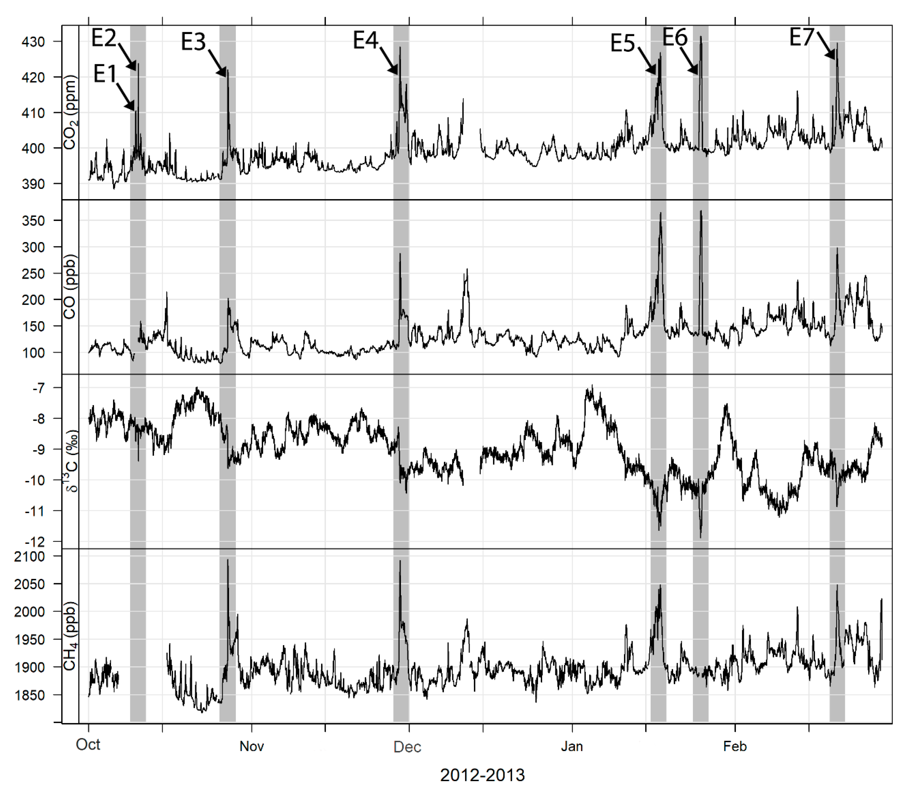
Table 2. Date and duration of investigated episodes.
EpisodeDayMonth-YearTotal Duration (h)Duration until the Maximum of CO2 (h)
E10910-201295
E21010-201263
E327–2810-2012259
E428–3011-2012629
E515–1801-20139143
E62501-20132010
E719–2102-20134210
Table 3. CO/CO2 emission ratios for traffic and anthropogenic emissions in Europe.
ReferenceCO/CO2
(ppb/ppm)
LocationEnvironmentYear
Vollmer at al. (2007) [57]9.19 ± 3.74Switzerlandtunnel2004
Vogel et al. (2010) [22]13.5 ± 2.5Germanycity2002–2009
Tuzson et al. (2011) [9]9.35 ± 2.66Switzerlandremote site2009
Popa et al. (2014) [23]4.15 ± 0.34Switzerlandtunnel2011
Ammoura et al. (2014) [49]5.68 ± 2.43Francetunnel2012
This study6.02 ± 0.12Germanyremote site2012–2013

