Marginal Benefit to South Asian Economies from SO₂ Emissions Mitigation and Subsequent Increase in Monsoon Rainfall

Abstract

Sulphate aerosols are dominated by SO₂ emissions from coal-burning for the Indian electricity sector and they are thought to have a short term but significant, negative impact on South Asian Summer Monsoon rainfall. This reduction in precipitation in turn can lead to reduced economic outputs, primarily through smaller agricultural yields. By bringing together estimates of (a) the impact of sulphate aerosols on precipitation and (b) the observed relationship between monsoon rainfall and GDP, we present a methodology to estimate the possible financial cost of this effect on the Indian economy and on its agricultural sector. Our preliminary estimate is that the derived benefits could be large enough that around 50% of India’s SO₂ emissions could be economically mitigated at no cost or net benefit, although it should be noted that the large uncertainties in the underlying relationships mean that the overall uncertainty is also large. Comparison of the 1952–1981 and 1982–2011 periods indicates that the Indian economy may now be more resilient to variability of the monsoon rainfall. As such, a case could be made for action to reduce SO₂ emissions, particularly in the crucial monsoon period. This would have a significant, positive effect on a crucial and large sector in India’s economy and the effects would be visible almost instantly. The recent growth in renewable energy sources in India and the consequent, reduced increase in coal burning means that further financial costs have already been avoided. This impact should be further investigated so that it can be included in cost-benefit analyses of different fuel types in the region. The significant uncertainties associated with these calculations are discussed.

1. Introduction

The South Asian summer monsoon provides 80% of annual precipitation to around a billion people [1]. The main rainy season runs from June to September, though there are significant interannual variations. The strong seasonal character of the monsoon results from the large-scale thermal contrast arising from the differing oceanic and terrestrial heat capacities and their response to the seasonal variation in the solar radiation, although dynamical as well as thermodynamical drivers must be considered [1,2]. Models suggest that the presence of greenhouse gases alone and the associated warming of the atmosphere would tend to cause an increase in monsoon rainfall [3].

Aerosols (anthropogenic and natural, such as sulphate, dust and black carbon) influence the course of the monsoon each year, either through their radiative influence on atmospheric motions or through their impact on cloud nucleation, cloud droplet size and rainfall rates [1,3,4,5,6,7]. In general, increased aerosols are thought to decrease the monsoon rainfall. This is in contrast to the increase in monsoon rainfall that is calculated to occur as a result of increased greenhouse gases alone. Over the past decades, the long-term reduction in summer monsoon rainfall is therefore attributed to the impact of the long-term increase in anthropogenically induced aerosols being larger than the influence of the increased greenhouse gases. The impact of aerosols is felt on shorter time-scales—from weeks to years—and depends critically on the physical and chemical characteristics of the aerosol under consideration [8].

The aerosol abundance in the atmosphere has increased along with the growth in the economy and the use of fossil fuels. Sulphate aerosols, resulting principally from the burning of coal, are a major fraction of the total aerosol abundance. Other important categories include: black carbon from incomplete fuel burning; dust from wind disturbance of surface terrain; and bioaerosol (pollen, spores, etc.). The different categories have different effects on the monsoon and its rainfall and complex atmospheric models are required to diagnose the effects of particular aerosol types. Locally produced aerosols are thought to be the larger influence on the monsoon precipitation while remotely produced aerosols have more influence on the monsoon timing and circulation [9,10] (see Section 2.1 for further discussion).

Agriculture, which is a major occupation in the region, depends heavily on the monsoon rains and their timing. High rainfall is generally associated with higher grain yield and vice versa [11]. The long-term decrease in rainfall is thus of considerable importance to individuals and to governments. In India, agriculture comprises 25–30% of the country’s economy and roughly 65% of the population is rural and dependent on agriculture-related activities. From 1979 to 1992, per capita food production grew at ~1.6% per year—and it could have grown faster if rainfall had not decreased in the same period [11].

In this paper, we describe a methodology to calculate the financial impact of sulphate aerosols on the Indian economy and we present our preliminary estimates. This approach involves pulling together information from several fields (atmospheric science, agriculture and economics), each of which has large uncertainties. The methodology developed is described in Section 2 and the preliminary results are presented in Section 3. The main findings, the associated uncertainties and the possible implications for policy are discussed in Section 4. Finally, Section 5 summarises the findings as well as some areas of possible further work.

2. Methodology

This paper presents a methodology to estimate the marginal benefit to South Asian economies from reducing SO₂ emissions. Agriculture plays an important role in South Asian economies. SO₂ emissions promote aerosol formation, which could reduce the monsoon rainfall and so harm the agricultural yields. The reduction of SO₂ emissions could provide net benefit on agricultural and thus the economies in South Asia. In this paper, such benefit is calculated in form of a marginal benefit of SO₂ emissions mitigation.

The methodology is based on two relationships. The first is the relationship between SO₂ emissions and changes (reductions) in rainfall. The second relationship is between Indian Summer Monsoon Rainfall (henceforth ISMR) and the Indian economy, henceforth the Economic Influence of Rainfall (EIR). By combining these two relationships, it is possible to establish a relationship between SO₂ emissions and the economy. Other economic impacts, such as human health and crop damage with reduced yields from exposure to SO₂ are not included in this calculation, although they are briefly addressed in the discussion section.

2.1. Relationship between SO₂ Emissions and Indian Summer Monsoon Rainfall

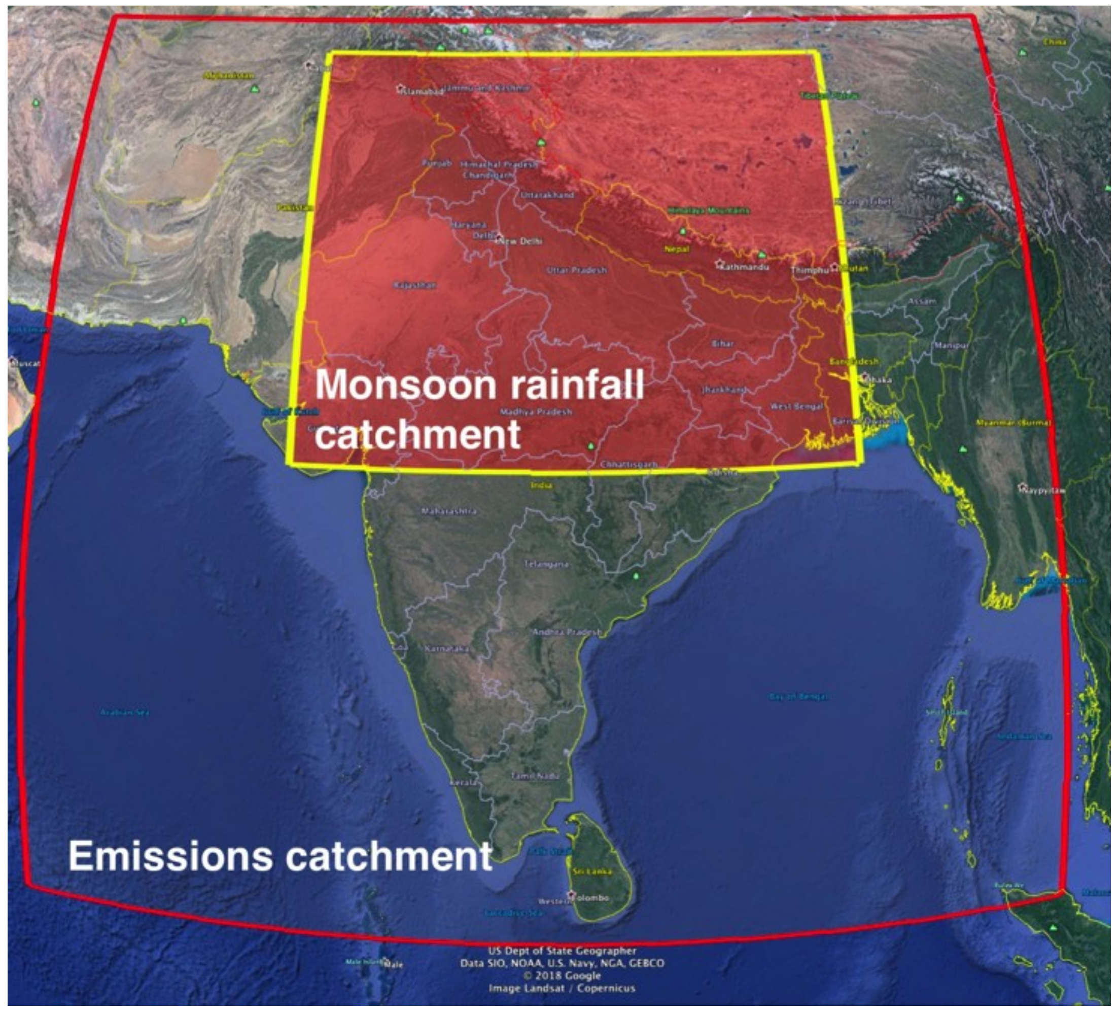
CMIP5 (Fifth Coupled Model Intercomparison Project) is “… a standard experimental protocol for studying the output of coupled atmosphere-ocean general circulation models (AOGCMs). CMIP provides a community-based infrastructure in support of climate model diagnosis, validation, intercomparison, documentation and data access. … Virtually the entire international climate modeling community has participated in this project since its inception in 1995.” [12]. Guo et al. [13] use historic CMIP5 experiments to compare the impact of the increased radiative forcing from greenhouse gases with that of anthropogenic aerosols on the South Asian monsoon. They additionally assess the role of direct and indirect aerosol effects and discuss the implications for future projections of monsoon rainfall. As part of this analysis, they present results for model experiments in which sulphate levels are reduced from present day levels (1976–2005) to pre-industrial levels (1860) for (a) ‘India’ and (b) the rest of the world (‘RoW’). Figure 1 shows the two relevant catchment areas for this analysis as defined by Guo et al. [12]: the area which is considered ‘India’ for SO₂ emissions (5.0°–36.25°N, 60.0°–97.50°E) and the area in which the changes in ISMR are measured (21°–35°N, 70°–90°E). We use these areas in our analysis to avoid introducing additional uncertainties due to scaling the area-averaged impacts from Guo et al. [12] to different areas.

The effects of these emissions scenarios on rainfall are shown in

Table 1. Change in daily and seasonal rainfall during the June–September monsoon season calculated for various SO₂ emissions scenarios of South Asia and for the rest of the world (RoW) from Guo et al. [13] (p. 6952). The percentage refers to the JJAS aggregate deviation compared to the seasonal average aggregate rainfall from [15] (4887).

Average Rainfall Deviation in June-September Period	SO2 Emissions Scenario
	S. Asia: Present Day RoW: Present Day	S. Asia: Preindustrial RoW: Present Day
Daily (mm)	−0.88	−0.73
JJAS aggregate (mm)	−107	−89
JJAS aggregate (%)	−13%	−11%

. Global, present-day SO₂ emissions are found to decrease the ISMR by 107 mm per season (June–September-JJAS) compared to preindustrial (1860) levels, a 13% reduction from the average level of 852 mm [15], with one quarter of the effect coming from South Asian emissions [13]. If SO₂ emissions from only South Asia (represented by the emissions catchment box in Figure 1) were reduced to preindustrial levels, while the rest of the world’s emissions (i.e., all those outside the catchment in Figure 1) are maintained at present-day levels, ISMR would be diminished by 89 mm per season (11% of the historical average). By extension, we deduce that if South Asian emissions were reduced to preindustrial level (zero) while all others are maintained at current levels, there would be an increase in ISMR of 18 mm (107 mm–89 mm or 2.2% of the 852 mm historical average) from the present day level.

Other authors have examined the effect of similar emission scenarios on local rainfall patterns and volumes. Ganguly et al. [5,5] examine an emission scenario of “anthropogenic” aerosol emissions at pre-industrial (i.e., very low to zero) levels over Asia and present day levels in the rest of the world and find an annual mean reduction in rainfall of 0.1 mm/day (The catchment area for rainfall in this case is a box: 0°–60°N and 60°E–150°E.). They conclude that most of the observed reduction in precipitation over India is caused by locally emitted aerosols from anthropogenic activities rather than from emissions from remote activities. Bollasina et al. [9] use scenarios consisting of emissions of SO₂, black carbon and organic carbon and find that both local and remote aerosols are effective in reducing precipitation over India, with the former exerting the predominant impact. These and other [4,15] studies support the thesis of anthropogenic emissions causing a reduction of ISMR with a greater proportion of the total effect attributable to local emissions, in contrast to the findings of Guo et al. [13], who find the larger effect to come from non-local emissions. If local emissions do indeed have a greater effect than non-local emissions, the calculated benefit of emissions mitigation would be proportionally greater. In other words the assumption used here is conservative as Guo et al. [12] find a greater proportion of the total effect of emissions is attributable to non-local emissions. Furthermore, the aim of this study is to find effects with clear policy implications, so Guo et al.’s examination of SO₂ in isolation [13] is the most appropriate as disaggregating the sources of emissions is beyond the scope of this study. As suggested by Bollasina et al. [4], there is a nonlinear response to the scenarios of emissions they examine. However no information is provided for the nature of the non-linearity of response. In the absence of better information, the authors adopted the conservative assumption is that the relationship between SO₂ emissions and ISMR is linear (between the points represented by the present day and South Asian preindustrial scenarios), that is, that for a given proportion of emissions reduction, the same proportion of effect in ISMR is observed. It is likely that co-emissions with SO₂ (e.g., black carbon) have additional effects on ISMR but this is not investigated here due to the lack of sufficient, relevant information.

2.2. Relationship between Indian Summer Monsoon Rainfall and The Economy

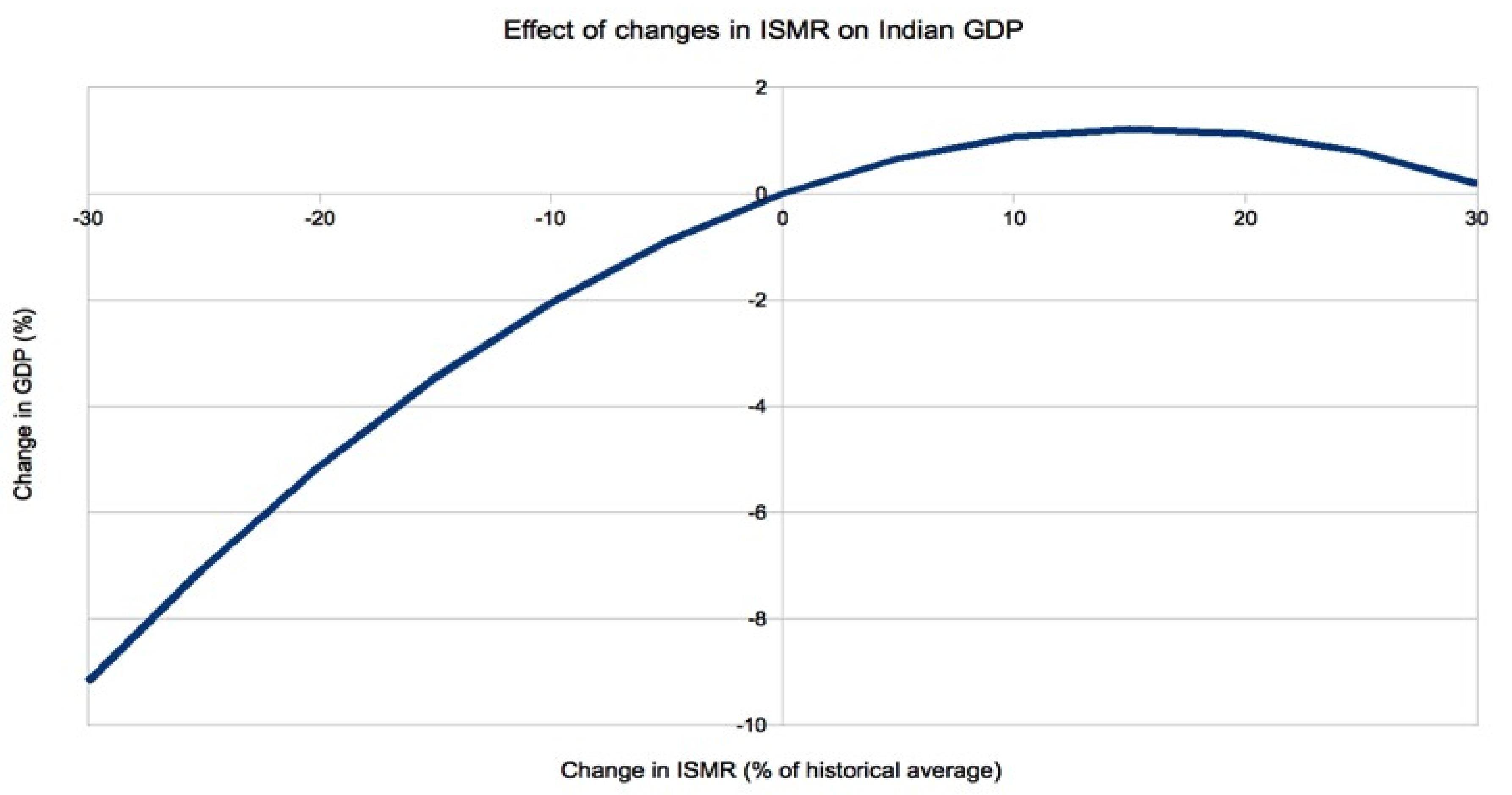
The second crucial relationship to define is that between ISMR and the economy. Gadgil and Gadgil [15] (p. 4892) provide this relationship from their study of the observed variation of ISMR and Indian GDP for the years 1951–2003. Their study assumes a quadratic dependence as in the following equation and their results are presented as a graph in Figure 2:

IGDP = a × AnomISMR² + b × AnomISMR

IGDP is the percentage change in India’s GDP (as a %) and AnomISMR is the deviation (in %) of ISMR from the historical average, a = −0.005 and b = 0.1565.

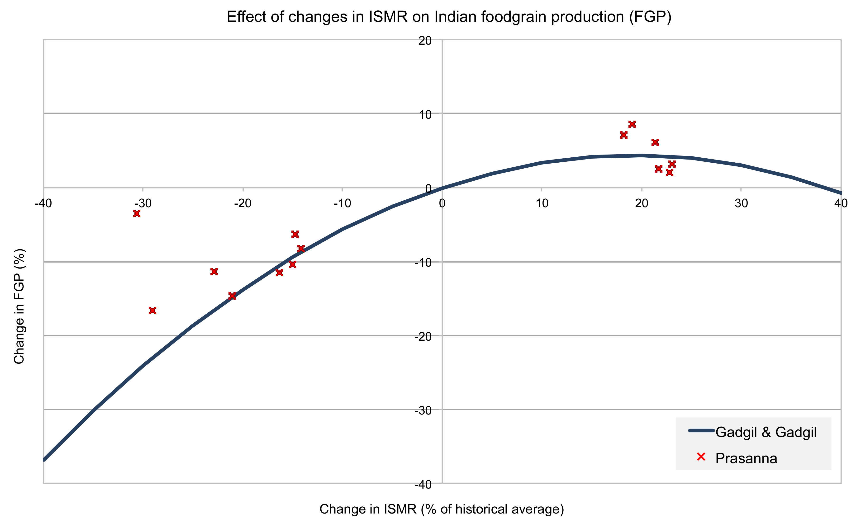
Gadgil and Gadgil [14] assume that the EIR is a result of rainfall’s effect on Food Grain Production (FGP) and perform a similar analysis on this relationship to that for ISMR and GDP. They find a similarly shaped function, shown in Figure 3. Prasanna [11] performs a similar analysis, examining only particularly dry or wet years for the years 1966–2010, their data are also plotted in Figure 3.

As Figure 3 shows, the two analyses are a good visual fit, strengthening the case for the relationship found by Gadgil and Gadgil [14] between ISMR and FGP and indirectly for their posited relationship between ISMR and Indian GDP.

Updated ISMR-GDP Analysis

Gadgil and Gadgil’s analysis uses data until 2003. An updated analysis is performed here to investigate the effects of India’s rapid rate of economic growth and in particular whether agriculture’s contribution to the overall economy has decreased. Further, since India is responsible for the bulk of the SO₂ emissions and is most affected economically, a second analysis is performed for India only. Data for monthly rainfall are for the years 1901 until 2014 [16] and GDP (in 2004–05 prices) data are from [17] for the financial years (The Indian financial year runs from the 1st of April until the 31st of March, so the GDP figures have been adjusted to reflect a calendar year.) 1951–52 until 2011–12 for the whole Indian economy (‘All-India’) and for the subsector ‘agricultural sector and allied services’. No official definition of what is included in ‘Agriculture and allied services’ could be found but it is listed as “including agriculture, livestock, forestry and fishery” [18] and other official documentation includes in it the outputs agriculture and livestock and inputs such as fertilisers and pesticides, livestock feed, fuel and irrigation costs, amongst others [19].). Both the agricultural sector and the whole economy are examined as while it is assumed that the primary driver of the EIR is rainfall’s effect on crop-yields and the agricultural sector, there is likely to be a follow-on effect on the whole economy. This is done for the periods, 1952–2011, 1952–1981, 1982–2011 and 1952–2003 (for comparison with Gadgil).

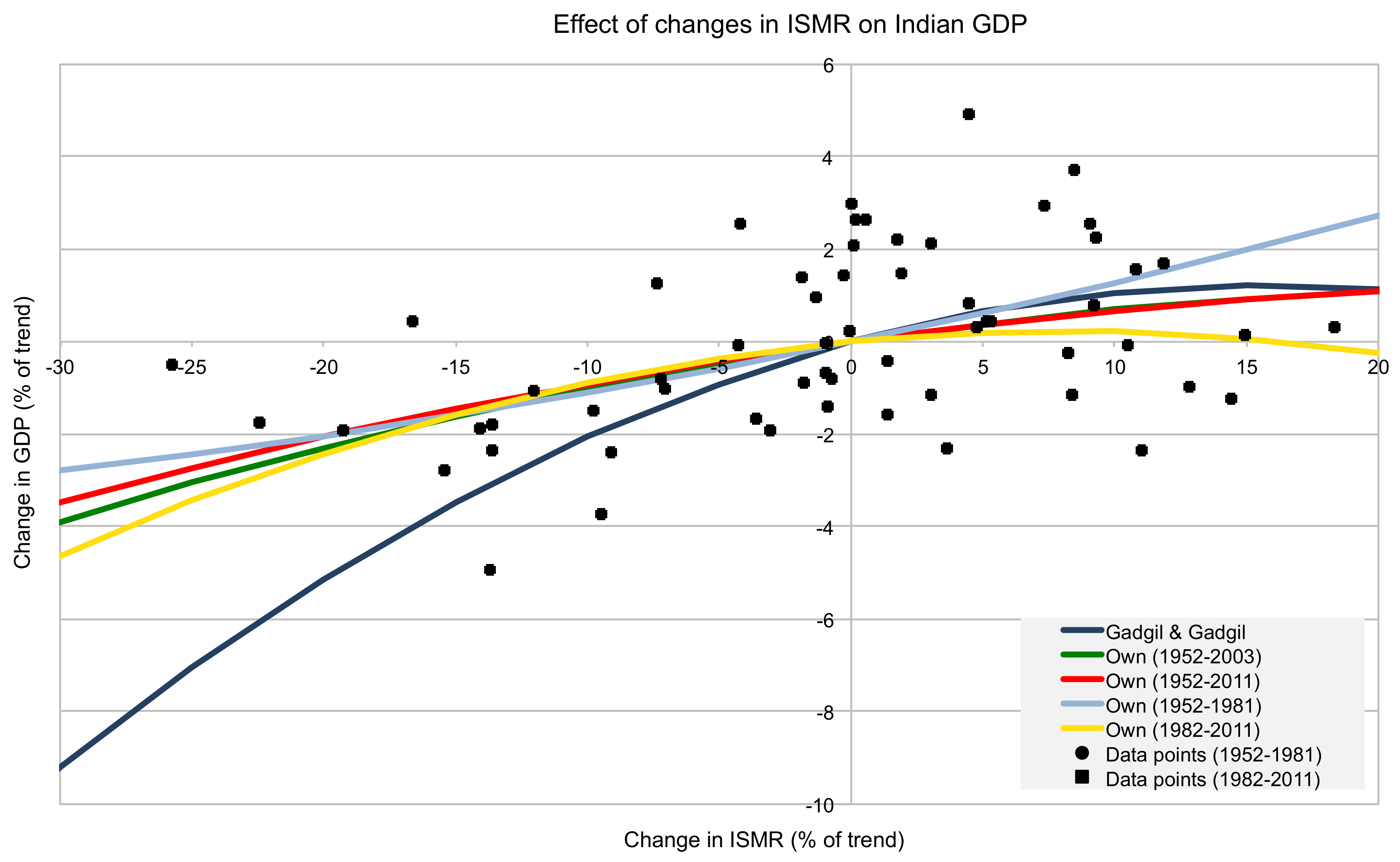
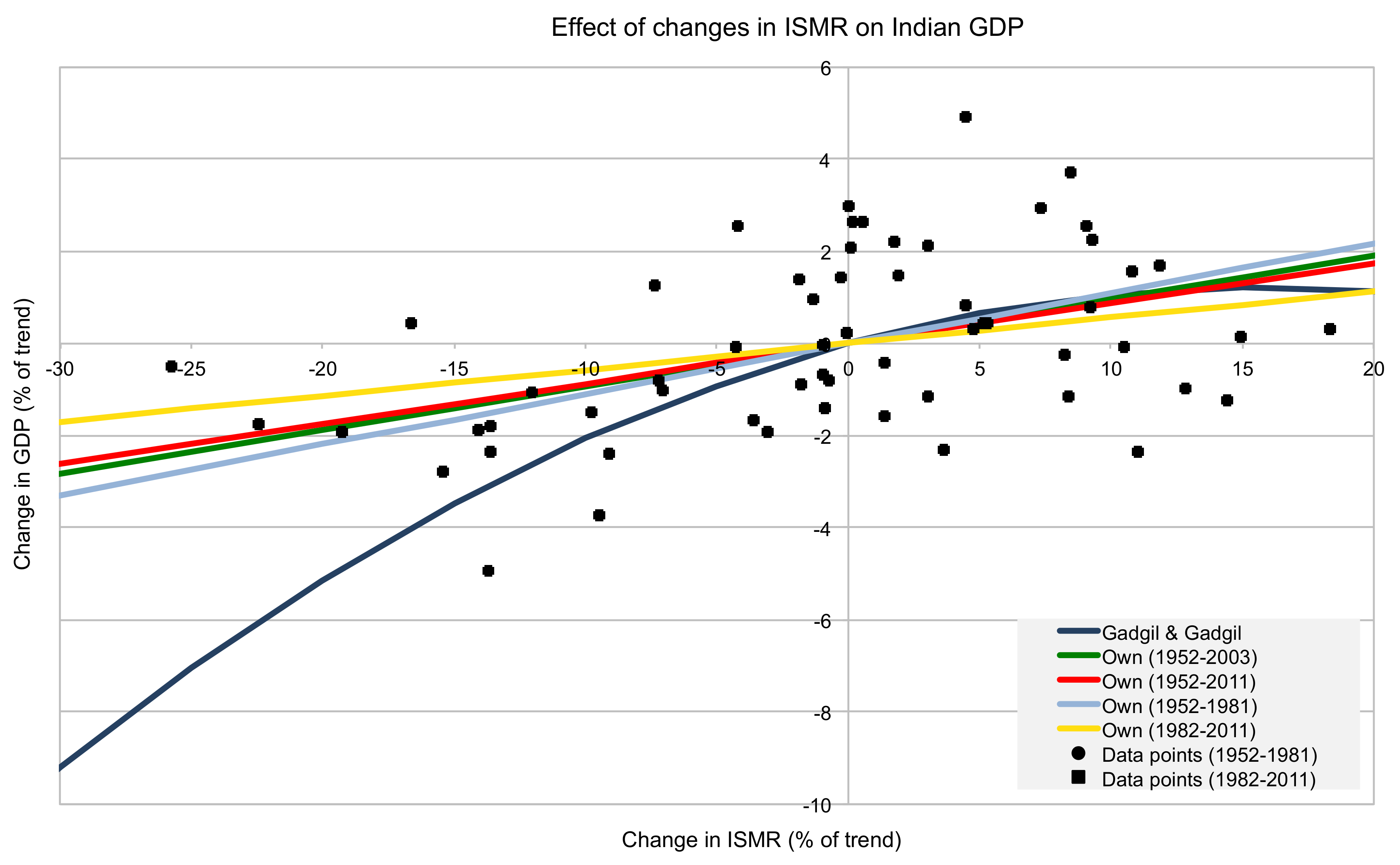
These relationships are found by plotting the yearly deviations of GDP and ISMR from their respective trends (see below). The trends are defined by best-fit curves which remove the shorter-term variability but retain the longer term developments (GDP’s trend is defined as a sextic curve, while ISMR’s trend is defined using an inverted quadratic curve, peaking around 1955). In the first instance, inverted quadratic fit curves are used (Figure 4 and

Table 2. Coefficients for the modelled (quadratic) relationships between ISMR and GDP as described in Figure 4, where a is the coefficient for the quadratic term and b is the coefficient for the linear term. Additionally, the standard error of the deviation of the relevant data points shown and the modelled curve. The standard error calculated for (i) is based on the updated datasets used for the other relationships but using the years and constants as given in Reference [15].

Relationship	a		b		Residual Standard Error
	Value	Standard Error	Value	Standard Error
Gadgil and Gadgil (i)	−0.005	-	0.1565	-	-
1952–2003 (ii)	−0.00152	0.00168	0.0842	0.0284	1.82
1952–2011 (iii)	−0.00122	0.00155	0.0786	0.0255	1.76
1952–1981 (iv)	0.00089	0.00240	0.1191	0.0443	2.007
1982–2011 (v)	−0.00331	0.00220	0.0547	0.0295	1.45

) as used by Gadgil and Gadgil [14]. The quadratic coefficients are found to be statistically insignificant and so the results for linear fits are also presented (Figure 5 and

Table 3. As Table 2 but for a linear fit model of the relationship between ISMR and GDP (i.e., the values for a are 0).

Relationship	b		Residual Standard Error
	Value	Standard Error
Gadgil and Gadgil (i)	-	-	-
1952–2003 (ii)	0.0946	0.0259	1.81
1952–2011 (iii)	0.0863	0.0235	1.75
1952–1981 (iv)	0.1096	0.0354	1.98
1982–2011 (v)	0.0565	0.0301	1.48

). In real-world terms, the inverted quadratic curve makes sense physically as at some point increased rainfall will result in flooding and significant economic costs (see [14] for more details). We present results for both cases here.

In all cases the relationships between GDP and ISMR have lower gradients than the one reported in Gadgil and Gadgil [14] below 0 deviation in ISMR. Further, the relationship derived for the same period (1952–2003) using the updated datasets and methodologies is a closer fit to the other relationships derived here (especially where the ISMR deviation is negative, that is, low rainfall), suggesting a methodological or data divergence between Gadgil and Gadgil and this analysis (A significant difference is the trend lines for GDP and ISMR; Gadgil and Gadgil define it via exponential growth with a different rate either side of 1981, while they use the historical average of ISMR as its trend).

2.3. Relationship between SO₂ Emissions and The Economy

These two primary relationships can be combined to produce relationship between changes in SO₂ emissions and changes in Indian GDP. If total GDP and total SO₂ emissions are known for the relevant catchment areas, then the benefit for a given reduction in SO₂ emissions can be calculated and expressed in a currency per tonne basis.

2.3.1. Total SO₂ Emissions and GDP in Catchment Areas

To determine the overall GDP represented in the catchment area shown in Figure 1, the proportion of the land area within the catchment area is estimated for the relevant countries (or Indian states). The underlying assumption is that the GDP is uniformly distributed over the area of a country or state. The total GDP for the ISMR affected area is calculated by weighting the relevant land area by national GDP (as per the World Bank [20]). The exceptions are for China (Xizang/Tibet) where national statistics (for Xizang/Tibet) are used [21] and India where state GSP (Gross State Product) is taken from nationally compiled statistics [22]. Because the World Bank GDP value for India as a whole differs from the aggregate of the state-wise figures, the total proportion of Indian GDP included in the catchment area is determined by the aggregate of the sum of each state’s GSP multiplied by its included land area. This proportion is then multiplied by the World Bank’s GDP for India to ensure comparability of the Indian figures with other countries. The results of these allocations are shown in

Table A1. Relevant portion of GDP as per the proportion of land area included in the ISMR catchment area based on data from [20] and a visual judgment of the proportion of the country or state included in the area.

Country	State	Land Proportion	Relevant Portion of GDP (US$, 2003)
Bangladesh	-	0.5	30,079,464,594
Bhutan	-	0.33	205,268,616
China	Xizang/Tibet	0.5	1,425,193,000
Indian States	Bihar	1	-
	Chandigarh	1	-
	Chhattisgarh	0.5	-
	Delhi	1	-
	Gujarat	0.8	-
	Himachal Pradesh	1	-
	Jammu & Kashmir	1	-
	Jharkhand	1	-
	Madhya Pradesh	1	-
	Maharashtra	1	-
	Odisha	0.33	-
	Punjab	1	-
	Rajasthan	1	-
	Sikkim	1	-
	Uttar Pradesh	1	-
	Uttarakhand	1	-
	West Bengal	1	-
Indian Total			375,671,613,158
Nepal	-	1	6,330,473,097
Pakistan	-	0.33	27,470,784,361

(Appendix A).

The total SO₂ emissions in the catchment area are calculated by using a gridded SO₂ emissions inventory [23] to determine the total of the emissions originating within the coordinates of the emissions catchment area. By far the largest country (GDP) is India, with 85% of the GDP and an estimated 81% of the SO₂ emissions.

2.3.2. Factor of Reliance on Rainfall

The relationship between ISMR and GDP provided in Gadgil and Gadgil is specific to India, whereas the relationship between SO₂ emissions and ISMR is for areas defined by coordinates, irrespective of national borders. To expand the calculation of the relationship between SO₂ emissions and GDP to all of the included countries, each relevant GDP figure is corrected for the country’s reliance on rainfall relative to India’s. This is done by creating a ‘factor of reliance on rainfall’ for each country, calculated by dividing the factors ‘Agriculture’s contribution to value added—GDP’ [24] by ‘Percentage of arable land equipped for irrigation (%) (3-year average)’ [25] (each indexed to India’s value). The factors are shown in

Table A2. National factors for reliance of GDP on rainfall for 2003 [24,25] calculated from the proportion of each country’s provided by the agricultural sector and the proportion of each country’s arable land with irrigation, all indexed to the respective values for India.

Country	Agriculture’s Contribution to Value Added—GDP	% of Arable Land Equipped for Irrigation (%) (3yr avg)	GDP Reliance on Rainfall
Bangladesh	0.97	1.43	0.68
Bhutan	1.17	0.53	2.23
China	0.57	1.33	0.43
India	1.00	1.00	1.00
Nepal	1.75	1.28	1.37
Pakistan	1.09	1.48	0.74

(Appendix A).

2.3.3. Unit Benefit of South Asian SO₂ Emissions

The change in GDP for a 1% reduction of SO₂ emissions across the catchment area is calculated for each country, assuming a linear relationship between emissions reduction and increased ISMR. Each country’s GDP is adjusted to account for the proportion of the country included in the catchment area, the relative reliance on rainfall and the proportion of GDP from agriculture. This benefit is then divided by the mass (in tonnes) of SO₂ represented by a 1% reduction of the regional emissions (adjusted to include only emissions from months in the monsoon season (see below)). The marginal benefit of SO₂ emissions per tonne (US$/t) is then found by dividing the GDP benefit of a 1% reduction by the pertinent mass of SO₂.

For the secondary analysis of the benefit of only Indian emissions on only the Indian economy, India’s proportion of the total SO₂ emissions within the emissions catchment is calculated using data for individual countries and the catchment area as a whole [23]. Assuming only India would reduce their emissions, the calculation of GDP benefit deriving from any reduction in SO₂ emissions is adjusted by the Indian proportion of emissions and applied to only the relevant portion of Indian GDP (all-India or Agriculture and allied services).

2.3.4. Proportional Impact of All Emissions

Sulphate aerosol has an atmospheric lifetime of a few days (especially in an active monsoon), so only SO₂ emissions during and/or immediately preceding the monsoon season cause any reduced rainfall. For example, Dave et al. [8] observe a lag of 1–5 days between high AOD (aerosol optical depth, that is, high concentration of SO₂ and other aerosols) and suppressed rainfall. For this analysis, the primary assumption is that only SO₂ emissions from May-September, that is, the monsoon season and the preceding month, affect ISMR. The monthly proportion of SO₂ emissions is approximated by the monthly electricity generation (60% of Indian SO₂ emissions [23]) as a proportion of the annual total for 2012–3 [26,27]. The proportions for each group of months are shown in

Table A3. Proportion of Indian annual electricity generation for the respective groups of months on and/or preceding the monsoon season for 2012–13 [26,27].

Year	Months
	JJAS	MJJAS	AMJJAS
2012–3	0.337	0.423	0.502

(Appendix A).

2.3.5. Cost Imposed on Agriculture from Burning Coal

A useful method of contextualising the magnitude of the effect of SO₂ emissions on India’s GDP is to calculate the cost of the activities which result in SO₂ emissions in terms of the negative effect they have on the economy. Around 63% of India’s SO₂ emissions are caused by coal combustion [28], so a cost per tonne of coal burned is a sensible unit of comparison. According to Mittal et al. [29](pp. 4 & 5), the mass of SO₂ emitted is equal to the sulphur content multiplied by 2 (64/32) and Indian coal has a sulphur content of 0.2–0.7%. Thus 9 g of SO₂ are emitted per tonne of coal burned. This is multiplied by the unit benefit ($/t) of SO₂ emissions mitigation to find the level cost per tonne of coal burned.

3. Results

3.1. Unit Benefit of South Asian SO₂ Emissions Mitigation

Table 4. Effect of 1% reduction in regional SO₂ emissions in term of emissions mass, GDP benefit and unit GDP benefit.

Year/Scenario	1% Reduction of South Asian SO2 Emissions
	Mass of Reduction (t)	Benefit (m. US$)	Unit Benefit (US$/t)
2003	31,000	26	830

shows the effect of atmospheric sulphate and the relative benefit of a 1% reduction of South Asian SO₂ emissions, how much SO₂ this 1% reduction represents and the unit benefit resulting from the SO₂ mitigation. (More detail can be found in in Table A3 in Appendix A).

Table 5. County by country breakdown of the proportional benefit of SO₂ emissions mitigation according to relative economy size, reliance on rainfall for agricultural GDP generation and proportion of country included in the ISMR catchment area.

Country	Allocation of Emissions and Benefit
Bangladesh	4.8%
Bhutan	0.1%
China	0.1%
India	88.2%
Nepal	2.0%
Pakistan	4.7%

shows the breakdown of the unit benefit of SO₂ emissions mitigation benefit according to the proportional land areas of each country in the ISMR and SO₂ emissions catchment areas (assuming spatial uniformity of GDP across the land area). Additionally, each country’s economic reliance on rainfall relative to India’s is accounted for.

India dominates the calculation, with 88% of the effect coming from their emissions and actions. This is to be expected as the intention of the catchment areas as defined by Guo et al. [13] is to analyse India. Further, India is the largest economy and SO₂ emitter in the catchment areas (Table A1, Appendix A). On this basis the further results presented here concentrate on India only.

3.2. Unit Benefit for India Only

As shown in

Table 6. Unit benefit of SO₂ emissions reduction for the whole Indian economy and the subset of Agriculture and allied services based on the quadratic relationship between ISMR and GDP, for the years 1952–2011 and 1982–2011 and for three different scenarios of the period in which SO₂ emissions affect ISMR: June–September (JJAS), May–September (MJJAS) and April–September (AMJJAS).

Year/Scenario	Unit Benefit of SO2 Reduction (US$/t)
	JJAS	MJJAS	AMJJAS
Agriculture and allied services GDP (1952–2011)	158	126	106
Agriculture and allied services GDP (1952–1981)	138	110	93
Agriculture and allied services GDP (1982–2011)	209	166	140
All India GDP (1952–2011)	501	400	337
All India GDP (1952–1981)	443	354	298
All India GDP (1982–2011)	643	513	432

for the updated, India-only scenarios, the benefit of marginal SO₂ mitigation ranges is substantial. Taking the case where emissions from May-September are effective and there is a quadratic dependence of GDP on ISMR, each tonne of SO₂ not emitted would have been accompanied by an increase to the agricultural and allied services sector of US$110–166 (taking the values for the 1952–1981 and 1982–2011 periods) or to the wider economy of US$354–513 (same periods). It bears repeating that these figures exclude the negative effects of SO₂ on crop and human health. Notably, the benefit is greater in the latter years (1982–2011) and much greater for the whole economy compared to the agriculture and allied sector in isolation, implying that the effect of ISMR extends well beyond the boundaries of the ‘Agriculture and allied services’ sector.

Table 6 also shows the benefit of SO₂ emissions mitigation assuming emissions from other periods affect ISMR: June–September (JJAS) and April–September (AMJJAS). Monthly electricity generation is used as a proxy for SO₂ emissions, with the proportion of the yearly total generation in each period representing each period’s proportion of SO₂ emissions (Table A1, Appendix A).

As expected, the unit benefit of SO₂ mitigation on GDP changes significantly—approximately by 1/12th per month as electricity generation is fairly steady throughout the year—as the duration of effective emissions is changed. If SO₂ emissions from only the monsoon season (June–September) are considered, the unit benefit of SO₂ emissions mitigation rises to up to US$643/t.

Table 7. As Table 6 based on the linear relationship between ISMR and GDP. The numbers in parentheses are the one sigma uncertainty derived using the standard errors in Table 3.

Year/Scenario	Unit Benefit of SO2 Reduction (US$/t)
	JJAS	MJJAS	AMJJAS
Agriculture and allied services GDP (1952–2011)	134 (21)	107 (17)	90 (14)
Agriculture and allied services GDP (1952–1981)	156 (30)	124 (24)	105 (20)
Agriculture and allied services GDP (1982–2011)	104 (29)	83 (23)	70 (20)
All India GDP (1952–2011)	400 (109)	319 (87)	269 (73)
All India GDP (1952–1981)	495 (160)	395 (128)	333 (108)
All India GDP (1982–2011)	266 (142)	212 (113)	179 (95)

shows the results based on the linear fits as well as the 1 sigma uncertainties found by propagating the standard errors calculated using the linear fit presented in Table 3. For the period 1952–2011, the results for the agriculture and allied services GDP and for the all-India GDP are similar, though slightly smaller, than the results derived using a quadratic relationship. However the unit benefit calculated for 1982–2011 is smaller than that for 1952–1981 indicating a possible increase in resilience of the Indian economy to interannual variability in monsoon rainfall. It is important to note that this estimate of the uncertainty is an underestimate as while it includes the errors associated with the relationship between ISMR and GDP, it does not include any uncertainty associated with the relationship between SO₂ emissions and rainfall from Guo et al. [3], presented in Table 1.

Cost of Burning Coal

Another manner of describing the unit benefit of SO₂ emissions is that of the benefit of not burning a tonne of coal.

Table 8. Cost on economy of the SO₂ emissions from burning one tonne of Indian coal according to the total cost of the emissions and the SO₂ emissions of coal burning for both a quadratic and a linear relationship between ISMR and GDP, with uncertainties presented as per Table 6.

Year/Scenario	Cost on Agriculture from Burning Coal during MJJAS Months (US$/t)
	Quadratic Fit	Linear Fit
Agriculture and allied services GDP (1952–2011)	1.14	0.97 (0.15)
Agriculture and allied services GDP (1952–1981)	0.99	1.12 (0.22)
Agriculture and allied services GDP (1982–2011)	1.5	0.74 (0.21)
All India GDP (1952–2011)	3.6	2.87 (0.78)
All India GDP (1952–1981)	3.18	3.55 (1.15)
All India GDP (1982–2011)	4.61	1.91 (1.02)

shows the results of this calculation in terms of the cost to agriculture and allied services or the whole economy, of the resulting SO₂ emissions. For reference, coal prices are around US$40–100 [30].

Again under the baseline assumption that only emissions from May-September affect ISMR, the economic effect of not burning 1 tonne of Indian coal is from US$1.0 to $4.6 (INR64 to 297) for the quadratic fit and slightly less (US$0.74 to US$3.6) for the linear fit.

A similar analysis was performed for another significant contributor to Indian SO₂ emissions: transport fuels. The results were insignificant on an agricultural cost per litre basis due to the much lower sulphur content of Indian diesel fuel (50–300 ppm) compared to coal (≈450,000 ppm).

4. Discussion

The estimated costs described above can be viewed either as hidden costs or as potential benefits which would result from any actions taken to reduce sulphur emissions in the region, for example, by reducing coal burning, whatever the motivation for the action. India’s overall energy consumption is growing by 4.2% per annum which is faster than all other major economies [31]. Coal is the biggest component of the energy supply mix, though renewables are increasing rapidly as a result of India’s commitments under the 2015 Paris Agreement. Renewables are forecast to be the second largest energy source by 2020. Overall though, India’s energy mix is evolving slowly and coal is forecast to only fall from 57% of total generation in 2016 to 50% in 2040 [31]. It is worth noting here that if India’s growing energy needs had been met only by coal burning, then the indirect costs of reduced rainfall on India would have been greater. These ‘savings’ should be included in assessments of the past and future costs of the transition from coal to renewable energy sources.

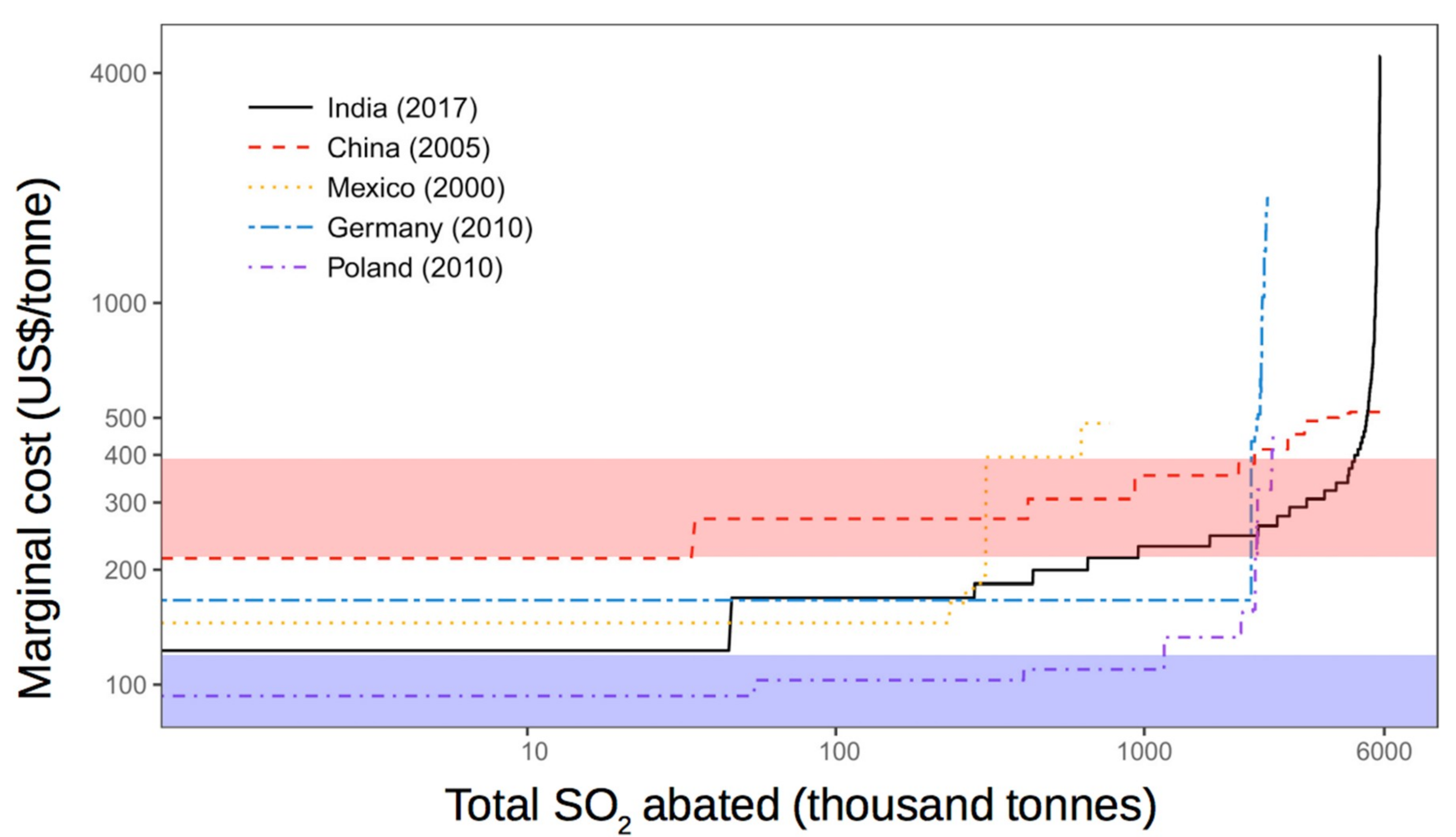
Whatever the broader context of coal use in Indian economy (and India is selected for further analysis here because of its dominance as an emitter and from the effect on its agricultural sector), the marginal gains resulting from other SO₂ emissions mitigation measures can be assessed. The information presented above is put into context by Figure 6, (adapted from [32]) which shows the marginal cost of abatement for SO₂ from coal-fired power plants in India, China, Mexico, Germany and Poland. The coloured bands represent the estimated marginal costs on the agricultural and allied services (blue: 83–124 US$/tonne) and on the overall economy (red: 212–396 US$/tonne) based on the linear fits. If the true numbers lie at the upper end of the range for the whole economy, approximately 5 million tonnes of SO₂ emissions (~50 % of India’s 2012 emissions) could be mitigated at no net cost or a net benefit. The large range and the uncertainties associated with the underlying estimates (Table 7) show the need for further analyses based on this or a similar methodology.

Further context is provided by Cropper et al. [33], who analyse the net benefit or cost on human mortality of air pollution controls (i.e., flue-gas desulfurisation or FGD) on a theoretical 500MW coal-fired power plant in eight locations across India. At each location they consider four scenarios of Value per Statistical Life (VSL) (US$84,000–$256,000) and discount value (3%, 8% and 12%). From their results, using the given assumptions on power plant annual emissions and operational lifetime, we derive the net benefit of SO₂ abatement ranges from US$ −234 (i.e., a net cost) per tonne of SO₂ to $7020 (a net benefit) with an average of US$1,071. As such, the benefits of SO₂ emissions mitigation/abatement from EIR add around 20–37% to the benefits from human mortality. Furthermore, where SO₂ mitigation is a net cost (US$ −234/t) considering human mortality, the addition of the most conservative benefit from EIR ($212/t) is almost sufficient to make the mitigation actions cost neutral.

The unit benefit of SO₂ emissions mitigation is lower in 1982–2011 compared to in 1952–2003, although the magnitude by which this is the case is unexpected. This could be down to differences in the methodology, however or to an increased resilience in India’s infrastructure.

Another somewhat surprising result is the difference in benefit found between the agricultural and allied sector and the whole economy. The original assumption underlying our analysis of the relationship between ISMR and GDP was that this is underpinned by the EIR through crop yields. The result presented here suggests the EIR is more wide-reaching, with greater benefits outside the defined agriculture and allied services sector than within it. This could be down to the fact that the boundary for the agricultural and allied sector as provided in Reference [17] is set so that it does not capture sufficient effects of ISMR for this analysis, for example, the flow-on effects for the whole economy are very large in comparison to the direct effects on the agricultural sector. Alternatively, other effects of ISMR occurring outside the agricultural sector (i.e., not considered here) could be important. Regardless, this analysis is ultimately not concerned with how the EIR is manifest, rather how large it is, so All-India GDP is the more appropriate object of study in this case.

4.1. Policy Implications

On a basic level, this analysis shows that there are economic benefits to reducing SO₂ emissions in the crucial monsoon months. As such, it would be economically as well as environmentally sensible to implement policies that encourage or enforce this reduction. The benefits result from and are experienced by the same region (South Asia), particularly India, where the emissions take place. As such, any policy action taken by India would have a direct effect on (primarily) India, avoiding a tragedy of the commons style scenario, as seen in climate change action, whereby there is only an indirect link between actions (and their costs) and the benefits.

This analysis presents evidence that the actions of one sector (SO₂ emissions, primarily from electricity generation) have a direct detrimental effect on the economy. Accordingly, assuming EIR is indeed primarily on agriculture (and flow-on effects), a redistributive policy could be implemented, whereby a charge is applied to SO₂ emissions during the crucial monsoon months and redistributed to farmers or other affected parties to compensate them for the lost income caused by the EIR as a result of the SO₂ emissions. This analysis shows that such a charge would be a significant fraction of the current cost of coal and it would be higher if other factors such as human health effects are included. Alternatively, an SO₂ emissions trading scheme could be implemented, with higher emissions costs in the crucial months.

If applied to actual emissions (rather than potentially emitting activities), such a charge would also have the positive effect of providing an economic disincentive on SO₂ emissions and thus would provide an economic incentive on the fitment of abatement technologies or non-emitting alternatives (e.g., renewable electricity generation) which would likely have a positive effect beyond the agricultural sector in India and South Asia. In extreme cases, some SO₂ emitting activities might simply cease (in the relevant periods).

4.2. Uncertainties Identified

Developing an appropriate policy response would require improved analyses along the lines of the methodology developed here. The following uncertainties have been identified related to this analysis in addition (except where noted) to the statistical uncertainties as presented previously.

• The relationship between ISMR and GDP is slightly better modelled as linear compared to an inverted quadratic relationship. The statistical uncertainties for the linear relationship have been identified and presented in Table 7 and Table 8. Nonetheless a linear relationship predicts increased economic output for increased rainfall ad infinitum, which must deviate from reality at some point as at some point increased rainfall will cause flooding and decreased economic output. This phenomenon is plausibly represented by using an inverted quadratic relationship but the true relationship is unknown.
• The distribution of GDP generation is assumed to be uniformly distributed spatially, whereas this is unlikely to be the case, with it likely to be concentrated in certain regions.
• The relationship between SO₂ and ISMR is assumed to be linear. The baseline paper’s [13] scenarios only consider full emissions or full mitigation of SO₂, while this analysis assumes that for example, a 50% reduction would be associated with a 50% effect on ISMR. This may not be the case.
• Indian SO₂ emissions are assumed to follow the seasonal pattern of electricity generation. While this is the dominant source of SO₂ in India, the distribution may show greater or lesser seasonality than that of electricity generation.
• The effects of the ISMR on the wider economy (i.e., beyond ‘agriculture and allied services’) are uncertain and it is important to understand them better qualitatively and quantitatively.
• The EIR is not fixed. It is influenced by the level of (irrigation) technology and crop choice and presumably on the quality of the weather forecasts and the resilience of the broader Indian infrastructure. The representation of aerosols in climate models is relatively simple and there are large uncertainties in the impact of aerosol loading on precipitation. Improved models and a range of specially designed scenarios could be used to investigate this further. These could include different choices of areas of emissions and impact than in Figure 1. Further investigation of the relative importance of local and remote emissions is required.

5. Conclusions

We present a methodology to estimate the possible effect on the Indian economy of changes in SO₂ emissions. The preliminary analysis presented in this paper highlights the significant link between SO₂ emissions and reduced monsoon rainfall and thus reduced GDP, presumably primarily driven by crop yields. The situation is relatively simple from an economic and political standpoint: SO₂ emissions (dominated by the electricity sector) in India have a short term but significant, negative impact on rainfall, India’s agricultural sector and the nation’s GDP. As such, a case can be made for action to mitigate SO₂ emissions, particularly in the crucial (pre-) monsoon period, as this would have a significant positive effect on a crucial and large part of India’s economy. The effects would be visible almost instantly. There have already been large and, likely, unaccounted for benefits resulting from the growth in renewable energies in India. These indirect benefits should be included when assessing the cost of this transition, as should any other indirect benefits such as health gains through improved air quality. A political option which could be effective in further accelerating this transition from coal-burning would be to have a redistributive charge on SO₂ emitting activities (during the crucial period). The proceeds could be used to compensate farmers (or other groups) for lost income and would provide an economic disincentive on SO₂ emissions which would have positive effects on global SO₂ levels and local human and crop health.

Further work involving improved process understanding, focused model runs and more granulated economic data, as highlighted in Section 4.2, would improve the methodology and reduce uncertainties associated with the preliminary results presented here as well as offer the opportunity to address more focused policy questions.

References

- Turner, A.G.; Annamalai, H. Climate change and the South Asian summer monsoon. Nat. Clim. Change 2012, 2, 587–595. [Google Scholar] [CrossRef]
- Patil, N.; Venkataraman, C.; Muduchuru, K.; Ghosh, S.; Mondal, A. Disentangling sea-surface temperature and anthropogenic aerosol influences on recent trends in South Asian monsoon rainfall. Clim. Dyn. 2018. [Google Scholar] [CrossRef]
- Guo, L.; Turner, A.G.; Highwood, E.J. Impacts of 20th century aerosol emissions on the South Asian monsoon in the CMIP5 models. Atmospheric Chem. Phys. 2015, 15, 6367–6378. [Google Scholar] [CrossRef]
- Bollasina, M.A.; Ming, Y.; Ramaswamy, V. Anthropogenic Aerosols and the Weakening of the South Asian Summer Monsoon. Science 2011, 334, 502–505. [Google Scholar] [CrossRef] [PubMed]
- Ganguly, D.; Rasch, P.J.; Wang, H.; Yoon, J.-H. Climate response of the South Asian monsoon system to anthropogenic aerosols: Climate Effects of Anthropogenic Aerosol. J. Geophys. Res. Atmospheres 2012, 117, n/a. [Google Scholar] [CrossRef]
- Ganguly, D.; Rasch, P.J.; Wang, H.; Yoon, J. Fast and slow responses of the South Asian monsoon system to anthropogenic aerosols: Fast and Slow Response to Aerosols. Geophys. Res. Lett. 2012, 39. [Google Scholar] [CrossRef]
- Patil, N.; Dave, P.; Venkataraman, C. Contrasting influences of aerosols on cloud properties during deficient and abundant monsoon years. Sci. Rep. 2017, 7, 44996. [Google Scholar] [CrossRef] [PubMed]
- Dave, P.; Bhushan, M.; Venkataraman, C. Aerosols cause intraseasonal short-term suppression of Indian monsoon rainfall. Sci. Rep. 2017, 7, 17347. [Google Scholar] [CrossRef] [PubMed]
- Bollasina, M.A.; Ming, Y.; Ramaswamy, V.; Schwarzkopf, M.D.; Naik, V. Contribution of local and remote anthropogenic aerosols to the twentieth century weakening of the South Asian Monsoon: Aerosols and South Asian Monsoon. Geophys. Res. Lett. 2014, 41, 680–687. [Google Scholar] [CrossRef]
- Vinoj, V.; Rasch, P.J.; Wang, H.; Yoon, J.-H.; Ma, P.-L.; Landu, K.; Singh, B. Short-term modulation of Indian summer monsoon rainfall by West Asian dust. Nat. Geosci. 2014, 7, 308–313. [Google Scholar] [CrossRef]
- Prasanna, V. Impact of monsoon rainfall on the total foodgrain yield over India. J. Earth Syst. Sci. 2014, 123, 1129–1145. [Google Scholar] [CrossRef]
- CMIP–Overview. Available online: https://cmip.llnl.gov/index.html (accessed on 6 February 2019).
- Guo, L.; Turner, A.G.; Highwood, E.J. Local and remote impacts of aerosol species on Indian summer monsoon rainfall in a GCM. J. Clim. 2016, 29, 6937–6955. [Google Scholar] [CrossRef]
- Google Earth. Available online: https://www.google.com/earth/ (accessed on 19 November 2018).
- Gadgil, Su.; Gadgil, Si. The Indian Monsoon, GDP and agriculture. Econ. Polit. Wkly. 2006, 41, 4887–4895. [Google Scholar]
- Somasundar, K. All India Area Weighted Monthly, Seasonal And Annual Rainfall. Available online: https://data.gov.in/catalog/all-india-area-weighted-monthly-seasonal-and-annual-rainfall-mm (accessed on 10 October 2018).
- Ashok, A. Sonkusare GDP of India and major Sectors of Economy, Share of each sector to GDP and Growth rate of GDP and other sectors of economy 1951-52 onward. Available online: https://data.gov.in/resources/gdp-india-and-major-sectors-economy-share-each-sector-gdp-and-growth-rate-gdp-and-other (accessed on 10 October 2018).
- North Eastern Council, Government of India Agriculture and Allied. Available online: http://necouncil.gov.in/nec-project-sector/agriculture-and-allied (accessed on 21 December 2018).
- (Indian) Ministry of Statistics and Program Implementation Statement 30: Domestic Product from Agriculture & Allied Activities (at Current Prices). Available online: http://mospi.nic.in/sites/default/files/reports_and_publication/statistical_publication/National_Accounts/S30.pdf (accessed on 21 December 2018).
- The World Bank GDP (current US$)|Data. Available online: https://data.worldbank.org/indicator/NY.GDP.MKTP.CD (accessed on 25 June 2018).
- National Bureau of Statistics of China National Data-Annual by province (GDP). Available online: http://data.stats.gov.cn/english/easyquery.htm?cn=E0103 (accessed on 26 June 2018).
- (Indian) Ministry of Statistics and Program Implementation State Domestic Product and other aggregates, 2004-05 series. Available online: http://mospi.nic.in/data (accessed on 4 May 2018).
- Crippa, M.; Guizzardi, D.; Muntean, M.; Schaaf, E.; Dentener, F.; van Aardenne, J.A.; Monni, S.; Doering, U.; Olivier, J.G.J.; Pagliari, V.; Janssens-Maenhout, G. Gridded Emissions of Air Pollutants for the period 1970-2012 within EDGAR v4.3.2. Earth Syst. Sci. Data 2018, 1–40. [Google Scholar] [CrossRef]
- The World Bank Agriculture, value added (% of GDP) | Data. Available online: https://data.worldbank.org/indicator/NV.AGR.TOTL.ZS (accessed on 4 May 2018).
- United Nations Food and Agriculture Organization Suite of Food Security Indicators. Available online: http://www.fao.org/faostat/en/#data/FS (accessed on 4 May 2018).
- Central Electricity Authority; Grid Operation & Distribution Wing Load Generation Balance Report (LGBR) for the year 2008-2009. Available online: http://cea.nic.in/reports/annual/lgbr/lgbr-2008.pdf (accessed on 26 June 2018).
- Central Electricity Authority Load Generation Balance Report 2013-14. Available online: http://cea.nic.in/reports/annual/lgbr/lgbr-2013.pdf (accessed on 26 June 2018).
- Smith, S.J.; Van Aardenne, J.; Klimont, Z.; Andres, R. J.; Volke, A.; Delgado Arias, S. Anthropogenic Sulfur Dioxide Emissions, 1850-2005: National and Regional Data Set by Source Category, Version 2.86; NASA Socioeconomic Data and Applications Center (SEDAC): Palisades, NY, USA, 2011. [Google Scholar]
- Mittal, M.L.; Sharma, C.; Singh, R. Estimates of emissions from coal fired thermal power plants in India. In Proceedings of the 2012 International Emission Inventory Conference, Tampa, Florida, USA; 2012; pp. 13–16. [Google Scholar]
- IndexMundi Commodity Prices. Available online: https://www.indexmundi.com/commodities/ (accessed on 28 June 2018).
- BP, p.l.c. BP Energy Outlook Country and regional insights – India. Available online: https://www.bp.com/content/dam/bp/en/corporate/pdf/energy-economics/energy-outlook/bp-energy-outlook-2018-country-insight-india.pdf (accessed on 12 November 2018).
- Sugathan, A.; Bhangale, R.; Kansal, V.; Hulke, U. How can Indian power plants cost-effectively meet the new sulfur emission standards? Policy evaluation using marginal abatement cost-curves. Energy Policy 2018, 121, 124–137. [Google Scholar] [CrossRef]
- Cropper, M.L.; Guttikunda, S.; Jawahar, P.; Lazri, Z.; Malik, K.; Song, X.-P.; Yao, X. Applying Benefit-Cost Analysis to Air Pollution Control in the Indian Power Sector. J. Benefit-Cost Anal. 2018, 1–21. [Google Scholar] [CrossRef]
Figure 1.
Graphic of the catchment areas used by Guo et al. for SO2 emissions and ISMR change (coordinates from [13] (pp. 6943, 6952), visualised in Reference [14]).
Figure 2.
Relationship between ISMR and Indian GDP (redrawn from Gadgil and Gadgil [14]).
Figure 3.
Relationship between ISMR and Indian FGP. The blue line is redrawn from Gadgil and Gadgil [15]. The additional data points are from Prasanna [11], de-indexed using the average total FGP for the years 1966–2007 and from government statistics [16].
Figure 4.
Graph of relationships between ISMR and All-India GDP for five scenarios: (i) the relationship from Gadgil and Gadgil [2006] for data from 1951–2003 (blue); and three (quadratic) relationships we derive using the datasets and methodology described here (ii) for the equivalent period to Gadgil and Gadgil (1951–2003) (green) (iii) using data for 1951–2011 (red); (iv) using the subset of data for 1952–1981 (light blue); and (v) using the subset of data for 1982–2011 (yellow). Annual values are shown for individual years: circles for 1952–1981, squares for 1982–2011—derived from [16,17]).
Figure 5.
As Figure 4 but displaying the linear fit curves (with Gadgil and Gadgil’s quadratic curve for reference).
Figure 6.
Marginal Cost Curve for SO2 abatement from coal-fired power plants in India (solid black curve) and various other countries [32]. The coloured bands represent the estimated marginal cost estimates on the agricultural and allied services (blue: 83–124 US$/tonne) and on the overall economy (red: 212–396 US$/tonne) for the May–September season taken from the linear fits presented in Table 7. The ranges shown are for the central estimates and do not include their uncertainties which are given in Table 7.