Exploring Changes in Land Surface Temperature Possibly Associated with Earthquake: Case of the April 2015 Nepal Mw 7.9 Earthquake

 , ,
, ,
Abstract
:1. Introduction
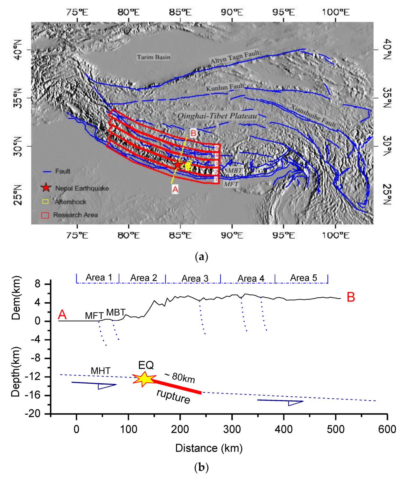
2. The Geological Background and Research Areas
2.1. Geological Background of Southern Margin of the Qinghai-Tibet Plateau
2.2. Areas of Research
3. Data and Methods
3.1. Data
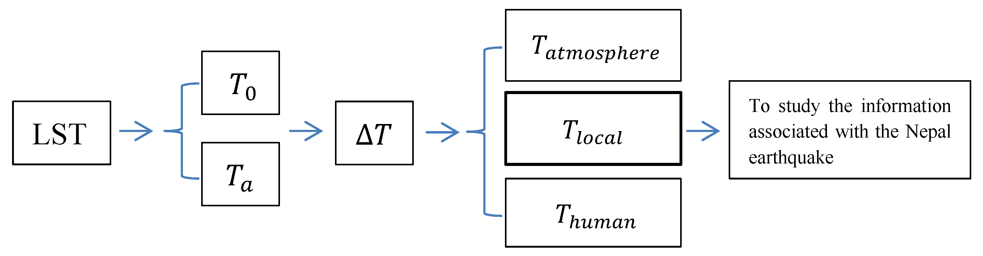
3.2. Methods
3.3. Procedure of Data Processing
4. Results
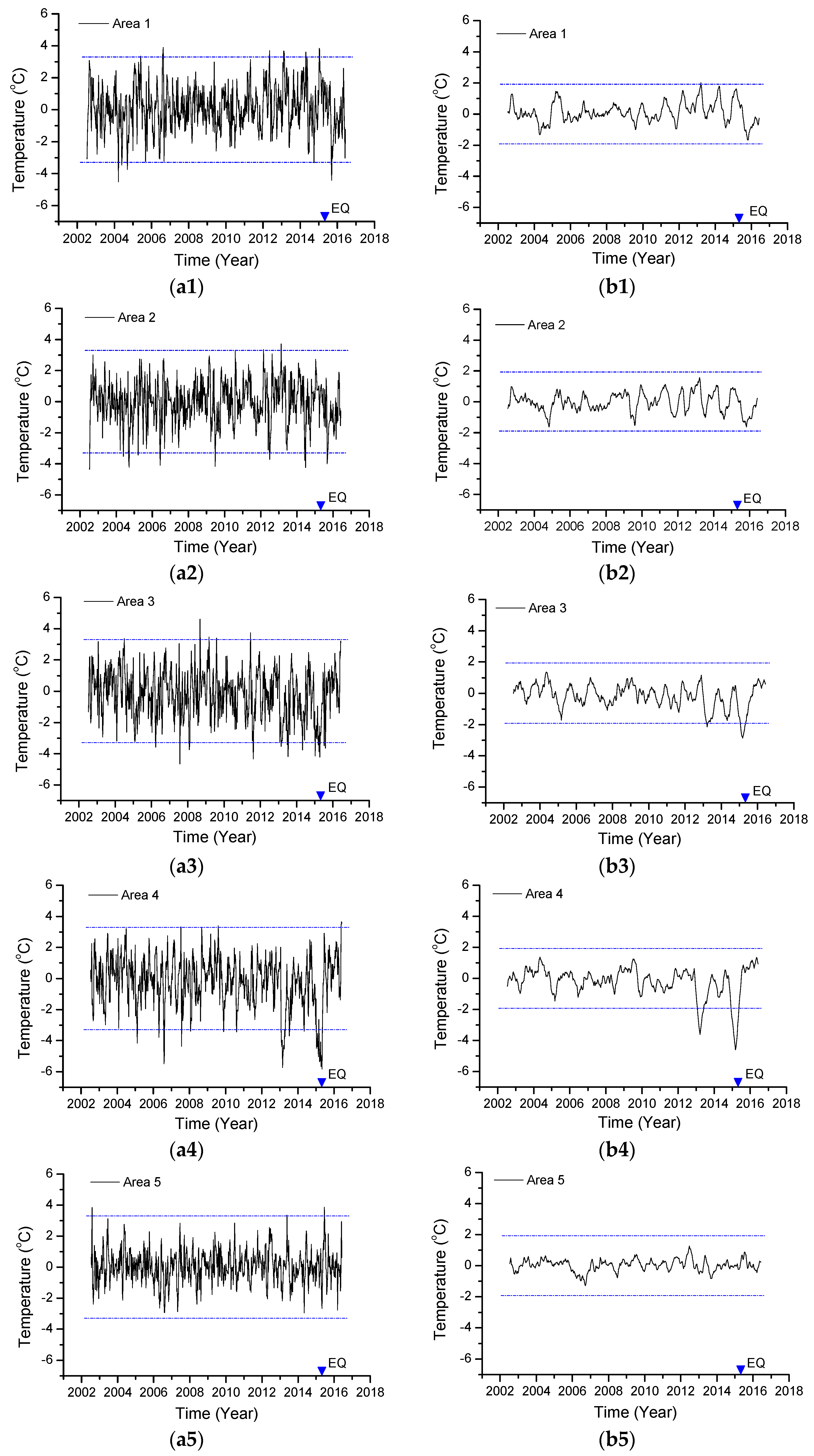
4.1. Temporal Process
4.2. Spatial Distribution
5. Discussion
5.1. Comparison of Two Cooling Events before the Earthquake
5.2. Comparison of Data from Different Satellites
5.3. Physical Mechanism
5.4. Implication of the Coseismic Temperature Response
6. Conclusions
Author Contributions
Funding
Acknowledgments
Conflicts of Interest
Appendix A. One-Dimensional Wavelet Analysis
Appendix B. Two-Dimensional (2D) Wavelet Analysis
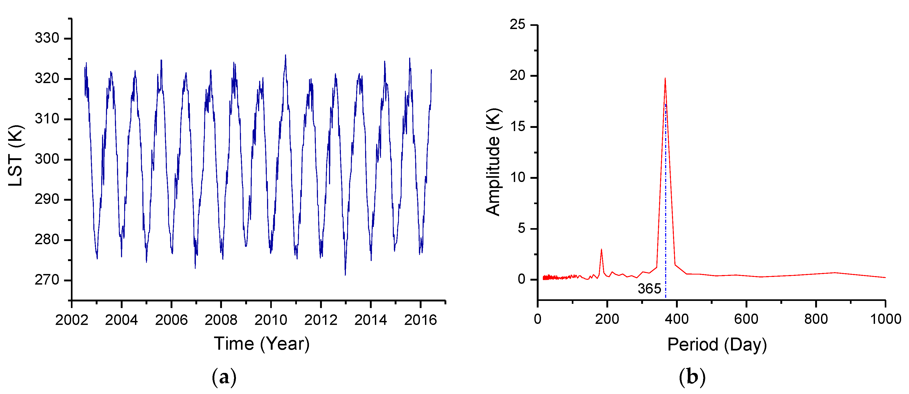
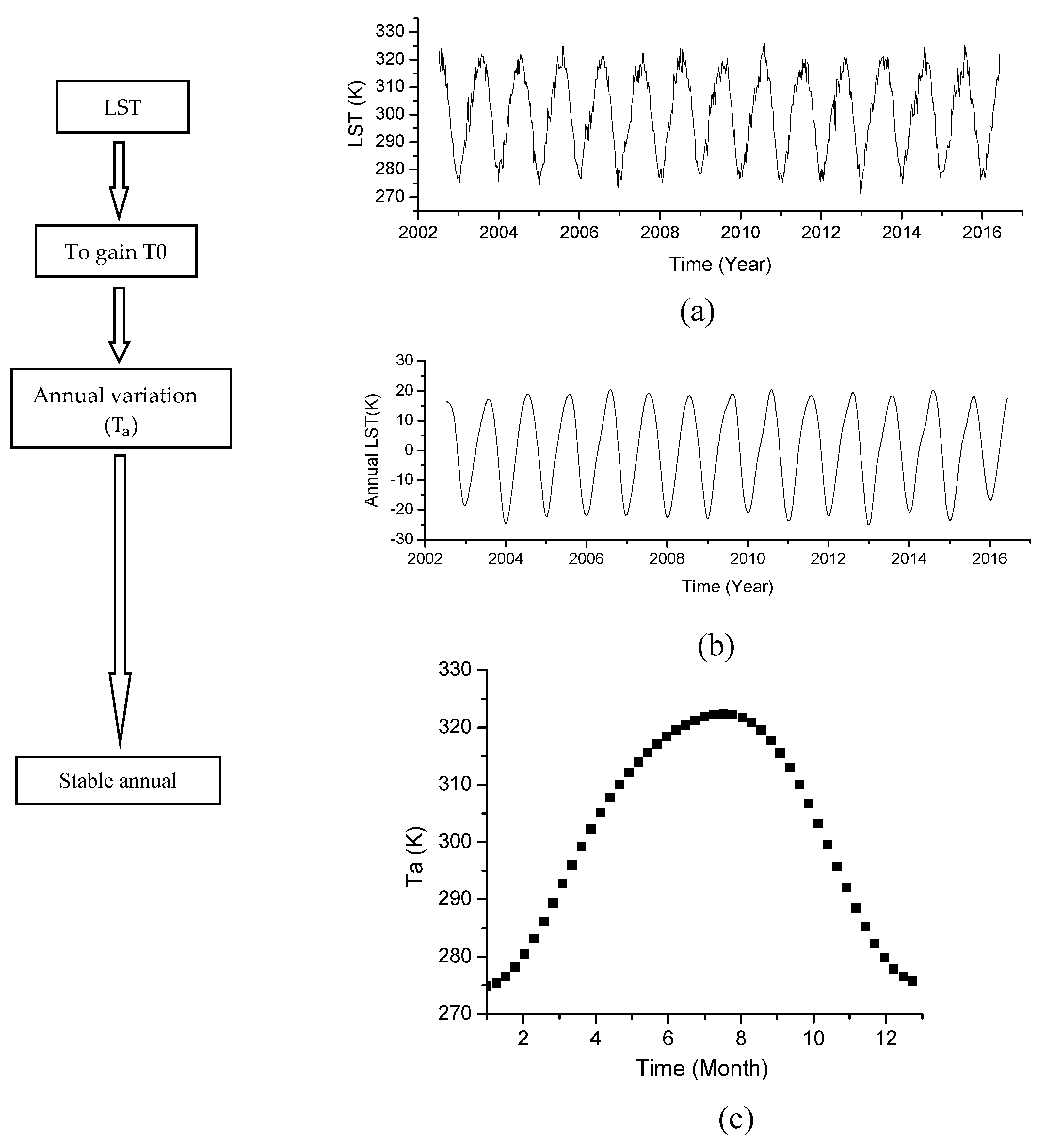
Appendix C. The Stable Annual Variation () in Land Surface Temperature (LST)

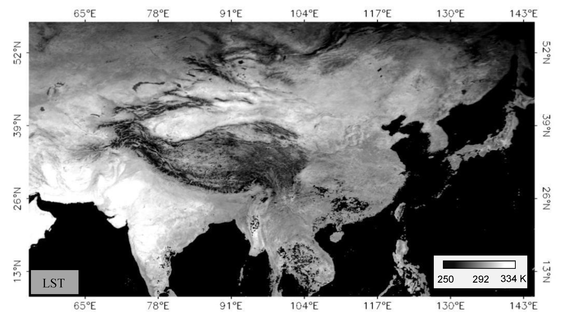
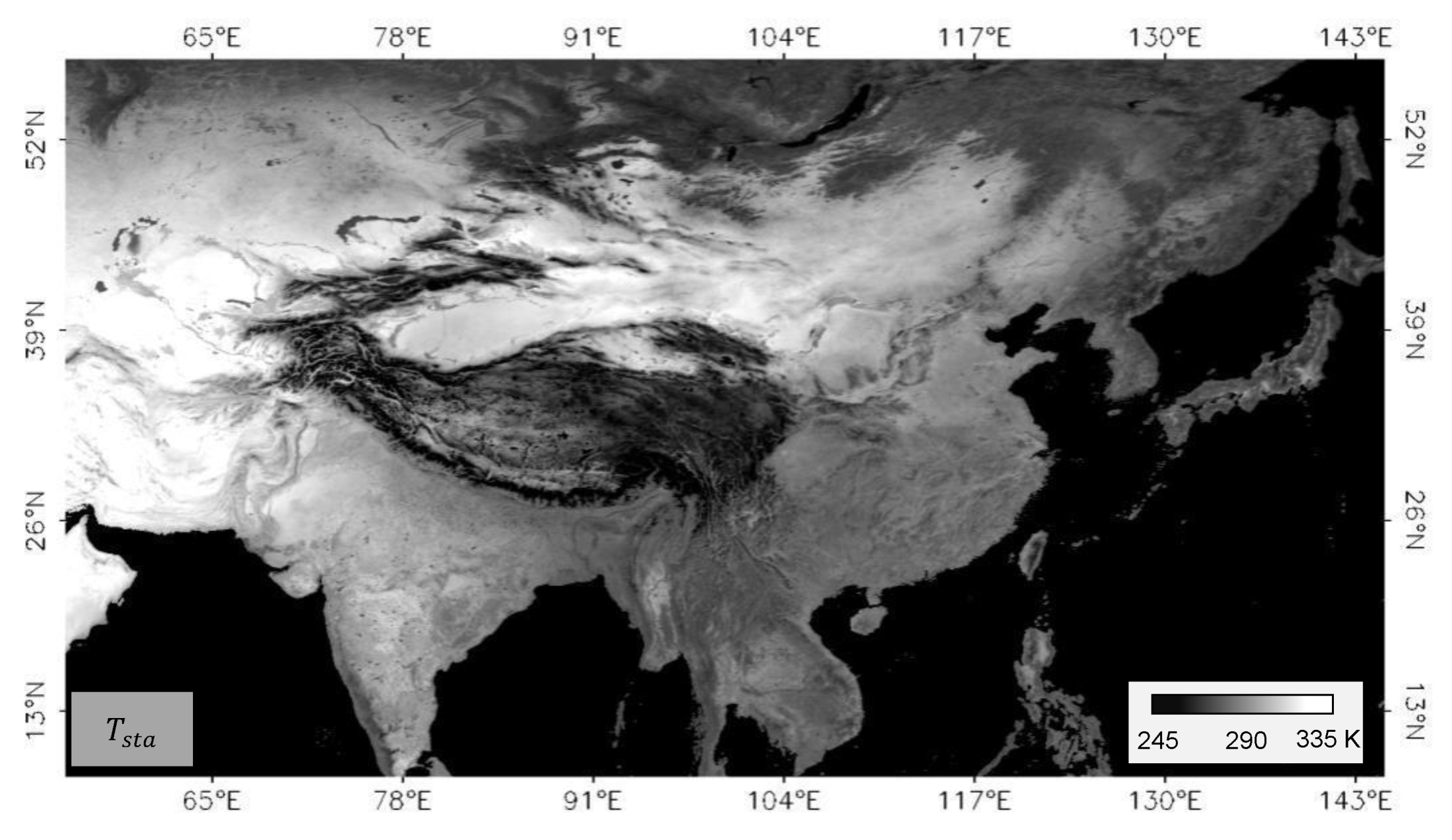
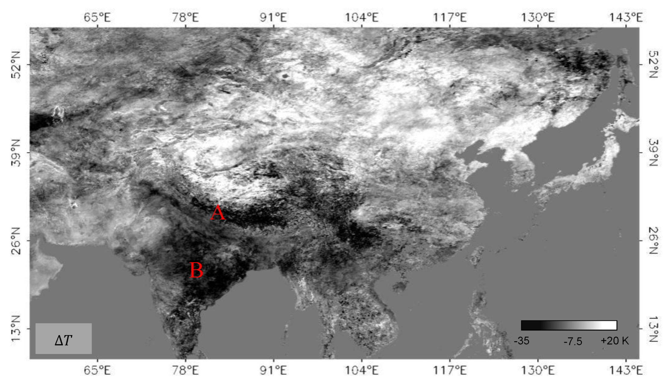
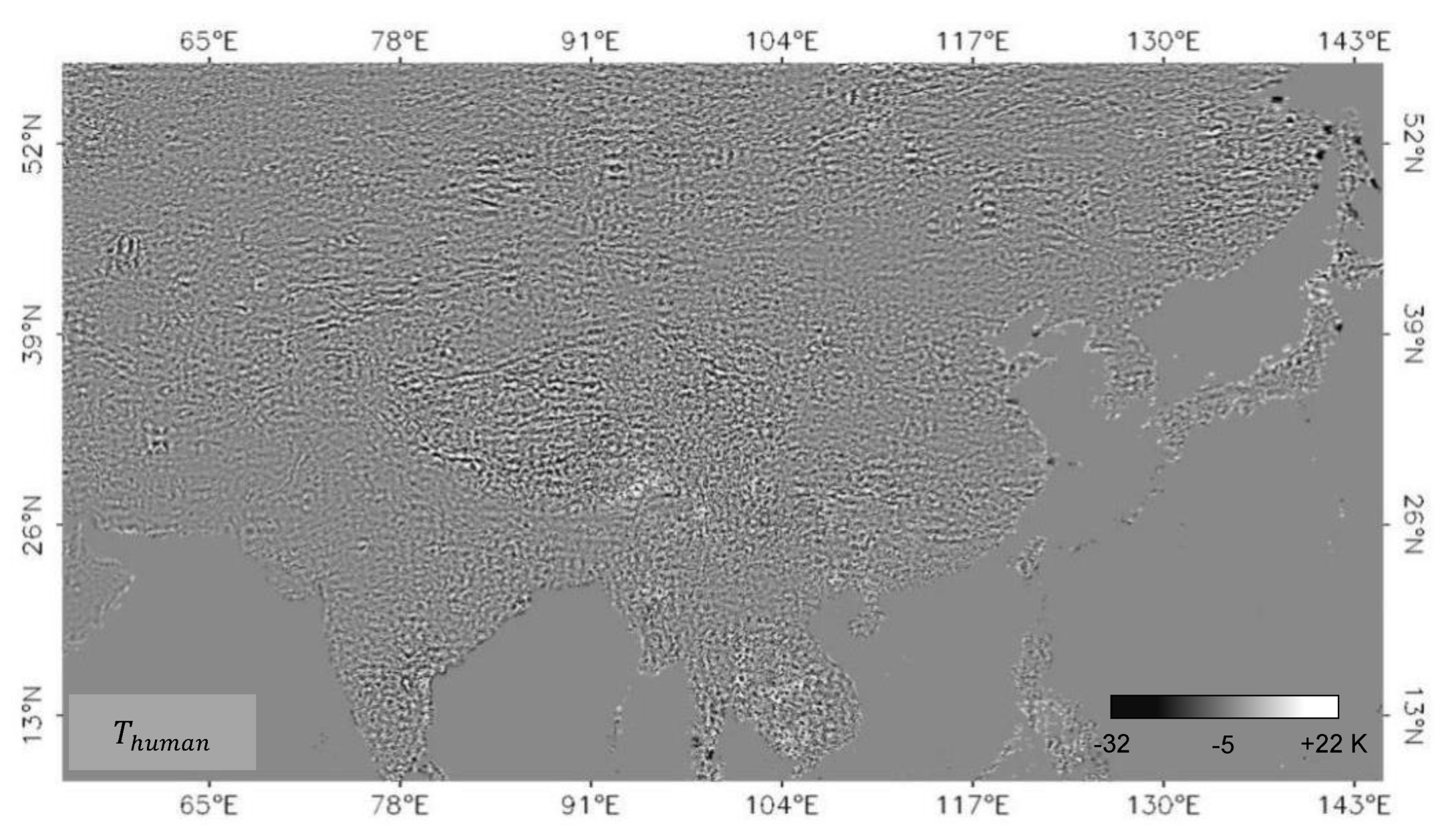
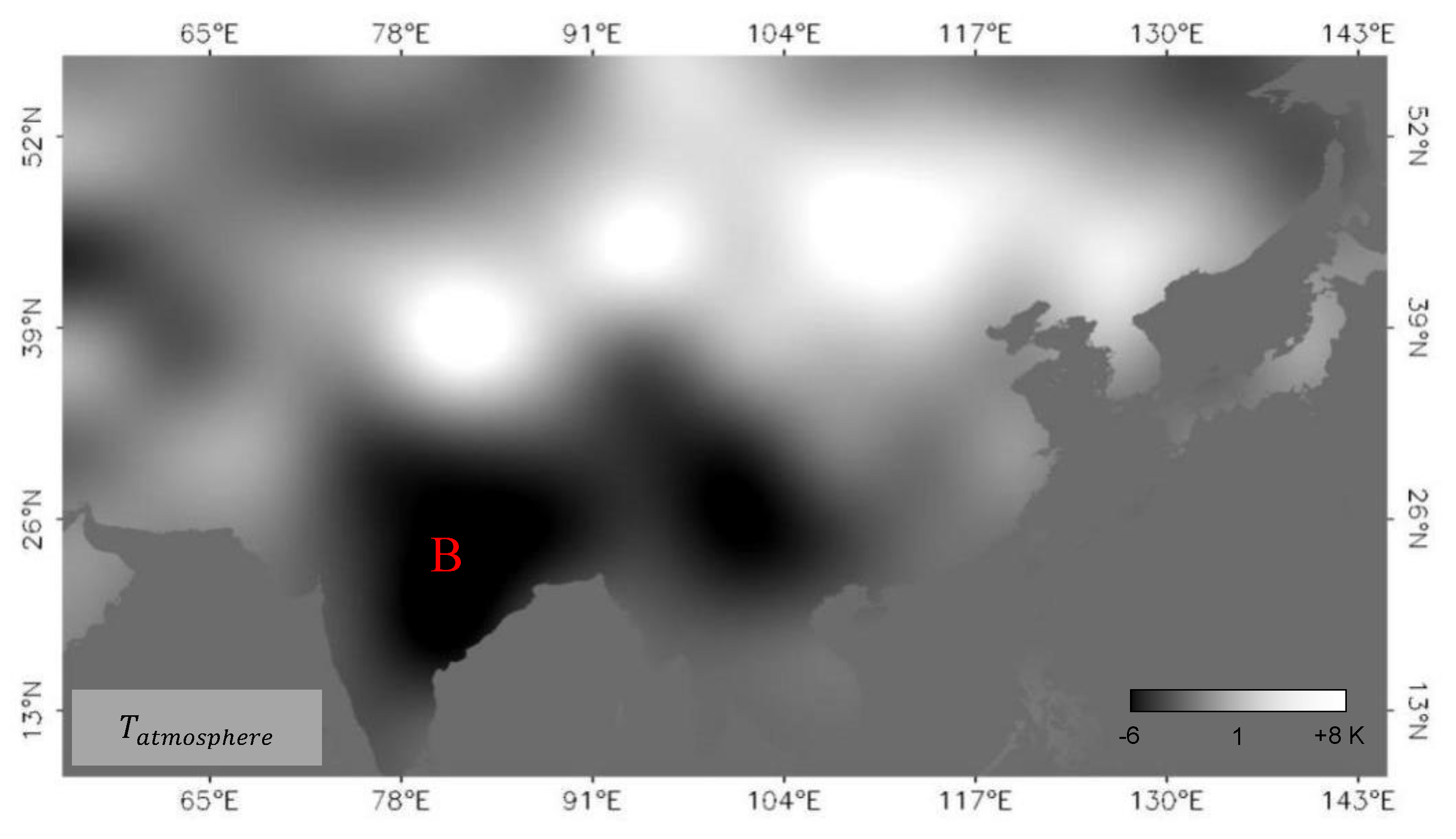
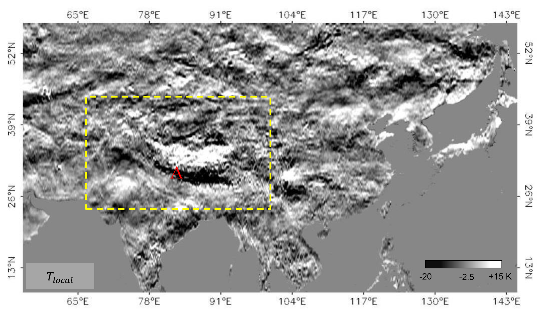
Appendix D. Spatial Distribution of Land Surface Temperature and Its Components


References
- Geller, R.J. Earthquake prediction: A critical review. Geophys. J. Int. 1997, 131, 425–450. [Google Scholar] [CrossRef] [Green Version]
- Geller, R.J.; Jackson, D.D.; Kagan, Y.Y.; Mulargia, F. Earthquakes Cannot Be Predicted. Science 1997, 275, 1616–1620. [Google Scholar] [CrossRef] [Green Version]
- Ohnaka, M. The Physics of Rock Failure and Earthquakes; Cambridge University Press: New York, NY, USA, 2013. [Google Scholar]
- Vallianatos, F.; Georgios, C. A Complexity View into the Physics of the Accelerating Seismic Release Hypothesis: Theoretical Principles. Entropy 2018, 20, 754. [Google Scholar] [CrossRef] [Green Version]
- Song, D.; Xie, R.; Zang, L.; Yhi, J.; Qin, K.; Shan, X.; Cui, J.; Wang, B. A New Algorithm for the Characterization of Thermal Infrared Anomalies in Tectonic Activities. Remote Sens. 2018, 10, 1941. [Google Scholar] [CrossRef] [Green Version]
- Jiao, Z.-H.; Zhao, J.; Shan, X. Pre-seismic anomalies from optical satellite observations: A review. Nat. Hazards Earth Syst. Sci. 2018, 18, 1013–1036. [Google Scholar] [CrossRef] [Green Version]
- Varotsos, P.; Eftaxias, K.; Vallianatos, F.; Lazaridou, M. Basic principles for evaluating an earthquake prediction method. Transl. World Seismol. 1995, 23, 1295–1298. [Google Scholar] [CrossRef] [Green Version]
- Qiang, Z.; Xu, X.; Dian, C. Satellite infrared thermos-anomaly: Earthquake imminent precursor. Chin. Sci. Bull. 1990, 35, 1324–1327. [Google Scholar]
- Qiang, Z.J.; Kong, L.C.; Wang, Y.P. Earth gas emission, infrared thermo-anomaly and seismicity. Chin. Sci. Bull. 1992, 24, 2259–2262. [Google Scholar]
- Tronin, A.A. Satellite thermal survey—A new tool for the studies of seismoactive regions. Int. J. Remote Sens. 1996, 17, 1439–1455. [Google Scholar] [CrossRef]
- Tronin, A.A. Remote sensing and earthquakes: A review. Phys. Chem. Earth 2006, 31, 138–142. [Google Scholar] [CrossRef]
- Tronin, A.A. Satellite Remote Sensing in Seismology: A Review. Remote Sens. 2010, 2, 124–150. [Google Scholar] [CrossRef] [Green Version]
- Tronin, A.A.; Hayakawa, M.; Molchanov, O.A. Thermal IR satellite data application for earthquake research in Japan and China. J. Geodyn. 2002, 33, 519–534. [Google Scholar] [CrossRef]
- Gorny, V.I.; Salman, A.G.; Tronin, A.A.; Shilin, B.B. Outgoing infrared radiation of the earth as an indicator of seismic activity. DoSSR 1988, 301, 67–69. [Google Scholar]
- Ouzounov, D.; Freund, F.T. Mid-infrared emission prior to strong earthquakes analyzed by remote sensing data. Adv. Space Res. 2004, 33, 268–273. [Google Scholar] [CrossRef]
- Ouzounov, D.; Liu, D.; Kang, C.; Guido, C.; Menas, K.; Patrick, T. Outgoing long wave radiation variability from IR satellite data prior to major earthquakes. Tectonophysics 2007, 431, 211–220. [Google Scholar] [CrossRef]
- Tramutoli, V.; Cuomo, V.; Filizzola, C.; Pergola, N.; Pietrapertosa, C. Assessing the potential of thermal infrared satellite surveys for monitoring seismically active areas: The case of Kocaeli (Izmit) earthquake, August 17, 1999. Remote Sens. Environ. 2005, 96, 409–426. [Google Scholar] [CrossRef]
- Freund, F. Pre-earthquake signals-Part I: Deviatoric stresses turn rocks into a source of electric currents. Nat. Hazards Earth Syst. Sci. 2007, 7, 535–541. [Google Scholar] [CrossRef] [Green Version]
- Freund, F. Pre-earthquake signals-Part II: Flow of battery currents in the Crust. Nat. Hazards Earth Syst. Sci. 2007, 7, 543–548. [Google Scholar] [CrossRef] [Green Version]
- Freund, F. Pre-earthquake signals: Underlying physical processes. J. Asian Earth Sci. 2011, 41, 343–400. [Google Scholar] [CrossRef]
- Freund, F.; Takeuchi, A.; Lau, B.W.S.; Al-Manaseer, A.; Fu, C.C.; Bryant, N.A.; Ouzounov, D. Stimulated infrared emission from rocks: Assessing a stress indicator. eEarth 2007, 2, 1–10. [Google Scholar] [CrossRef] [Green Version]
- Geng, N.G.; Cui, C.Y.; Deng, M.D. Remote sensing detection of rock fracturing experiment and the beginning of remote rock mechanics. Acta Seismol. Sin. 1992, 14, 645–652. (In Chinese) [Google Scholar]
- Saraf, A.K.; Rawat, V.; Choudhury, S.; Dasgupta, S.; Das, J. Advances in understanding of the mechanism for generation of earthquake thermal precursors detected by satellites. Int. J. Appl. Earth Obs. Geoinf. 2009, 11, 373–379. [Google Scholar] [CrossRef]
- Eleftheriou, C.; Filizzola, N.; Genzano, T.; Lacava, M.; Lisi, R.; Paciello, N.; Pergola, F.; Vallianatos, V. Tramutoli. Long-Term RST Analysis of Anomalous TIR Sequences in Relation with Earthquakes Occurred in Greece in the Period 2004–2013. Pure Appl. Geophys. 2016, 173, 285–303. [Google Scholar] [CrossRef] [Green Version]
- Bhardwaj, A.; Singh, S.; Sam, L.; Bhardwaj, A.; Martín-Torres, F.J.; Singh, A.; Kumar, R. MODIS-based estimates of strong snow surface temperature anomaly related to high altitude earthquakes of 2015. Remote Sens. Environ. 2017, 188, 1–8. [Google Scholar] [CrossRef]
- Blackett, M.; Wooster, M.; Malamud, B. Exploring land surface temperature earthquake precursors: A focus on the Gujarat (India) earthquake of 2001. Geophys. Res. Lett. 2011, 38. [Google Scholar] [CrossRef]
- Chen, S.Y.; Ma, J.; Liu, P.X.; Liu, L.Q.; Ren, Y.Q. Exploring the current tectonic activity with satellite remote sensing thermal information: A case of the Wenchuan earthquake. Seismol. Geol. 2014, 36, 775–793. [Google Scholar]
- Liu, J.; Chen, J.I.; Zhang, J.Y.; Zhang, P.Z.; Wei, W. Tectonic setting and general features of coseismic rupture of the 25 April, 2015 Mw 7.8 Gorkha Nepal earthquake (in Chinese). Chin. Sci. Bull. 2015, 60, 2640–2655. [Google Scholar] [CrossRef] [Green Version]
- Yang, X.-P.; Wu, G.; Chen, L.-C.; Li, C.-Y.; Chen, X.-L. The seismogenic structure of the April 25, 2015 MW7.8 Nepal earthquake in the southern margin of Qinghai-Tibetan Plateau. Chin. J. Geophys. 2016, 59, 2528–2538. [Google Scholar]
- Nandita, D.G. Atmospheric changes observed during April 2015 Nepal earthquake. J. Atmos. Sol. Terr. Physics. 2016, 140, 16–22. [Google Scholar]
- Chakraborty, S.; Sasmal, S.; Chakrabarti, S.K.; Bhattacharya, A. Observational signatures of unusual outgoing longwave radiation (OLR) and atmospheric gravity waves (AGW) as precursory effects of May 2015 Nepal earthquakes. J. Geodyn. 2018, 113, 43–51. [Google Scholar] [CrossRef]
- Molnar, P.; Tapponnier, P. Cenozoic tectonics of Asia: Effects of a continental collision. Science 1975, 189, 419–426. [Google Scholar] [CrossRef] [PubMed]
- Nakata, T. Active faults of the Himalaya of India and Nepal. GSA Spec. Pap. 1989, 232, 243–261. [Google Scholar]
- Ni, J.; Barazangi, M. Seismotectonics of the Himalayan Collision Zone: Geometry of the underthrusting Indian Plate beneath the Himalaya. J. Geophys. Res. Solid Earth 1984, 89, 1147. [Google Scholar] [CrossRef]
- Brown, L.; Zhao, W.; Nelson, K.; Hauck, M.; Alsdorf, D.; Ross, A.; Cogan, M.; Clark, M.; Liu, X.; Che, J. Bright spots, Structure, and Magmatism in Southern Tibet from INDEPTH Seismic Reflection Profiling. Science 1996, 274, 1688–1690. [Google Scholar] [CrossRef]
- Zhang, X.; Xu, L.-S. Inversion of the apparent source time functions for the rupture process of the Nepal Ms8.1 earthquake. Chin. J. Geophys. 2015, 58, 1881–1890. (In Chinese) [Google Scholar]
- Lay, T.; Ye, L.; Koper, K.D.; Kanamori, H. Assessment of teleseismically-determined source parameters for the April 25, 2015 MW 7.9 Gorkha, Nepal earthquake and the May 12, 2015 MW 7.2 aftershock. Tectonophysics 2017, 714, 4–20. [Google Scholar] [CrossRef]
- Denolle, M.A.; Fan, W.; Shearer, P.M. Dynamics of the 2015 M7.8 Nepal earthquake. Geophys. Res. Lett. 2015, 42, 7467–7475. [Google Scholar] [CrossRef]
- Wan, Z.; Li, Z.L. A physics-based algorithm for retrieving land surface emissivity and temperature from EOS/MODIS data. IEEE Trans. Geosci. Remote Sens. 1997, 35, 980–996. [Google Scholar]
- Wan, Z.M. New refinements and validation of the MODIS Land Surface Temperature/Emissivity products. Remote Sens. Environ. 2008, 112, 59–74. [Google Scholar] [CrossRef]
- Wan, Z.M.; Zhang, Y.L.; Zhang, Q.H.; Li, Z. Validation of the land surface temperature products retrieved from Terra Moderate Resolution Imaging Spectroradiometer data. Remote Sens. Environ. 2002, 83, 163–180. [Google Scholar] [CrossRef]
- Li, J.; Tang, Y. Application of Wavelet Analyses; Chongqing University Press: Chongqing, China, 1999. (In Chinese) [Google Scholar]
- Mallat, S. A theory of multi-resolution signal decomposition: The wavelet representation. IEEE Trans. PAMI 1989, 11, 674–693. [Google Scholar] [CrossRef] [Green Version]
- Wu, L.; Cui, C.; Geng, N.; Wang, J. Remote sensing rock mechanics (RSRM) and associated experimental studies. Int. J. Rock Mech. Min. Sci. 2000, 37, 879–888. [Google Scholar] [CrossRef]
- Yin, J.Y.; Fang, Z.F.; Qian, J.D.; Deng, M.D.; Geng, N.G.; Hao, J.S.; Wang, Z.; Ji, Q.Q. Research on the application of infrared remote sensing in earthquake prediction and its physical mechanism. Earthq. Res. China 2000, 16, 140–148. [Google Scholar]
- Pulinets, S.; Ouzounov, D.; Karelin, A.; Boyarchuk, K.; Pokhmelnykh, L. The physical nature of thermal anomalies observed before strong earthquakes. Phys. Chem. Earth Part A/B/C 2006, 31, 143–153. [Google Scholar] [CrossRef]
- Ren, Y.; Chen, S.; Ma, J. Variation of land surface temperature in Yilan-Yitong fault zone of northeastern China. Acta Seismol. Sin. 2012, 34, 698–705. [Google Scholar]
- Chen, S.; Liu, P.; Guo, Y.; Liu, L.; Ma, J. Co-Seismic Response of Bedrock Temperature to the Ms6.3 Kangding Earthquake on 22 November 2014 in Sichuan, China. Pure Appl. Geophys. 2019, 176, 97–117. [Google Scholar] [CrossRef]
- Chen, S.Y.; Liu, L.; Liu, P.; Ma, J.; Ghen, G. Theoretical and experimental study on relationship between stress-strain and temperature variation. Sci. China Ser. D Earth Sci. 2009, 52, 1825–1834. [Google Scholar] [CrossRef]
- Liu, P.; Chen, S.; Liu, L.; Chen, G.; Ma, J. An experiment on the infrared radiation of surficial rocks during deformation. Seismol. Geol. 2004, 26, 502–511, (In Chinese with English abstract). [Google Scholar]
- Yang, X.; Lin, W.; Tadai, O.; Zeng, X.; Yu, C.; Yeh, E.-C.; Li, H.; Wang, H. Experimental and numerical investigation of the temperature response to stress changes of rocks. J. Geophys. Res. Solid Earth 2017, 122, 5101–5117. [Google Scholar] [CrossRef] [Green Version]
- Chui, C.K. An Introduction to Wavelets; Academic Press: San Diego, CA, USA, 1992. [Google Scholar]
- Daubechies, I. Ten Lectures on Wavelets; SIAM Press: Philadelphia, PA, USA, 1992. [Google Scholar]
- Boggess, A.; Narcowich, F.J. A First Course in Wavelets with Fourier Analysis; John Wiley & Sons, Inc.: Hoboken, NJ, USA, 2009. [Google Scholar]
- Chen, S.-Y.; Ma, J.; Liu, P.-X.; Liu, L.-Q. A study on the normal annual variation field of land surface temperature in China. Chin. J. Geophys. 2009, 52, 962–971. [Google Scholar] [CrossRef]


| Study Area | Totals | Non–Smoothed | Smoothed | ||||||
|---|---|---|---|---|---|---|---|---|---|
| Mean | Std a | Max | Min | Mean | Std | Max | Min | ||
| No. 1 | 641 | 0.11 | 1.42 | 3.91 | −4.51 | 0.11 | 0.64 | 2.02 | −1.66 |
| No. 2 | 641 | −0.03 | 1.39 | 3.71 | −4.35 | −0.02 | 0.62 | 1.57 | −1.63 |
| No. 3 | 641 | −0.17 | 1.55 | 4.61 | −4.66 | −0.17 | 0.75 | 1.37 | −2.86 |
| No. 4 | 641 | −0.20 | 1.65 | 3.64 | −5.83 | −0.20 | 0.95 | 1.37 | −4.60 |
| No. 5 | 641 | 0.11 | 1.42 | 3.91 | −4.51 | 0.04 | 0.37 | 1.27 | −1.28 |
© 2020 by the authors. Licensee MDPI, Basel, Switzerland. This article is an open access article distributed under the terms and conditions of the Creative Commons Attribution (CC BY) license (http://creativecommons.org/licenses/by/4.0/).
Share and Cite
Chen, S.; Liu, P.; Feng, T.; Wang, D.; Jiao, Z.; Chen, L.; Xu, Z.; Zhang, G. Exploring Changes in Land Surface Temperature Possibly Associated with Earthquake: Case of the April 2015 Nepal Mw 7.9 Earthquake. Entropy 2020, 22, 377. https://doi.org/10.3390/e22040377
Chen S, Liu P, Feng T, Wang D, Jiao Z, Chen L, Xu Z, Zhang G. Exploring Changes in Land Surface Temperature Possibly Associated with Earthquake: Case of the April 2015 Nepal Mw 7.9 Earthquake. Entropy. 2020; 22(4):377. https://doi.org/10.3390/e22040377
Chicago/Turabian StyleChen, Shunyun, Peixun Liu, Tao Feng, Dong Wang, Zhonghu Jiao, Lichun Chen, Zhengxuan Xu, and Guangze Zhang. 2020. "Exploring Changes in Land Surface Temperature Possibly Associated with Earthquake: Case of the April 2015 Nepal Mw 7.9 Earthquake" Entropy 22, no. 4: 377. https://doi.org/10.3390/e22040377