Use of Infrared Satellite Observations for the Surface Temperature Retrieval over Land in a NWP Context


CNRM, Université de Toulouse, Météo-France, CNRS, Toulouse, France
*
Author to whom correspondence should be addressed.
†
These authors contributed equally to this work.
Remote Sens. 2019, 11(20), 2371; https://doi.org/10.3390/rs11202371
Submission received: 2 September 2019
/
Revised: 3 October 2019
/
Accepted: 9 October 2019
/
Published: 12 October 2019
(This article belongs to the Section Atmospheric Remote Sensing)
Abstract
:In Numerical Weather Prediction (NWP), an accurate description of surface temperature is needed to assimilate satellite observations. These observations produced by infrared and microwave sensors, help retrieving good quality land surface temperature (LST) by using surface sensitive channels and emissivity atlases. This work is a preparatory step in order to assimilate LSTs in Météo-France NWP models surface analysis. We focus on IASI and SEVIRI sensors. The first part of this work aims at comparing the SEVIRI retrieved LST to local observations from two stations included in the meso-scale AROME-France domain over four periods from different seasons. Diurnal cycles of local LST and SEVIRI LST show a good agreement especially for the summer period. Averaged biases show seasonal variability and are smaller during Winter and Autumn with less than 1 K values for both stations. The second part of the study deals with the comparison of LST values retrieved from different infrared sensors in AROME-France model. First results show encouraging agreement between both LSTs. A comparison during Autumn period for clear sky conditions reveals an almost null bias and a standard deviation of about 1.6 K. More detailed comparisons were performed over contrasted seasons with a special attention to diurnal cycles for both sensors. A better agreement is noticed during nighttime. The last step of this inter-comparison was to study the simulation of SEVIRI and IASI brightness temperatures by using a fast radiative transfer model. Thus, several simulations have been run covering various dates from different seasons by daytime and nighttime using SEVIRI LSTs, IASI LSTs and AROME-France model LSTs. Simulated brightness temperatures were then compared to observations. As expected, the best simulations are the ones using the LST retrieved from the sensor for which simulations are performed. However, the LST retrieved from another sensor provides better simulations than the predicted LST from the model especially during nighttime. For IASI simulations, SEVIRI LSTs increase RMSE by 0.2 K to 0.9 K compared to IASI LSTs for nighttime case and by around 1.5 K for daytime.

1. Introduction
The surface temperature is a key parameter in surface analysis. However, it is difficult to predict it with good precision over land due to its large diurnal variability and its dependence upon land cover and surface emissivity that have high spatial and temporal variability over land and might vary even over similar land covers. Most surface schemes in NWP use analyzed surface temperature based on 2-m air temperature observations [1,2]. However, over continents, the Land Surface Temperatures (LSTs) and Land Surface Emissivities (LSEs) have higher spatial and temporal variabilities compared to 2-m air temperatures.
Moreover, an accurate description of surface properties (skin temperature and surface emissivity) is necessary to assimilate satellite observations sensitive to the surface, both in the thermal infrared (∼3 m–14 m) and in the microwave (∼0.16 cm–1.3 cm) spectra. The description of surface temperature faces several challenges over land, because of it high variability in space and time and the difficulties in estimating surface emissivities.
New approaches have been developed in order to retrieve LSTs based on remotely sensed observations [3]. These approaches use window channels, which are particularly sensitive to surface radiation, and are less impacted by the atmosphere. These retrieved LSTs enable NWP models to assimilate more satellite channels sensitive to the surface and the lower atmosphere, through a better observation simulation. Previous studies have shown the benefits of retrieved LSTs in assimilating more satellite channels compared to the use of model LST which is analyzed from the 2-m air temperature [4].
Despite the fact that the assimilation of the retrieved surface temperature has shown benefits over oceans [5], it has to face a number of challenges when considering surface sensitive channels over land. For these window channels, the surface emissivity and skin temperature uncertainties have significant impact. However, new methods were brought to NWP models in order to take into account the variations in land surface temperature and emissivity which makes the assimilation of surface sensitive channels possible over land [6]. First results showed improvements in low-level temperature and mid-tropospheric water vapor.
Recent studies have considered assimilating satellite derived LSTs over land. In fact, assimilating geostationary satellites derived LSTs in a land surface model with nighttime observations [7] have shown encouraging results at global scale both for the surface scheme and the atmospheric forecasts. Moreover, the assimilation of polar-orbiting satellite retrieved LSTs, when satellite data are available near the peak of diurnal LST, considerably improved the estimation of the fields of energy balance components and surface control on evaporation [8].
For microwave sensors, the radiative transfer equation is inverted using the model surface temperature to retrieve the LSE [9]. For infrared sensors, such as SEVIRI [10] and IASI [11], the observed brightness temperatures in window channels are used together with an emissivity atlas in order to retrieve LSTs, by solving the inverse problem of the radiative transfer equation. In fact, different methods exist for the LST retrieval [12]. It is possible to retrieve the surface temperature with or also without a known emissivity. In case of unknown emissivity, different algorithms allow the retrieval of the emissivity and the land surface temperature such as the TES (temperature and emissivity separation) method [13], the artificial neural network [14], the two-temperature method [15] or the Day and Night method [16]. In case of a known surface emissivity, different methods exist such as the split-window algorithm [17] or methods based on multi-angular, multi-channel [18] or mono-channel approaches [19]. At Météo-France, the adopted method for operational LST retrieval is the mono-channel with known emissivity [20,21].
The current study consists in a preliminary step in order to assimilate LST in the surface analysis of Météo-France NWP models. As explained above, the current surface data assimilation in Météo-France NWP systems uses an Optimal Interpolation with 2-m air temperature and relative humidity observations which provide indirect information on land surface temperature. The objectives in near future at Météo-France are to also assimilate LSTs retrieved from infrared sounders in the surface analysis. Moreover, in the atmospheric analysis, LSTs are retrieved from infrared sounders for the assimilation of their brightness temperatures, but with no feed-back to the surface analysis. Our goal is thus to prepare the assimilation of these retrieved LST in the surface data assimilation scheme. Here, we focus on SEVIRI, IASI and model LSTs in order to study the agreement between them, evaluate their impact on the radiative transfer simulation and their potential relevance for their use in the surface analysis.
The retrieved LSTs from SEVIRI are first assessed with local observations and with the AROME-France model forecast. The agreement between LSTs retrieved from two spaceborne sensors (SEVIRI, IASI) and with the AROME-France model over land is then examined. Finally the impact of using LSTs retrieved from one sensor on the observation simulation of the second instrument is evaluated to assess the possible synergy between infrared sensors to define a common LST.
In Section 2, we introduce the AROME-France operational model and the retrieval method. Section 3 evaluates the agreement between SEVIRI LSTs and local LSTs observed at two instrumented sites, compared to model LSTs. Section 4 summarizes the results of the comparison between SEVIRI LST and IASI LST, over different 2-month periods chosen during the four seasons. Section 5 presents the results of radiance simulation with the radiative transfer model RTTOV, for IASI and SEVIRI sensors while using three different values of LST: two retrieved from both sensors and one predicted by the surface model. Finally, conclusions and future work are discussed in Section 6.
2. LST Retrieval in AROME-France
2.1. AROME-France Model
AROME-France (Applications de la Recherche à l’Opérationnel à Méso-Echelle) is the meso-scale non hydrostatic model of Météo-France, operational since December 2008 [22]. AROME-France merges a part of the physical package of Meso-NH research model [23] with the non-hydrostatic version of the ALADIN model dynamics [24]. Table 1 summarizes the main characteristics of the operational version since 2015.
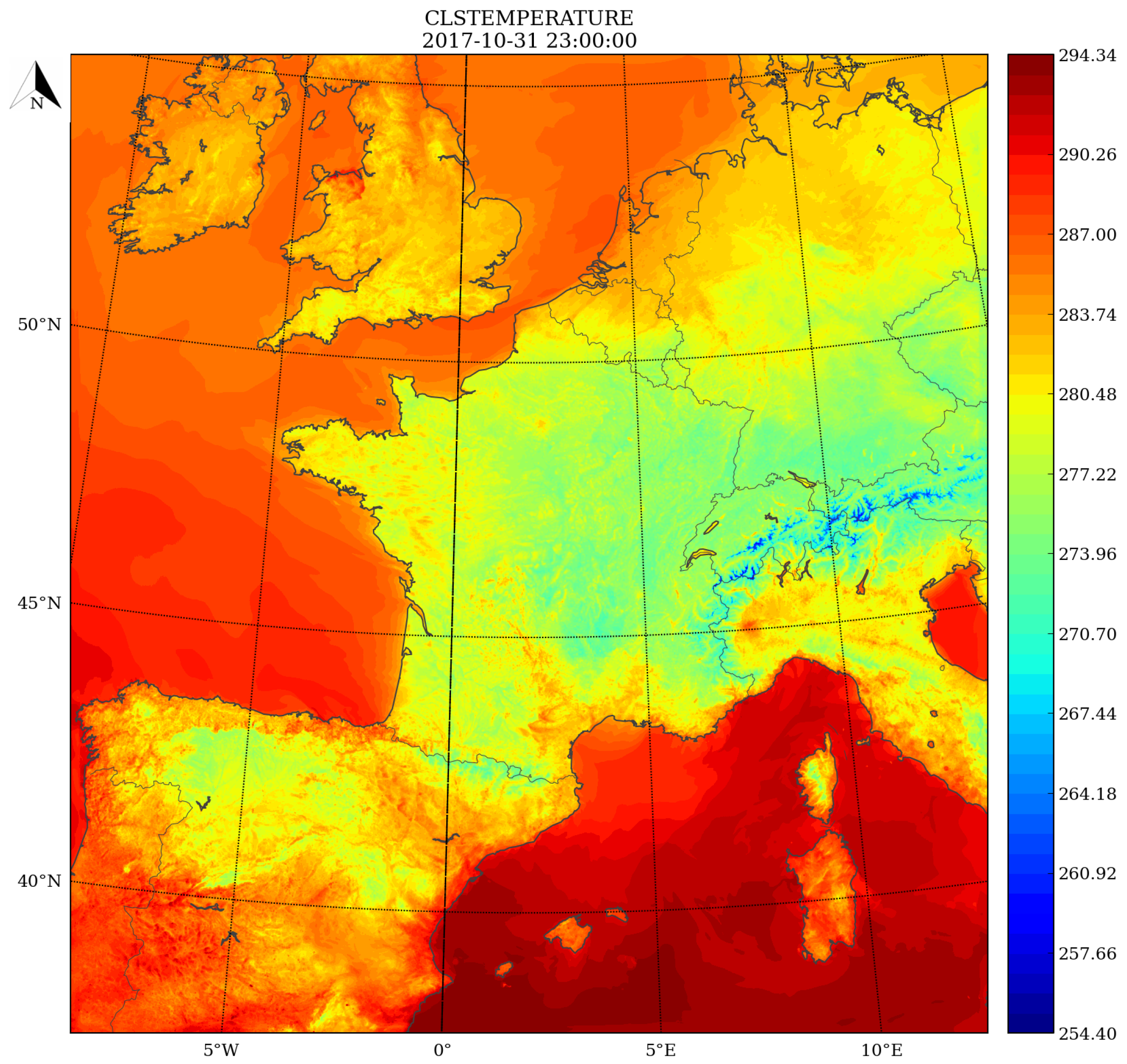
The domain of AROME-France operational model extends from −12.45E to 16.67E and from 37.26N to 55.69N with 1.3 km of horizontal resolution as shown in Figure 1 representing the 2-m air temperature field on the 31 October 2017, 23 UTC.
For the surface component, AROME-France is coupled to SURFEX (SURFace EXternalized) model which is a surface modelling platform. SURFEX divides the surface into four tiles: Nature, Town, Lake and Sea [25]. Over the nature tile, fields of soil temperatures and water contents (surface and deep layers, liquid and solid parts for water) are prognostic variables. These fields are analyzed with a 1D Optimal Interpolation (OI). The screen level parameters ( 2-m air temperature and relative humidity) are analyzed using a 2D Optimal Interpolation with model fields. Then the increments of the 2-m air temperature and the relative humidity are used as pseudo-observations in the soil analysis.
AROME-France model is initialized for its atmospheric component with a 3D-Var with 1-h cycles assimilation system [26] derived from the Météo-France global ARPEGE variational assimilation system and adapted to its high resolution. Different types of observations are assimilated such as in-situ observations over land and sea, GNSS Zenithal Total Delays and weather radars which improve the initial state of the model for wind and humidity in the precipitating systems. Satellite observations are also assimilated and among them IASI (44 assimilated channels over sea and 8 assimilated channels over land) [27] and SEVIRI (6 assimilated channels over sea and 5 assimilated channels over land) observations.
2.2. Satellite Data
The Infrared Atmospheric Sounding Interferometer (IASI) [11] is a hyperspectral infrared sounder on board Metop-A, Metop-B and Metop-C (launched on 7 November 2018) satellites on a low polar Earth orbit. IASI sounds the atmosphere with a vertical resolution of 1 km and an accuracy of 1 K for temperature and provides information on temperature and humidity profiles. As an infrared sensor, IASI is also sensitive to clouds and to the surface. In addition, IASI detects with accuracy the atmospheric composition of different chemical components such as stratospheric ozone.
IASI observes the Earth in 8461 channels every 0.25 cm. The IASI field of view consists of a 2 × 2 matrix of four circular pixels of 12 km diameter at nadir. The IASI swath width is 2200 km.
The Spinning Enhanced Visible and Infrared Imager (SEVIRI) [10] is on board MSG satellites on a geostationary orbit at about 36,000 km above equator. It observes the Earth with 12 channels from visible to infrared, among which 8 thermal infrared channels. Table 2 presents the main characteristics of IASI and SEVIRI sensors.
2.3. LST Retrieval
Thermal exchanges at the Earth’s surface maintain the radiative energy balance between the Earth and the atmosphere. Equation (1) describes the surface-atmosphere radiative interactions [21]:
where is the observed radiance, is the land surface emissivity, is the incidence angle, is the Planck function, is the land surface temperature, is the atmospheric transmittance, and are respectively the up-welling and the down-welling radiances for the channel .
AROME-France uses the RTTOV radiative transfer model [28]. It was initially developed by ECMWF (European Centre for Medium-Range Weather Forecasts) in the 1990’s in order to enable the direct assimilation of satellite radiances. In 1998, the EUMETSAT-funded NWP SAF (Numerical Weather Prediction Satellite Application Facility) took in charge the development of RTTOV with contributions from ECMWF, Météo-France, Met Office and DWD. Nowadays, RTTOV can simulate around 90 sensors in infrared, micro-wave and visible bandwidths onboard around 50 satellites. RTTOV allows, besides the forward model, the perturbation of input variables such as surface type and skin temperature and the computation of the Jacobian matrix.
For the LST retrieval, we are faced to the inverse problem, knowing the observed radiance and in our case the surface emissivity, defined by an emissivity atlas. The Equation (1) becomes then [20]:
The method used for operational LST retrievals at Météo-France is the mono-channel with known emissivity method [20,21]. This method uses a single selected window channel in order to retrieve LST and needs some a priori information such as the atmospheric transmittance and the surface emissivity. This latter can be considered from emissivity atlases. In fact, different emissivity atlases are used for different sensors. During this study, we have used the operational version of AROME-France that runs the RTTOV v11 for the retrievals. For IASI LST retrieval, the emissivity is defined with the infrared atlas of the University of Wisconsin which is a global monthly infrared land surface emissivity database [29] with high spectral resolution from 3.6 m to 14.3 m and a spatial resolution of 0.05. This database was produced using principal component analysis regression of high spectral resolution laboratory measurements of selected materials from MODIS/UCSB (University of California, Santa Barbara) and ASTER emissivity libraries and CIMSS (Cooperative Institute of Meteorological Satellite Studies) Baseline Fit global infrared land surface emissivity database [30]. At Météo-France, the Winsconsin University infrared surface emissivity atlas has been calculated based on UW atlas version of 2007 with a spatial resolution of 0.1 due to operational constraints. The inversion uses the window channel number 1194 at 10.6 m (wave number of 943.25 cm). This channel was selected among other IASI window channels for the operational retrievals in AROME-France model [4]. Regarding the retrieval of SEVIRI LST, it uses the mono channel method with known emissivity coming from the Satellite Application Facility on Land Surface Analysis (LSA-SAF) data [31]. In fact, we use the LSA-SAF LSEs in order to produce monthly mean values of emissivity at a spacial resolution of 0.1. These mean values are used further for the operational retrievals of SEVIRI LSTs. The current version of monthly mean emissivities used for the operational retrievals of SEVIRI LSTs has been calculated based on 2017 LSA-SAF LSEs. The channel used for the LST retrieval is the window channel at 10.8 m. This channel was selected for operational retrievals based on a previous study [21].
Since infrared observed radiances can be contaminated by clouds, the retrievals are considered only in clear sky conditions. For IASI observations, the cloud cover information is produced by the Advanced Very High Resolution Radiometer (AVHRR) instrument which corresponds to the percentage of cloudy AVHRR pixels inside the IASI FOV (Field of View). AVHRR is on board NOAA and Metop satellites and has a high spatial resolution of 1 km at nadir. For SEVIRI observations, the cloud cover information is based on a cloud detection algorithm that uses the top of cloud pressure information [32] and the RTTOV model in order to simulate the observed radiances under different cloud cover conditions. The surface temperature retrieval is also sensitive to the atmospheric transmittance as shown in Equation (2). In fact, the retrievals are only performed when atmospheric transmittance is above 0.5. This value was set as transmittance threshold for operational retrievals in AROME-France model [33].
3. Comparison to Local Data
The aim of this section is to evaluate SEVIRI LSTs agreement with in-situ observations. Therefore, we compared the SEVIRI retrieved LSTs and the forecasted LSTs from the model to local data in France and Portugal. Two sites located in the AROME-France domain where observed surface temperature is available at an hourly temporal frequency were chosen for this study: Toulouse station in France and Evora station in Portugal. SEVIRI observes the Earth with a 15 min temporal resolution but the comparison is limited to clear sky SEVIRI observations taken on sharp hours only. Four periods of two months each were considered for the comparisons: spring (April & May 2018), summer (July & August 2018), autumn (October & November 2018) and winter (January & February 2018).
3.1. Local Data Acquisition
The first comparison uses data from Toulouse station (1.37E; 43.57N) which is located in the Occitany region, south-west of France. This region has a warm and relatively dry summer and a mild and wet winter. The station is a part of Meteopole-Flux project [34] which aims to build a long-term survey of different variables such as the surface energy balance in a grassland zone in the suburb areas of Toulouse. The station is equipped among others with a KT15.85D infrared radiation radiometer. The spectral band of this instrument ranges from 9.6 m to 11.5 m.
The second comparison uses Evora station data. Evora station is one of four KIT (Karlsruhe Institute of Technology) LST validation stations of the LSA-SAF which are located in wide homogeneous areas and equipped with the KT-15.85 IIP infrared radiometer with a spectral band from 9.6 m to 11.5 m [35,36]. Evora LST validation station is located at about 12 km south-west of Evora city in Portugal (8.0034W; 38.5403N). The main vegetation type is grassland and evergreen oak trees. The climate is characterized by a dry and warm summer, and a wet and cold winter season.
For both stations, the local LSTs measured with the KT15 infrared radiometers were compared with the mean SEVIRI LSTs and the mean model LSTs within a radius of 4.5 km.
3.2. Results of Comparison
This section presents the results of comparing SEVIRI LSTs with local LSTs for Toulouse and Evora stations during spring, summer, fall and winter periods. The comparison includes the diurnal cycles and also the statistics of differences in terms of mean difference and standard deviation. The comparison includes also the LST forecast by the AROME-France/SURFEX model.
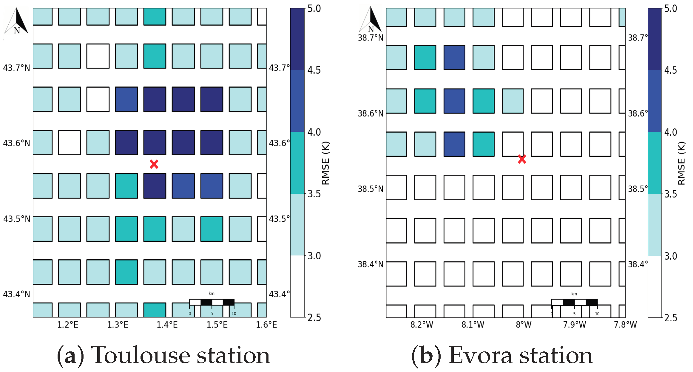
While LST validation Evora station is situated in a homogeneous area in terms of soil cover, the Toulouse station is situated in an urban area at the west side of Toulouse between the town and the lake of La Ramée. Since different soil covers have different radiative properties, we decided to compare the soil occupation observed by the station pyrometer and the SEVIRI pixels. For Toulouse station, on one side, the radiometer is observing a small homogeneous field of grass inside the Toulouse Météopole, and on the other side, SEVIRI pixels cover different large areas including various proportions of town and nature soil occupation. Worth to note that some of the nearest pixels of SEVIRI to the observation station cover the urban area of southern part of Toulouse (Figure 2a) which presents different soil covers than the area observed by the radiometer. For Evora station, the nearest SEVIRI pixels to the station observe similar soil cover as the radiometer (Figure 2b).
Figure 2b shows higher values of RMSE in north-west of Evora station. This area is characterized by a different soil occupation with forested area which induces different emissivities.
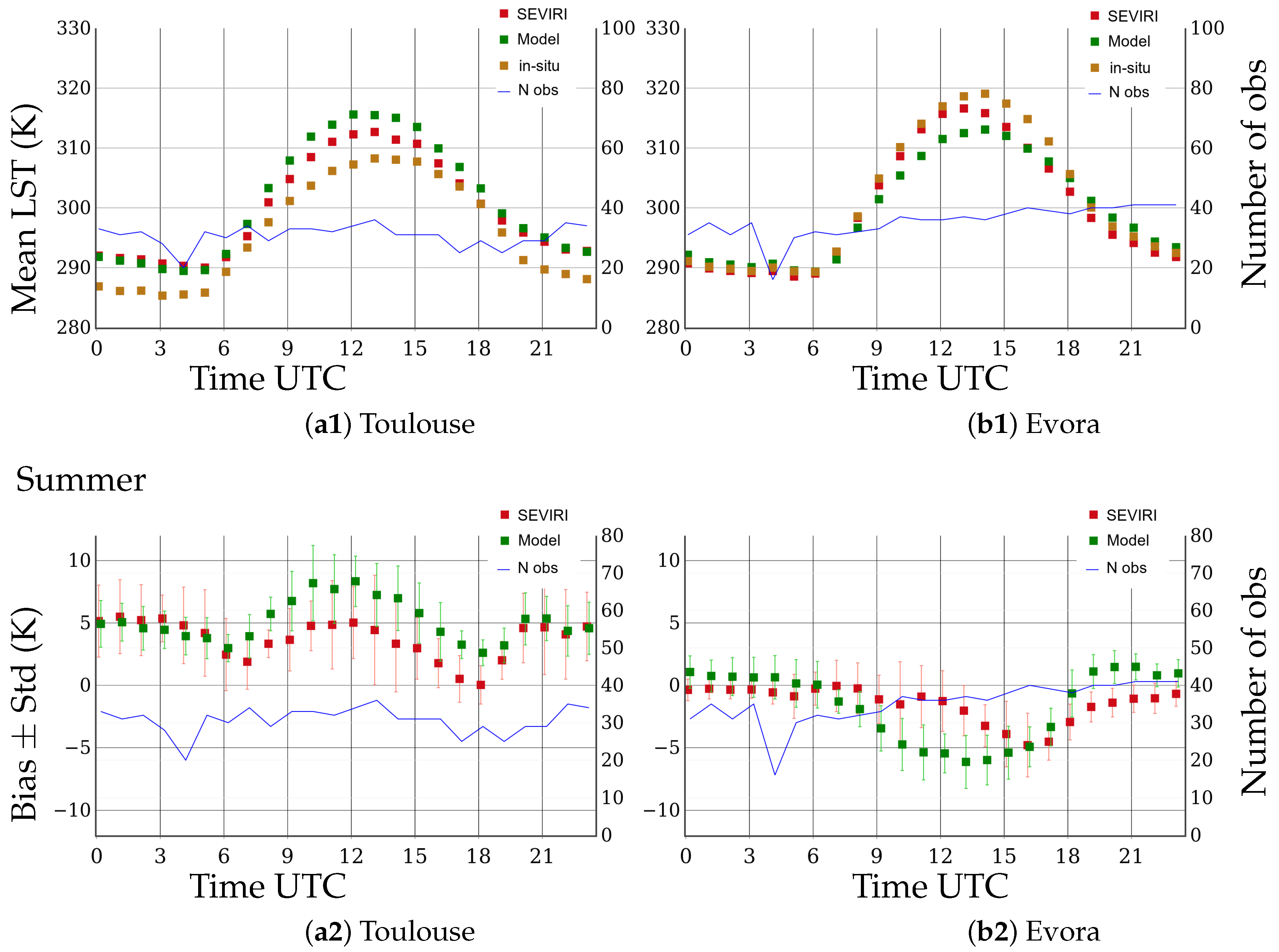
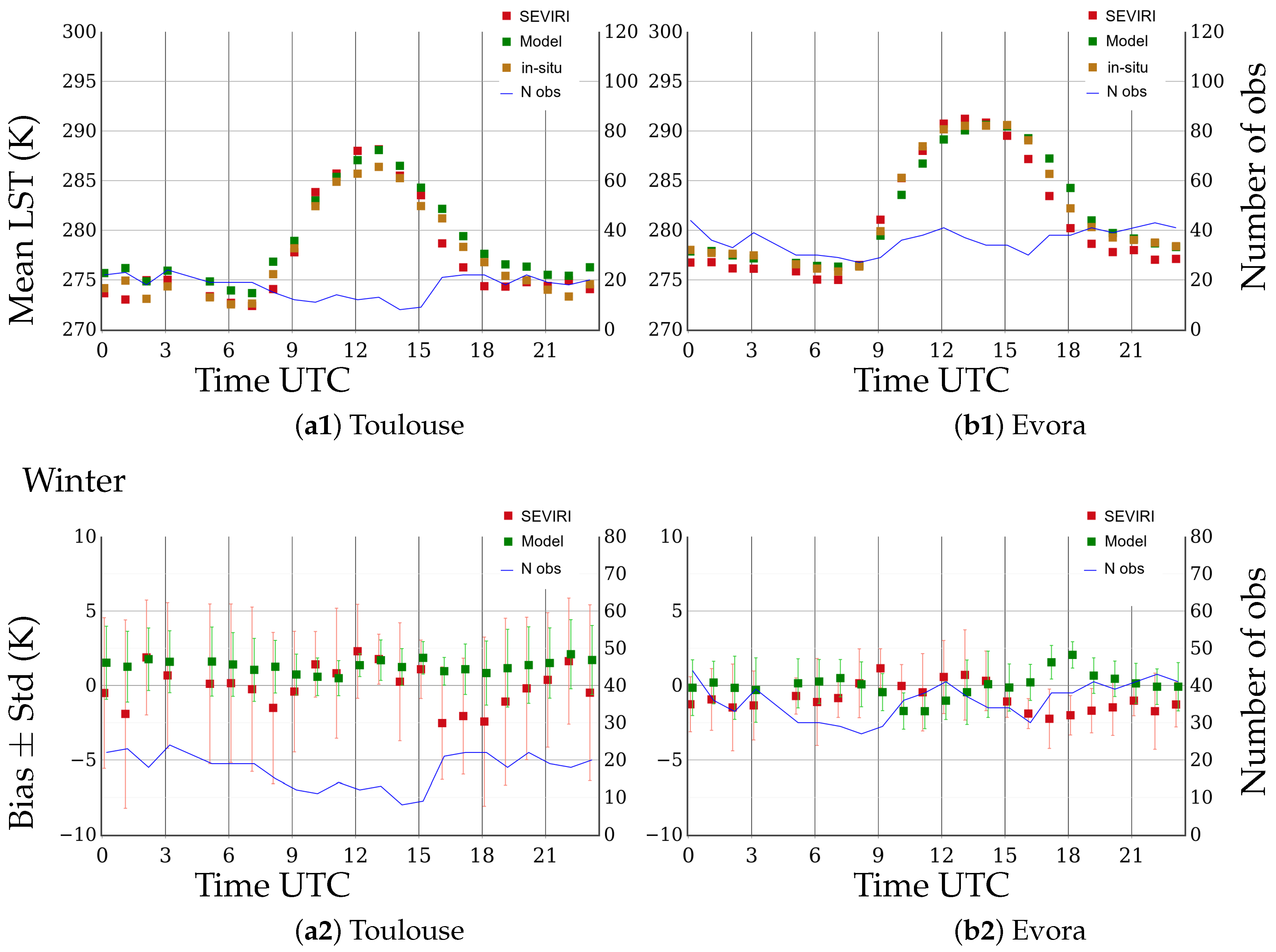
During the summer period (July & August 2018), we found a good agreement between local mean LST from Toulouse station and SEVIRI mean LST. However, model LST overestimates the measured LST. This behavior is noticed during daytime and nighttime as shown in Figure 3(a1). Since Toulouse station is in the suburbs of Toulouse city, it’s worth to mention that AROME-France model includes the Town Energy Balance (TEB) module that takes into account the impact of urban areas on the surface parameters, which might explain the overestimated temperatures by the model. Moreover, the heating effect of the urban areas that might be observed by SEVIRI can contribute to the positive bias of SEVIRI LSTs during daytime as shown in Figure 3(a2). The heating effect can be noticed during nighttime also since urban areas continue to free the heat stored during daytime. An opposite effect is observed for Evora station, which is situated in an area where crops are dominating, but with forested area nearby. In fact, the trees have higher emissivities and have a cooling effect on the LSTs. Figure 3(b1) shows that SEVIRI brings useful information in order to better represent the local LST diurnal variability of Evora station, with a better description of maximum temperature and daytime values. The blue line describes the number of available SEVIRI LST data for every time period.
For Toulouse station, the bias between SEVIRI LSTs and observation is reduced during daytime compared to the bias between model LST and local observation by around 3 K (Figure 3(a2)). The mean difference between model LSTs and observed one exceeds 7 K during daytime (09UTC–13UTC) and remains over 3 K during all the day. In terms of standard deviation, SEVIRI LSTs present in most cases an amplitude of standard deviation varying between 1.5 K and 2.5 K but can exceed 3.5 K in early afternoon. For the comparison between model LSTs and local LSTs, the standard deviation of differences varies in most cases between 1.5 K and 2.5 K with higher amplitudes during early afternoon.
For Evora station, Figure 3(b2) shows that the bias is reduced in most cases with respect to model LST especially during daytime when it can be reduced by up to 4 K. The standard deviation of SEVIRI LSTs with local LSTs difference is also reduced with respect to model LSTs in most cases by up to 0.9 K especially during nighttime.
In Figure 4(a1), the comparison of SEVIRI LSTs with local LSTs from Toulouse station during winter period (January & February 2018) shows a better agreement during daytime than during nighttime. A good agreement is also noticed between local LSTs from Evora station and SEVIRI LSTs which reproduce well its diurnal variability (Figure 4(b1)). In most cases, SEVIRI LST underestimates LST compared to the observation station one. Worth to be mentioned that the SEVIRI observations at 04 UTC were not taken into account in the short cut-off of AROME-France assimilation before July 2018, that is why data from this time period are missing in the winter and spring periods.
Figure 4(a2) shows statistics of difference between SEVIRI LSTs and local LSTs from Toulouse station. During daytime, we find a bias of less than ±2 K with respect to local LSTs in most cases, and a standard deviation from 1.6 K to 4 K. During nighttime, SEVIRI LSTs display larger differences compared to local LST with a bias that can reach −2.5 K. The standard deviation increases also compared to daytime with up to 2 K. The SEVIRI LSTs underestimate the observed LSTs during nighttime in most cases. Contrary to summer period when SEVIRI LSTs presented higher positive bias during daytime and also nighttime, the urban areas have smaller impact on LSTs during winter period. In fact, due to lower illumination conditions, the nearby urban areas contribute much less in heating the surface. Moreover, due to higher cloudiness, possible undetected clouds inside SEVIRI pixels might contribute in the observed negative bias. In Figure 4(b2), the comparison with local LSTs from Evora station presents a bias with an amplitude of less than 2 K and a standard deviation of less than 2.5 K in most cases. Compared to model LSTs, SEVIRI LSTs have, when compared to local LSTs, a smaller bias during daytime and a larger bias during nighttime in most cases.
For Evora station, the number of available clear sky pixels is doubled compared to Toulouse station. It is likely that the higher cloudiness for the latter station explains the higher standard deviation values due to the presence of some undetected clouds. Moreover, depending on which near pixels are clear, the contribution of landscape might be different. In fact, the Toulouse station surrounding landscape is not as homogeneous as for Evora, but is a mixing of urban areas, lake surface and vegetation. Therefore, the contribution of the different landscapes for every SEVIRI pixel is mixed and differs from one pixel to an other.
On other side, we find larger bias amplitudes during the summer period than during the winter period, especially during daytime. For Evora station, SEVIRI LSTs have larger negative bias amplitudes during day time. One possible reason is the shadow/sunlit impact [37]. In fact, the satellite observes the shadow zones covered by the isolated groups of trees in the station area, that are not fully taken into account by the radiometer, which is on a height of only few meters. The shadow/sunlit impact is smaller during daytime in winter period, due to less solar illumination conditions and also lower density of tree leaves, which is in agreement with Figure 4(b2). During nighttime, the underestimation of observed LSTs might be explained by the higher LSEs used for SEVIRI LSTs retrieval during Winter period. In fact, the comparison of Winter and Summer averaged LSEs for Evora area showed higher values during Winter period (not shown).
Table 3 summarizes the statistics of differences of SEVIRI LSTs with local LSTs (SEVIRI LST-Local LST) over the four studied periods for both Toulouse and Evora stations.
Table 3 shows statistics of differences to local observation with SEVIRI LSTs and with model LSTs. During summer period, the bias is reduced by 1.46 K for Toulouse and slightly reduced by 0.12 K for Evora. The standard deviation is slightly increased by 0.63 K for Toulouse but reduced by 1 K for Evora.
During winter period, the bias amplitude between SEVIRI LSTs and local observation decreases by 1.09 K for Toulouse station and increases by 0.89 K for Evora compared to model LSTs. In terms of standard deviation, a higher value is found with SEVIRI LSTs than with model LSTs by 2.88 K for Toulouse station and for Evora by 0.45 K. Worth to mention that the comparison of monthly mean bias for model LSTs compared to local LSTs in Toulouse shows a smaller amplitude of bias during winter period [38].
During Spring and Autumn, we find a reduced bias with SEVIRI LSTs compared to local observation with respect to model LSTs for Toulouse station (by 1.8 K for Spring and 0.92 K for Autumn). However, the bias is increased for Evora station (by 1.29 K for Spring and 0.62 K for Autumn). In the other hand, the standard deviation is increased for both stations.
We evaluated in this first section SEVIRI LSTs compared to local remote sensed LSTs for two observation stations in Toulouse and Evora during four periods from different seasons. The results show a good global agreement especially during summer. SEVIRI LSTs show also better agreement with local LSTs than the model in most cases during daytime. The question then is, what agreement SEVIRI LSTs have with respect to other infrared-sensor LSTs, such as IASI. We discuss this question in the following section.
4. Inter-Comparison of Retrieved LST
In this section, we evaluate how the retrieved LST from various sensors do agree between each other. In AROME-France, LST is retrieved from SEVIRI and IASI sensors before radiance assimilation. This section aims then to quantify the differences between SEVIRI and IASI LSTs in the infrared bands.
The inter-comparisons are restricted to IASI LSTs and SEVIRI LSTs in clear sky conditions.
4.1. Spatial and Temporal Colocalization
To compare SEVIRI and IASI LSTs, we used the retrievals produced hourly over the AROME-France domain. We considered the SEVIRI observations taken on sharp hours. The IASI observations are taken within an elapse period of less than 30 min from SEVIRI observations. In terms of spatial colocalization, SEVIRI LST is a mean value of the clear pixels available within 4.5 km from the IASI center of pixel, so SEVIRI pixels not fully included in IASI pixels are excluded from comparison. We decided not to take into account the SEVIRI pixels size variability since its impact was small on the comparison. In fact, the size of SEVIRI pixels slightly changes over the AROME-France domain [39]: The E-W component of the SEVIRI pixel ground resolution does not vary over the AROME-France domain while the N-S component varies from 5 km to 6 km in most cases, reaching 8 km in the north-eastern part of the domain. On the other hand, an orography threshold of 400 m has been applied for SEVIRI and IASI data, rejecting observations in mountainous areas.
4.2. Results of Comparison with IASI
SEVIRI and IASI instruments observe the AROME-France domain with different viewing angles. Knowing the dependence of vegetation and topography impact with respect to the viewing angle in LST estimation by daytime for different sensors [40], we decided to evaluate the differences between IASI LST and SEVIRI LST separately for nighttime and for daytime when the viewing angle has more impact [41]. As an example, the correlation between the scan position of IASI instrument and the difference between the two sensor’s LSTs is around zero during nighttime for all seasons, however, it rises during daytime to around 0.3 for summer period and 0.4 for winter period.
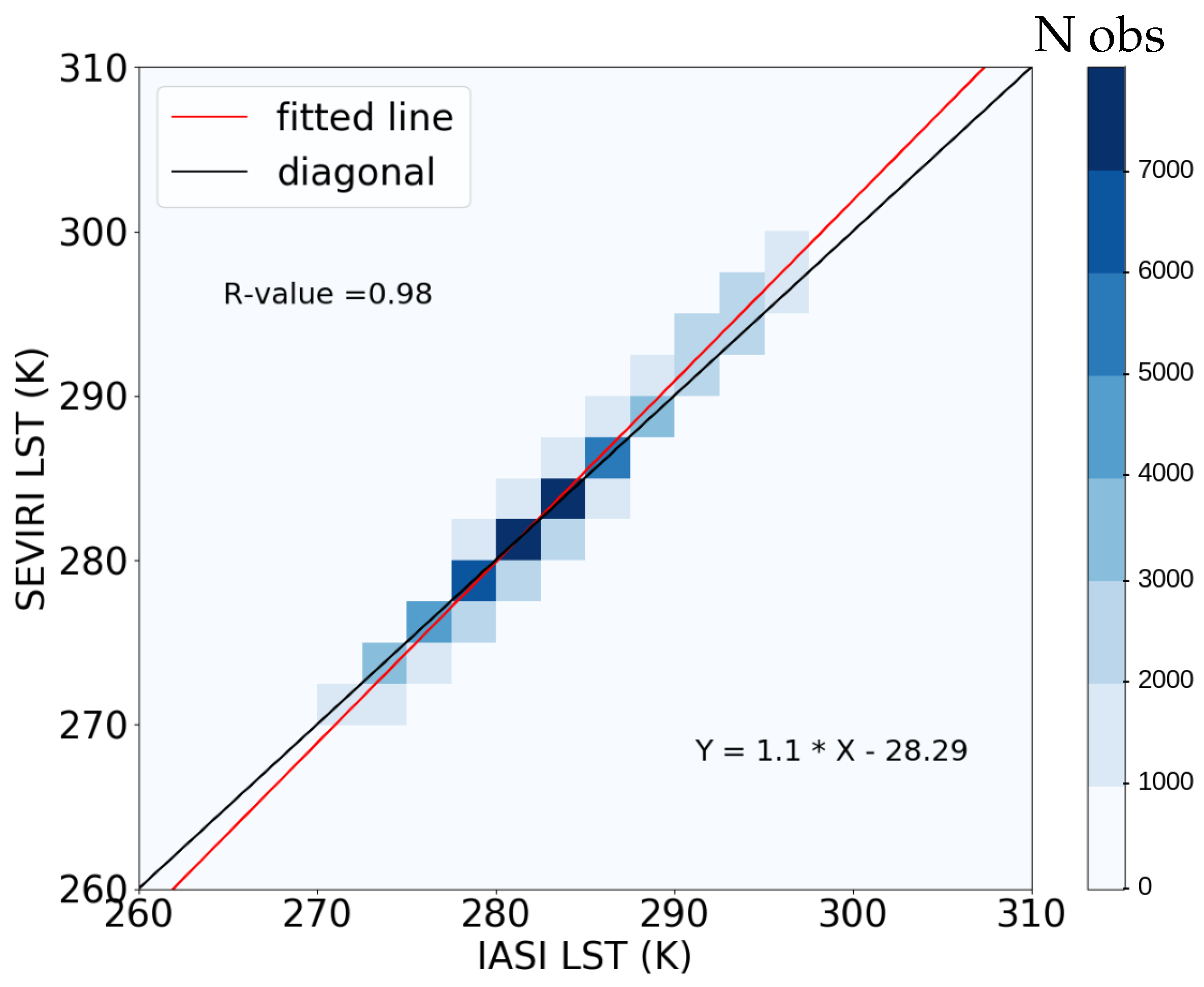
Figure 5 shows a 2D histogram of IASI and SEVIRI LSTs for October and November 2018 which highlights a strong positive correlation ( Pearson correlation coefficient = 0.98). SEVIRI LSTs are warmer for maxima and colder for minima which gives a higher amplitude for diurnal cycle than for IASI as explained later.
A better agreement between SEVIRI and IASI LSTs is also found for colder temperatures which correspond to nighttime temperatures (Figure 5).
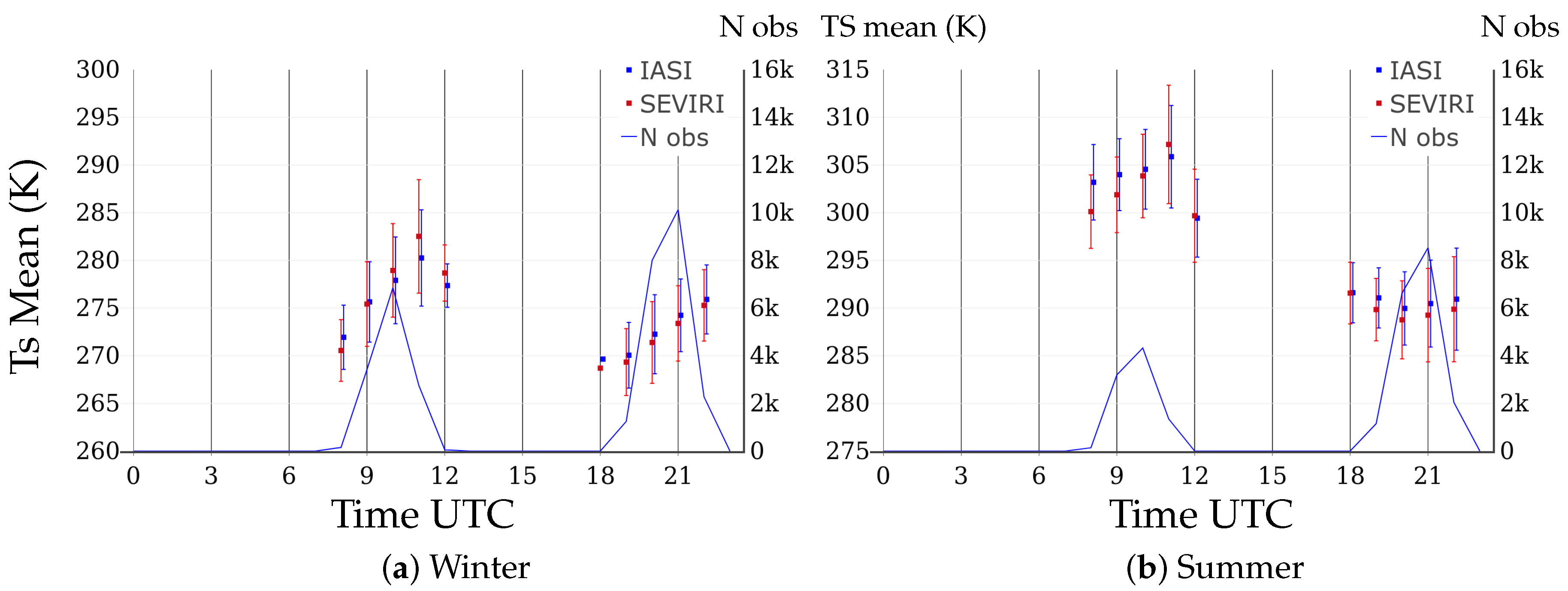
Figure 6 shows a global agreement between the diurnal cycles of SEVIRI and IASI LSTs, especially during nighttime when differences in mean LST remain less than 1 K. SEVIRI LST mean values are calculated taking into account the spatial and temporal co-localization with IASI data. The polar orbit of Metop satellites carrying the IASI sensor and their coverage from the northern colder part to the southern warmer part of the domain contributes to the increase of the LST mean values as noticed during nighttime hours for the winter diurnal cycle. This impact is not observed for the summer diurnal cycle because of the longer daytime. Note that the lack of data during daytime for summer period might be explained by the reduced transmittance due to the increase in water vapor content in the atmosphere which impacts the LST retrieval [42].
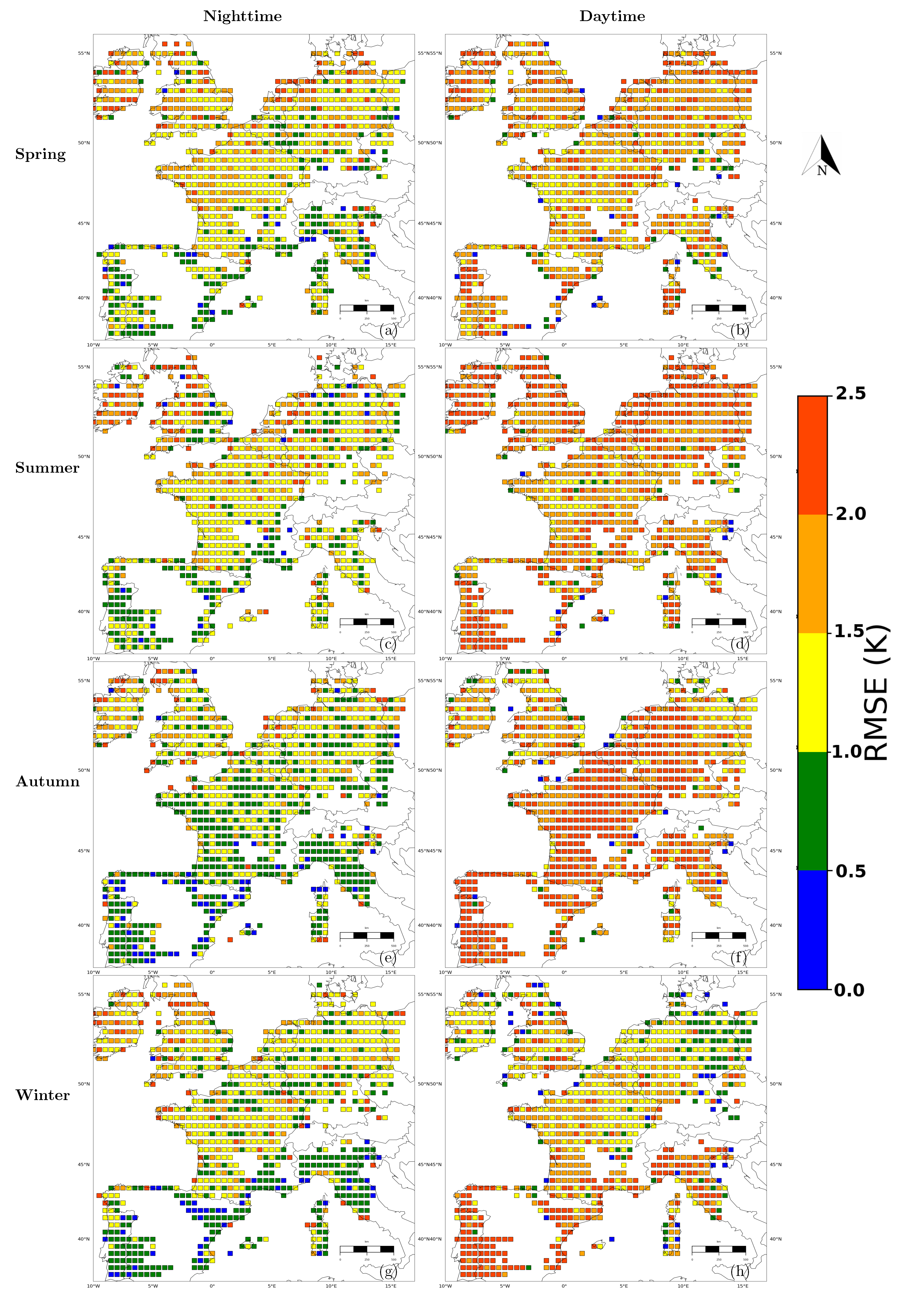
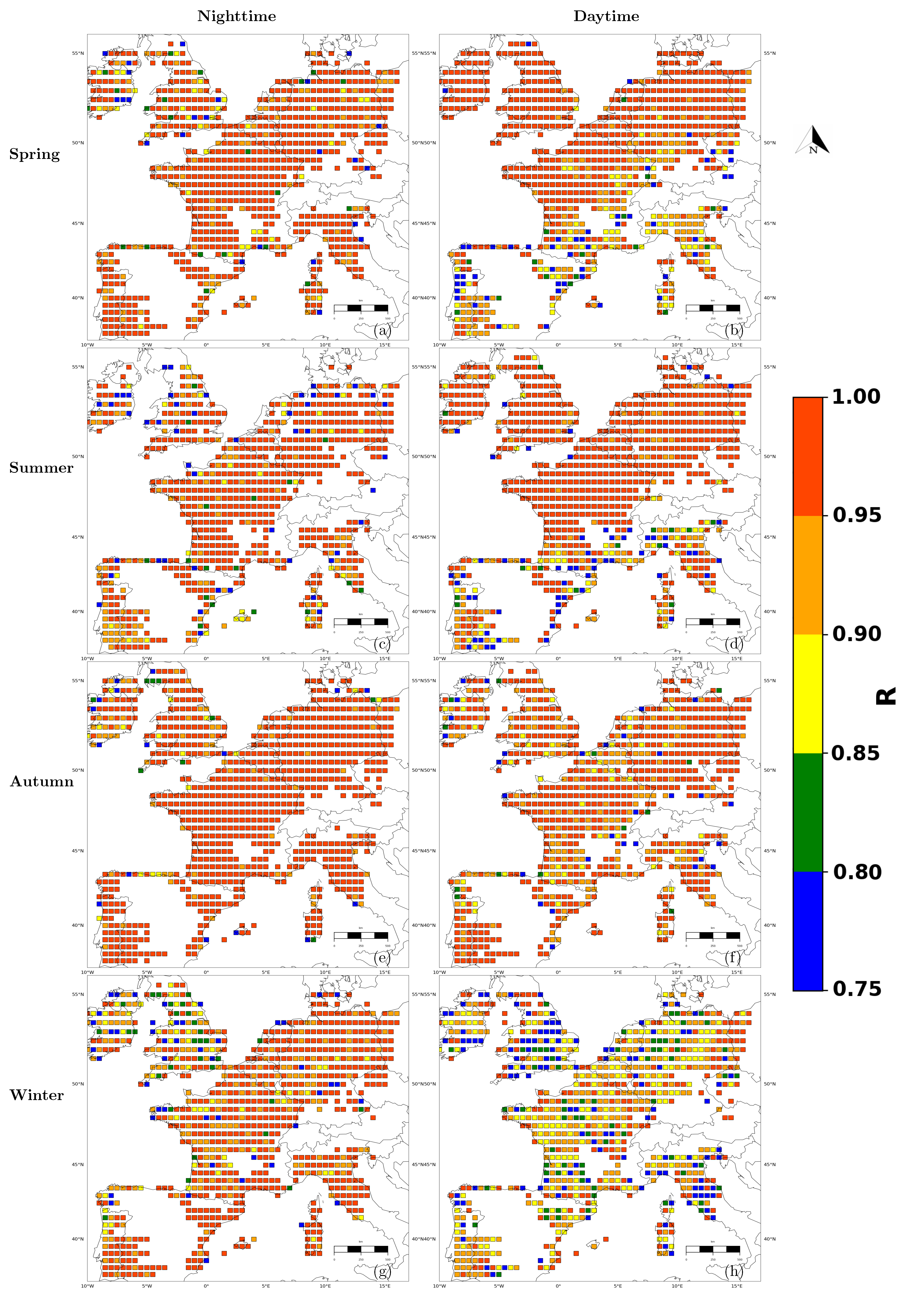
In order to evaluate the spatial variability of the differences, we plotted the root mean square errors and the correlation coefficients for each period between IASI and SEVIRI LSTs averaged on a 0.5× 0.5 grid as shown respectively in Figure 7 and Figure 8.
Figure 7 and Figure 8 show respectively the IASI LSTs and SEVIRI LSTs differences statistics in terms of RMSE and correlation coefficients during nighttime (a, c, e, g) and daytime (b, d, f, h) for the different periods. The nighttime comparisons show comparable statistics in terms of RMSE for the different seasons. The higher values of RMSE can be noticed mainly over the northern parts of the domain. This might be due to smaller mean differences over the southern part of the domain especially the Iberian peninsula (not shown). Moreover, The cross-correlation of IASI and SEVIRI LSTs described in Figure 8 shows a globally homogeneous correlation dispersion with correlation coefficients higher than 0.9 for Summer, Spring and Winter and higher than 0.95 in most cases for Autumn. On the other hand, we can notice high values of RMSE and also low correlation coefficients on some coastal boxes, which can result from the different sizes of IASI and SEVIRI pixels and then different contributions from sea surface in the sensors coastal pixels. The summer time comparisons use less data over the northern part of the domain during nighttime, due to the polar orbit of Metop satellites which covers that area twice during daytime at around 09–10 UTC and 19–20 UTC.
The daytime comparisons point out higher values of RMSE compared to nighttime. The highest values of RMSE are noticed for Summer and Autumn periods. These high RMSE values are mainly explained by higher mean differences during Summer period and higher standard deviation values during Autumn as shown in Table 4. Contrary to nighttime comparisons, the southern part of the domain, mainly the Iberian peninsula and north of Italy shows high RMSE values in addition to smaller correlation coefficients of less than 0.9. These higher differences between IASI LSTs and SEVIRI LSTs might be due to proximity from mountainous areas where shadow/sunlit effect can have more impact.
Table 4 summarizes the statistics of difference between IASI LSTs and SEVIRI LSTs averaged over the full domain during nighttime and daytime for Spring, Summer, Autumn and Winter comparison periods. Table 4 shows a better agreement between IASI LSTs and SEVIRI LSTs by nighttime than by daytime. In fact, the nighttime comparisons in different periods give smaller absolute values of mean difference in most cases (except for spring when bias is increased from 0.77 K during daytime to 1.05 K during nighttime). In the case of spring and summer periods, the mean difference remains positive during both nighttime and daytime. However, in autumn and winter periods, the bias is positive for nighttime comparisons and negative for daytime case. Comparing the absolute values of bias between nighttime and daytime, we find a difference of about 0.1 K in winter period (−0.94 K during daytime and 0.83 K during nighttime) and about 0.3 K in autumn period (−1.04 K during daytime and 0.70 K during nighttime).
Several effects might explain the difference in terms of bias between Spring and Summer periods compared to Autumn and Winter periods while it remains difficult to quantify their respective impact. On one hand, the comparison of surface emissivities used for IASI and SEVIRI LSTs retrieval shows a varying mean of difference according to the period (not shown). The higher differences were noticed in Summer and Spring periods with a negative mean difference (IASI LSEs–SEVIRI LSEs). This might add a positive bias to the LSTs comparison compared to Autumn and Winter periods. On the other hand, the difference in terms of solar illumination conditions and the impact of shadow/sunlit effect, due to the different viewing angles of IASI (on-board polar satellites) and SEVIRI (on-board geostationary satellite) might contribute also in the different behavior of mean differences. Furthermore, higher cloudiness in Autumn and Winter periods might also contribute to explain the negative mean differences. In fact, two different cloud detection algorithms are used for IASI and SEVIRI. While IASI pixels are larger than SEVIRI ones, the impact of undetected clouds can be higher on IASI LSTs than on SEVIRI LSTs leading to colder IASI LSTs. This effect can also occur during nighttime and is in agreement with nighttime statistics which show smaller mean difference values during Autumn and Winter periods.
In terms of standard deviation of differences, smaller values are obtained during nighttime than during daytime comparisons for all periods. The differences between daytime and nighttime standard deviation values remain less than 1 K in all periods of comparison. During nighttime, the standard deviation values remain very close between the different periods of comparison and varies within 0.06 K. During daytime, the standard deviations vary within 0.1 K for the different period except for Autumn period when it reaches 1.93 K.
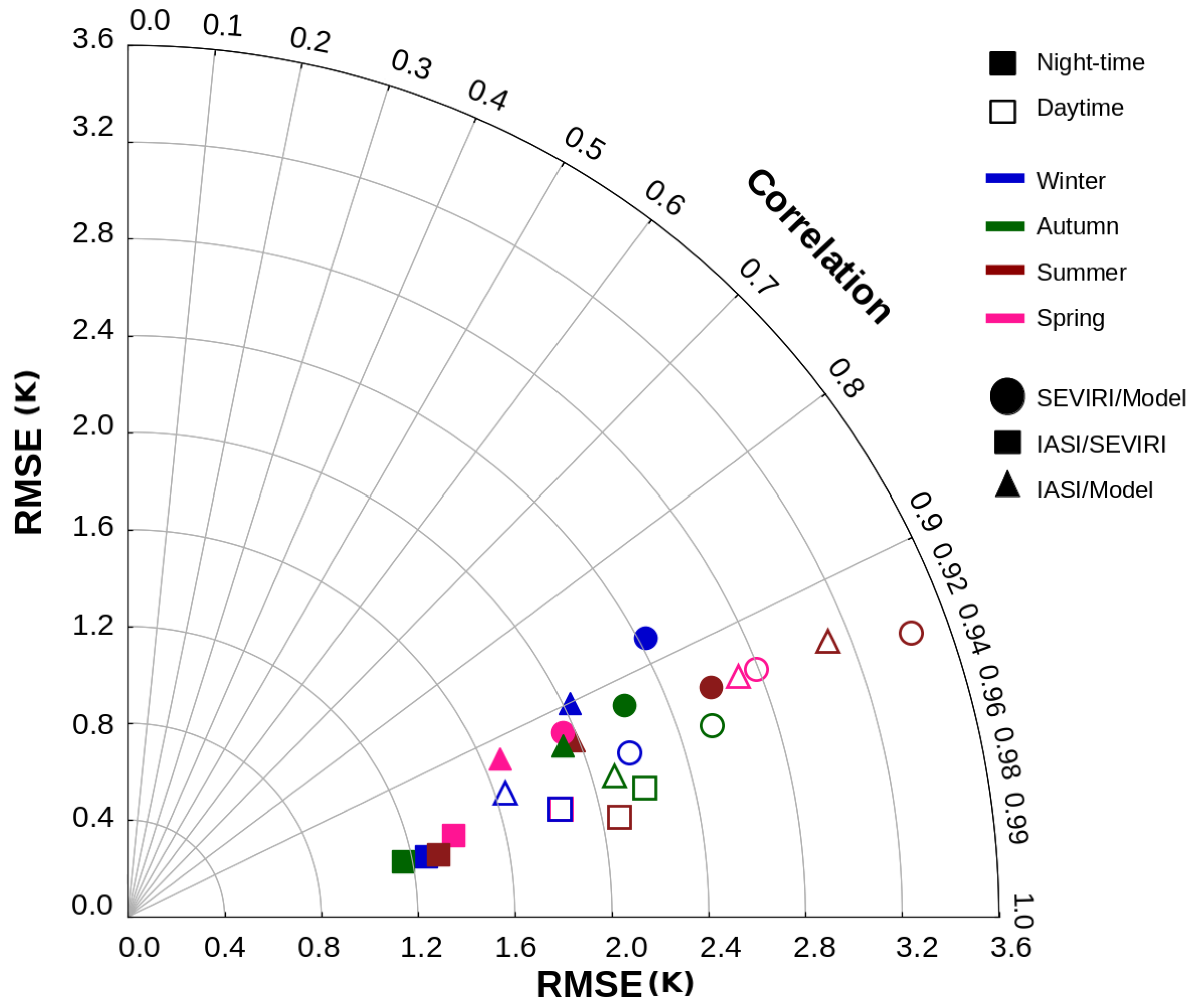
Figure 9 shows a Taylor diagram of the statistics of differences between IASI LSTs and SEVIRI LSTs during daytime and nighttime for the four periods of comparisons. The Taylor diagram takes into account the correlation coefficient between both LSTs and the root mean square errors (represented by squares). The diagram also presents the statistics of differences of SEVIRI LSTs with model LSTs (represented by circles) and the statistics of differences of IASI LSTs with model LSTs (represented by triangles). We can then notice that, on one hand, we have less differences between SEVIRI LSTs and IASI LSTs than between each sensor LSTs and the colocalized model LSTs and on the other hand, the correlation is higher between both infrared LSTs than between infrared LSTs and model LSTs. Moreover, while comparing the model LSTs against the two sensors LSTs, we can notice smaller differences between the model LSTs and IASI LSTs than between the model LSTs and SEVIRI LSTs.
In addition, it could be beneficial to consider the differences against local LSTs for both sensors. As a perspective, the statistics of difference for both sensors LSTs against local LSTs could be compared to the statistics of the differences between both sensors and of each sensor against the model.
Figure 9 also shows that, during daytime for autumn and winter periods, IASI LSTs agree better with model LSTs than with SEVIRI LSTs. This can be related to a higher cloudiness and a lower transmittance which might reduce the number of clear sky SEVIRI pixels inside the IASI pixel and consequently reduce its representativity. The differences might be due also to the different atlases defining the LSEs used for the two sensors retrievals. In fact, the two atlases are calculated with different approaches. They define monthly mean values of LSEs for every spectral band, and then might agree between each other in one month more than the other. As a perspective, it’s worth to evaluate the impact of considering a unique infrared surface emissivity atlas for both sensors.
The inter-comparison of the two infrared sensors LSTs during four different periods shows a high correlation and a good agreement especially during nighttime. We noticed also that the two sensors’s LSTs show better agreement between each other than with model LSTs. A second question then arises, what is the impact of the different LST in the simulation of IASI and SEVIRI brightness temperatures. We answer to this question in the following section.
5. Impact of LST in RTTOV Simulations
In this section, we evaluate the impact of using one sensor LST in order to simulate the brightness temperatures of the other. For this, we have run two series of simulations using the RTTOV model. The first simulates IASI brightness temperatures while the second simulates the SEVIRI ones.
5.1. Principle of the Experiment
In order to simulate brightness temperatures with RTTOV, a background information i.e., vertical atmospheric profiles of temperature and humidity and a surface temperature is needed. Therefore, more than 21,000 vertical profiles have been extracted over land (See Appendix A.1) from the AROME-France model representing different soil occupations and different areas of the AROME-France model domain (around 9000 profiles for daytime conditions and more than 12,000 profiles for nighttime conditions). Worth to mention that RTTOV model includes a module to take into account the errors resulting from the angle difference between the viewing angle of the sensor and the vertical profile of the model. For the land surface temperature, we defined three different values: IASI LST, SEVIRI LST and the one forecasted by the model. Moreover, for every profile simulation, the same emissivity value as the one used for the LST operational retrieval has been also used for the three simulations. Finally, as in the previous section, we considered clear sky retrievals only with an orography threshold of 400 m.
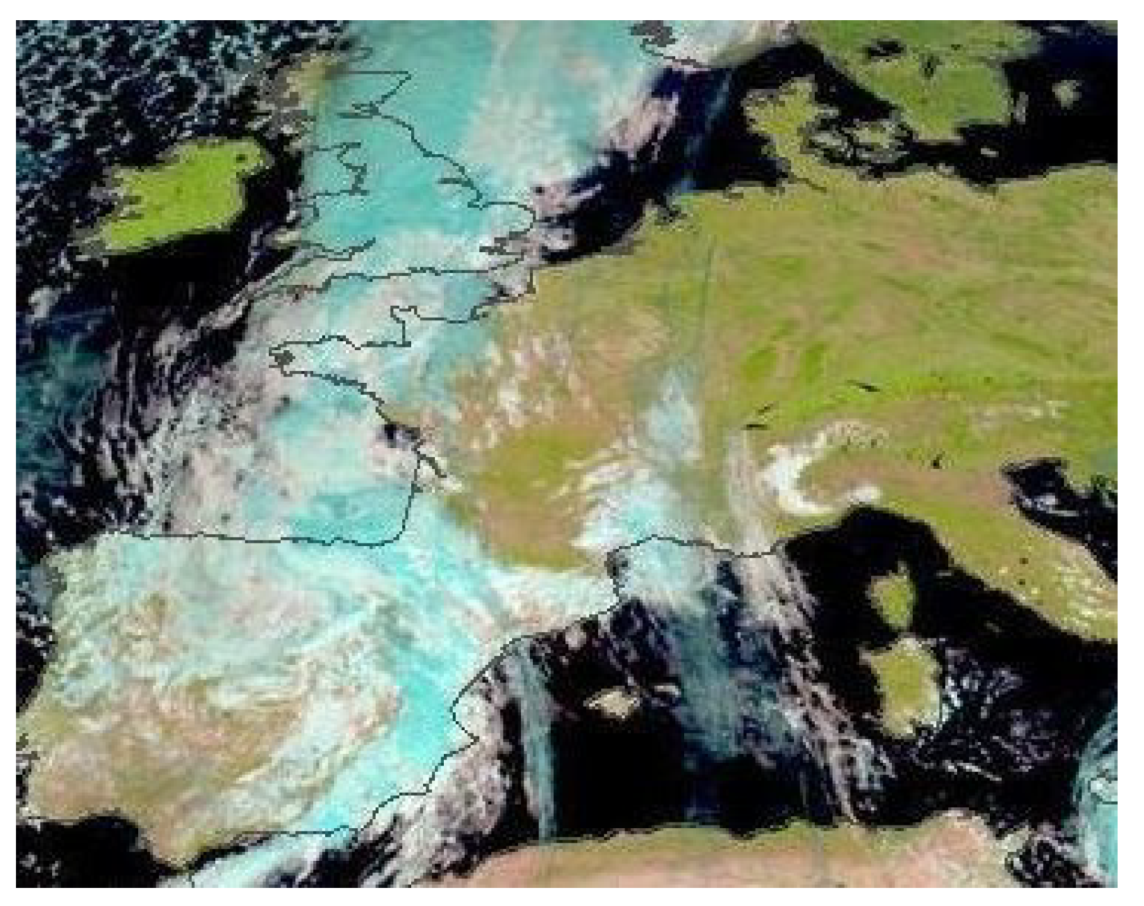
The two series of simulations, were run over 32 days, 8 from each season (The days of 07th, 14th, 21st and 28th of January, February, April, May, July, August, October and November 2018). As an example, Figure 10 describes the cloud cover for the simulation of the October 14th 2018. Profiles have not been extracted for simulation in regions where clouds are present.
5.2. IASI Simulations
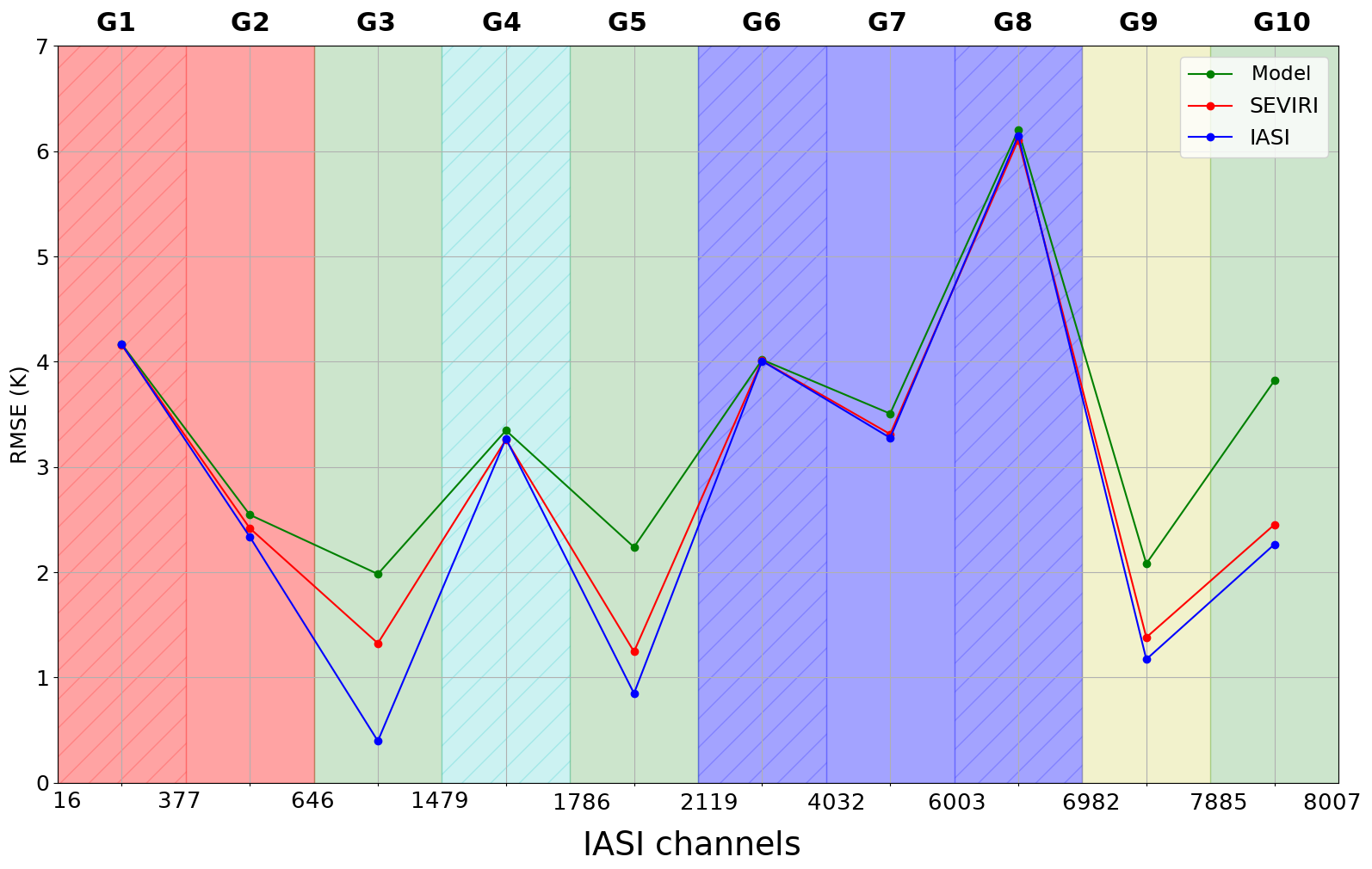
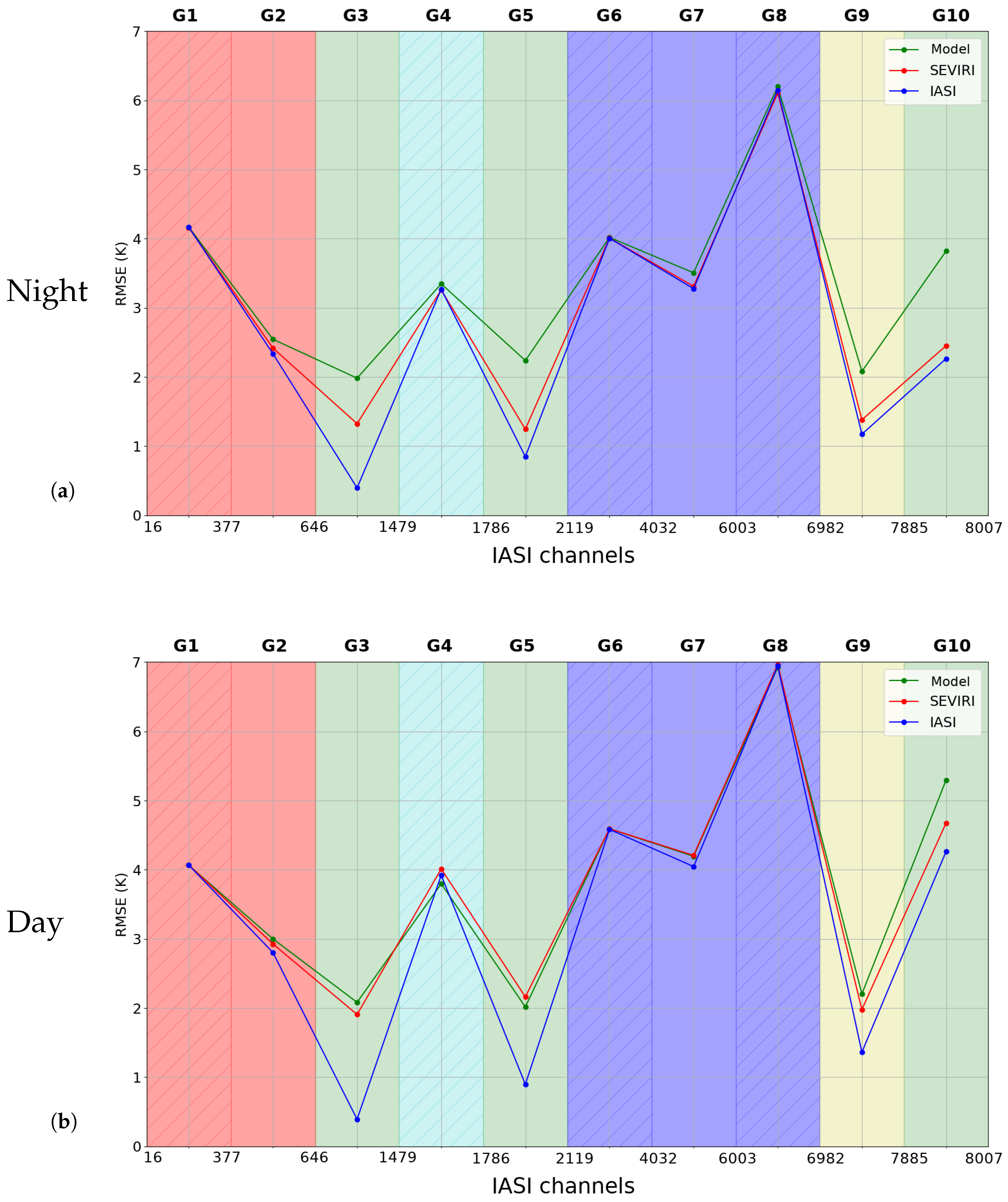
The first series of RTTOV run simulates a set of 314 IASI channels monitored at Météo-France [43]. The simulated brightness temperatures were then compared to the observed ones. As IASI channels have different sensitivities to surface, they have been grouped into 10 families, in the temperature, surface, ozone, water vapor and solar sensitive wave-lengths (See Appendix A.2). In the following paragraph, we present the root mean square errors of the brightness temperatures observed by IASI minus the simulated ones using each of the three surface temperatures.
Figure 11a,b describe the statistics of observation departure (obs-simulations) according to the LST used as an input of RTTOV simulation during nighttime and during daytime.
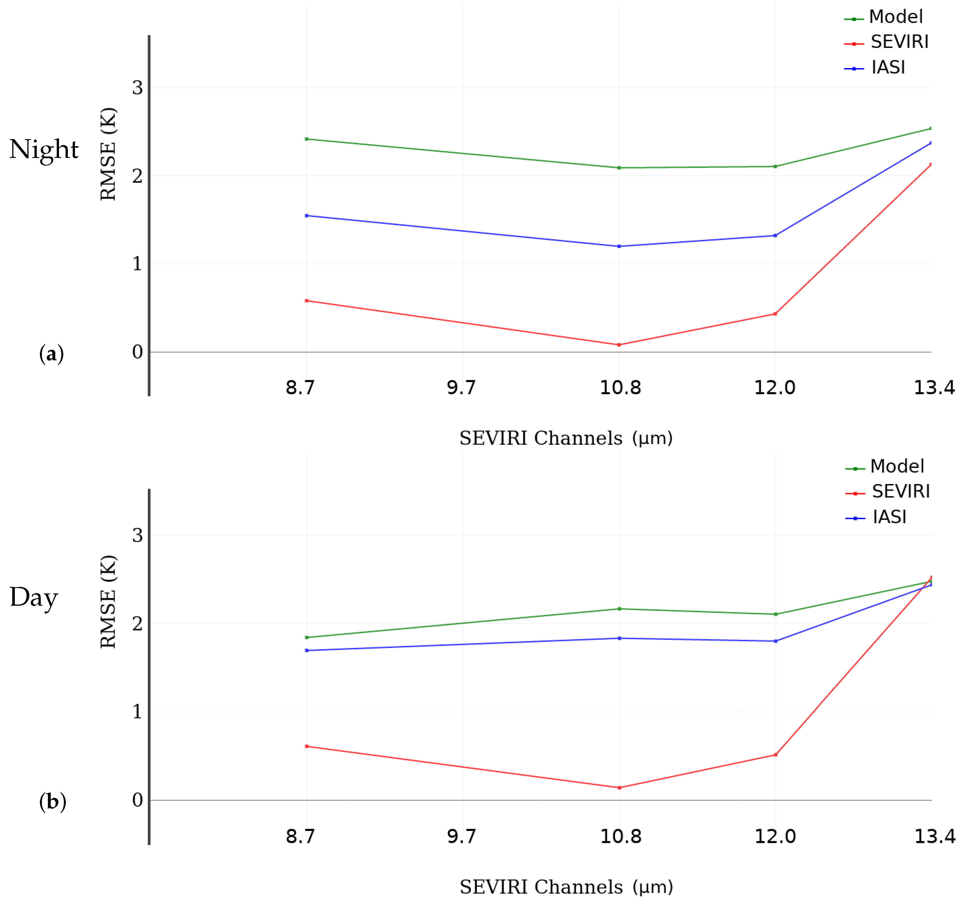
Figure 11a shows different impacts of using each value of LST for nighttime simulations with higher impact on surface sensitive channels. The best simulations are obtained using IASI LST. SEVIRI LST slightly increases the RMSE compared to IASI LST but gives for all channels better simulations than model LST. As an example, the simulation of first set of surface sensitive channels (G3) gives a RMSE of 0.4 K using IASI LST, 1.32 K using SEVIRI LST and 1.98 K using model LST. The second set of surface sensitive channels (G5) gives a RMSE of 0.85 K using IASI LST, 1.24 K using SEVIRI LST and 2.24 K using model LST. The additional surface sensitive channels (G10) give higher RMSE of 2.26 K with IASI LST, 2.45 K with SEVIRI LST and 3.82 K with model LST. For solar channels (G9), SEVIRI LST increases the RMSE by 0.21 K compared to IASI LST while model LST increases the RMSE by 0.91 K. For the temperature, ozone and water vapor channels, the differences in terms of RMSE between using IASI LST and SEVIRI LST are of less than 0.08 K, while it can exceed 0.2 K between using IASI LST and model LST.
Figure 11b shows the daytime simulations. As seen for the nighttime case, IASI LST allows the best simulations. However, we notice a larger degradation of SEVIRI LST which increases the RMSE compared to IASI LST more than for the nighttime simulation. Moreover, during daytime, SEVIRI LST gives simulations that are in most of cases better than model LST simulations but at the same time closer to model LST simulations than to IASI LST simulations. As an example, for surface sensitive channels (G3), IASI LST gives a brightness temperature RMSE of 0.39 K while SEVIRI LST gives a RMSE of 1.91 K and model LST a RMSE of 2.08 K. Finally, a slightly increased RMSE with SEVIRI LST than with model LST is noticed for ozone sensitive channels (RMSE increased by 0.22 K) and the surface channels G5 (RMSE increased by 0.15 K). This was not the case for nighttime simulations when SEVIRI LST provides better simulations than model LST in all the cases.
Figure 11a,b show the averaged statistics over the four periods of study, but a further look into each season (not shown) has revealed a seasonal variability. In fact, during nighttime, the impact of the use of SEVIRI LST on the IASI brightness temperature simulation is smaller for summer and spring periods. Compared to model LST, SEVIRI LST always provides better simulations. However, during daytime, model LST provides better simulations for surface sensitive channels than SEVIRI LSTs during winter and autumn. This meets the results of sensors inter-comparison shown on Figure 9 where IASI LSTs present better agreement with model LSTs than with SEVIRI LSTs during daytime, for winter and autumn periods.
5.3. SEVIRI Simulations
The second series of RTTOV run simulated the SEVIRI brightness temperatures while using different values of LSTs and were then compared to SEVIRI observations.
Figure 12a shows the root mean square errors of SEVIRI simulated brightness temperatures with respect to the observations during nighttime with different LST values. SEVIRI LST gives the best simulation. IASI LST increases the RMSE compared to SEVIRI LST but gives better simulations than with model LST. As an example, for channel 6 (10.8 m) used for the operational SEVIRI LST retrieval, SEVIRI LST gives a RMSE of 0.08 K while IASI LST gives a RMSE of 1.24 K and model LST a RMSE of 2.19 K.
For daytime simulations, Figure 12b shows higher impact of using different values of LST especially for surface sensitive channel 6 (10.8 m) where the use of IASI LST increased the RMSE by 1.73 K and the use of model LST increased the LST by 2.23 K with respect to the use of SEVIRI LST.
In terms of seasonal variability, less differences were noticed for SEVIRI simulations compared to IASI simulations not shown. In fact, for both nighttime and daytime simulations, the use of IASI LST increased the RMSE compared to SEVIRI LST but gave smaller RMSE than the model for the four seasons. Finally, for daytime simulations, a higher impact of using IASI LST was noticed during winter and autumn seasons as seen for the IASI simulation case. The simulation of IASI and SEVIRI infrared sensor brightness temperatures with RTTOV model using different values of LSTs showed that the best simulations were obtained with the simulated sensor’s retrieved LST, while the other sensor’s retrieved LST increased slightly the RMSE but gave in most cases better simulations than model LST, especially during nighttime.
This section showed encouraging results of IASI and SEVIRI channels simulations. For every sensor simulation, we obtained better simulations while using the second sensor LSTs than with the model LSTs (in most cases for IASI and all cases for SEVIRI). This leads to think that considering an alternative LST that is based on both model LST and remotely sensed LST might improve the model equivalents of the observations and consequently the sensor channels assimilation.
6. Conclusions and Perspectives
The current study consists in a preliminary step in order to assimilate LST in the surface analysis of Météo-France NWP models. We focus on the two infrared sensors SEVIRI and IASI LSTs and the model LSTs in order to study the agreement between them and evaluate their impact on the radiative transfer simulation. The first part of this work provided a comparison of SEVIRI retrieved LSTs against local observations available from Toulouse Meteopole and Evora stations. The comparisons are done between in-situ observations and the mean value of SEVIRI pixels within a radius of 4.5 km. A good agreement is found in terms of diurnal variability of LSTs. The differences vary as a function of season with a better agreement during summer for Toulouse station and a better agreement during winter for Evora. To explain these results, we need to take into account the different environments of the two observation stations. For Toulouse station, a comparison between different SEVIRI pixels around the station shows a better agreement of LSTs with pixels observing a more representative terrain of the station compared to the terrain observed by the radiometer. The positive bias during summer might be explained by the proximate urban area heating effect. This impact is reduced during winter period which agrees with the comparison results. For Evora station, the tree shadow could explain the larger negative biases observed during summer. However, during winter period the lower solar illumination and the loss of leaves can reduce the shadowed areas compared to summer period, which might explain the smaller bias during daytime. This comparison also included forecasted LSTs from the AROME-France model. For both stations, SEVIRI LSTs agree better with respect to local observations than with model LSTs during spring and summer. However, during winter and autumn, SEVIRI LSTs show higher variability. The comparison of model daytime LSTs between Toulouse and Evora stations showed that the model overestimated LSTs for Toulouse station and underestimated LSTs for Evora station. This different behavior might be explained by the different land covers in the model which consist of a proximate urban area for Toulouse station and disperse trees with a proximate forest for Evora station.
In a second part, we presented a comparison between SEVIRI and IASI retrieved LSTs. Due to a higher impact of viewing angle during daytime on retrieved LSTs, we presented the results separately for daytime and nighttime. A good global agreement between LSTs from both sensors was found. The comparison of diurnal variability of both sensors for temporally colocalized LSTs showed a good agreement especially during nighttime. Furthermore, we have noticed smaller RMSE of differences of IASI LSTs minus SEVIRI LSTs during nighttime than during daytime for the four periods of study. During daytime, higher values of RMSE were found during summer and autumn periods with higher mean of differences during summer period and higher standard deviation during autumn. The comparison of LSTs mean difference shows positive values during summer and spring periods contrary to autumn and winter periods which gave negative values. Different conditions might contribute to such behavior such as the higher cloudiness during autumn and winter periods which might reduce the representativity of SEVIRI pixels compared to IASI ones. Moreover, the different solar illumination conditions and the different surface emissivities for IASI and SEVIRI retrievals can also contribute to explain the obtained mean differences of LSTs. The evaluation of IASI LSTs differences compared to SEVIRI LSTs gave biases and standard deviations with values less than 1.5 K in most cases. In terms of bias, IASI presented a positive bias during nighttime from around 0.7 K during autumn period to around 1 K during spring period with a strong positive correlation. The spatial distribution of cross-correlation between IASI LSTs and SEVIRI LSTs is well homogeneous and gave a Pearson coefficient higher than 0.95 in most cases. However, during daytime, the cross-correlation between IASI LSTs and SEVIRI LSTs gave smaller correlation coefficients during Winter, varying between 0.75 and 0.9. The correlation coefficients are higher than 0.95 in most cases during Summer and Spring for the northern part of the domain but smaller values where obtained in the southern part, which might be due to proximity to mountainous areas that increases the sunlit/shadow impact. In terms of bias, IASI presented negative values during autumn and winter. The bias during daytime varied from −1 K in autumn to around +1.2 K in summer. Then, we have evaluated the difference between both sensors LSTs against the model forecasted LSTs and the SEVIRI and IASI LSTs do better agree between each other than with model LSTs. As a perspective, a further step can consist in comparing the IASI LSTs against the in-situ LSTs in order to better understand the differences between the sensors.
In the third part we studied the impact of using the LSTs of one infrared sensor in order to simulate the brightness temperatures of the other. The IASI brightness temperature simulations showed better statistics with observations in terms of RMSE with IASI LSTs. In agreement with the results of the second part, the use of SEVIRI LSTs increased the RMSE slightly during nighttime but gave better simulations than with model LSTs for all the simulated channels. During daytime, the use of SEVIRI LSTs gave worse results but in most cases smaller RMSE than with model LSTs. Concerning the SEVIRI brightness temperature simulations, the best statistics against observations were obtained with SEVIRI LSTs. The use of IASI LSTs increased the RMSE but gave better simulations than with model LSTs for both nighttime and daytime simulations. In terms of seasonal variability, a better agreement between simulated brightness temperatures using retrieved LSTs has been found during spring and summer than during autumn and winter.
These results are encouraging to use retrieved LSTs for further applications. The better impact of using LSTs from different sensors than using model LSTs for the brightness temperature simulations makes us expect a potential positive impact of the use of satellite retrieved LSTs in the surface analysis. Further work will consist in evaluating the impact of using a single retrieved LST for the assimilation of the infrared sensors instead of using a retrieved LST for every infrared sensor. This study will be extended to microwave sensors and the retrieval of surface emissivity instead of LST will be considered, as the microwave emissivity has a much larger variability in the microwave range than in the infrared range. The retrieved LSTs will then be used to initialize the soil temperature, in the current surface analysis system. The current system uses 2-m air temperature to analyze the soil temperatures and the impact of using satellite retrieved LSTs will be assessed. Both surface and deep soil temperatures will be updated using retrieved LSTs in order to propagate the impact from an assimilation cycle to the next. Then the impact of the new surface analysis will be evaluated on forecasts. More realistic surface state is expected to improve the model forecasted low layer variables and the brightness temperature simulation in the atmospheric analysis.
Author Contributions
Conceptualization, N.F., V.G., C.B.; methodology, N.F., V.G., C.B. and M.Z.S.; software, N.F., V.G., C.B. and M.Z.S.; validation, N.F., V.G., C.B. and M.Z.S.; formal analysis, N.F., V.G., C.B. and M.Z.S.; investigation, N.F., V.G., C.B. and M.Z.S.; resources, N.F., V.G., C.B. and M.Z.S.; data curation, N.F., V.G., C.B. and M.Z.S.; writing—original draft preparation, M.Z.S.; writing—review and editing, N.F., V.G. and C.B.; visualization, M.Z.S.; supervision, N.F., V.G., C.B.; project administration, N.F. and V.G.; funding acquisition, N.F.
Funding
The PhD of Mohamed Zied Sassi is funded by Météo-France and Région Occitanie.
Acknowledgments
Thanks to KIT for the Evora station local data and to Météopole-Flux for Toulouse station data.
Conflicts of Interest
The authors declare no conflict of interest.
Abbreviations
The following abbreviations are used in this manuscript:
| LST | Land Surface Temperature |
| T2m | 2-m air temperature |
| RH2m | 2-m relative humidity |
| NWP | Numerical Weather Prediction |
| UTC | Universal Time Coordinated |
| MSG | Meteosat Second Generation |
| KIT | Karlsruhe Institute of Technology |
| IASI | Infrared Atmospheric Sounding Interferometer |
| SEVIRI | Spinning Enhanced Visible and Infrared Imager |
| AROME | Applications de la Recherche à l’Opérationnel à Méso-Echelle |
| CNRM | Centre National de Recherches Météorologiques |
| MSG | Meteosat Second Generation |
| RTTOV | Radiative Transfer for TOVS |
| TOVS | TIROS Operational Vertical Sounder |
Appendix A
Appendix A.1.

Table A1.
The number of AROME-France vertical profiles used in RTTOV simulations.
| Season | Number of Vertical Profiles |
|---|---|
| Spring | 4674 |
| Summer | 4030 |
| Autumn | 5970 |
| Winter | 6819 |
Appendix A.2.
Table A2.
The number of IASI channels per averaging group.
| Group | Number of Channels | Bandwidth (cm) | Wavelength (m) |
|---|---|---|---|
| G1 | 105 | 648.75–738.50 | 13.54–15.41 |
| G2 | 27 | 739.00–788.00 | 12.69–13.53 |
| G3 | 14 | 806.25–962.50 | 10.38–12.40 |
| G4 | 15 | 1014.50–1062.50 | 9.41–9.85 |
| G5 | 6 | 1091.25–1168.25 | 8.59–9.16 |
| G6 | 101 | 1174.50–1630.50 | 6.13–8.51 |
| G7 | 25 | 1652.75–2143.25 | 4.66–6.05 |
| G8 | 6 | 2145.50–2389.75 | 4.18–4.66 |
| G9 | 13 | 2390.25–2501.75 | 3.99–4.18 |
| G10 | 2 | 2616.00–2646.50 | 3.77–3.82 |
References
- Noilhan, J.; Mahfouf, J.-F. The ISBA land surface parameterisation scheme. Glob. Planet. Chang. 1995, 13, 145–159. [Google Scholar] [CrossRef]
- Giard, D.; Bazile, E. Implementation of a New Assimilation Scheme for Soil and Surface Variables in a Global NWP Model. Am. Meteorol. Soc. 2000, 128, 997–1015. [Google Scholar] [CrossRef]
- Li, Z.-L.; Tang, B.-H.; Wu, H.; Ren, H.; Yan, G.; Wan, Z.; Trigo, I.F.; Sobrino, J.A. Satellite-derived land surface temperature: Current status and perspectives. Remote Sens. Environ. 2013, 131, 14–37. [Google Scholar] [CrossRef] [Green Version]
- Boukachaba, N. Apport des observations satellitaires hyperspectrales infrarouges IASI au-dessus des continents dans le modèle météorologique à échelle convective AROME. 2017. Available online: http://oatao.univ-toulouse.fr/19257/1/BOUKACHABA_Niama.pdf (accessed on 21 August 2019).
- Liu, Y.; Fu, W. Assimilating high-resolution sea surface temperature data improves the ocean forecast potential in the Baltic Sea. Ocean. Sci. 2018. [Google Scholar] [CrossRef]
- Pavelin, E.G.; Candy, B. Assimilation of surface-sensitive infrared radiances over land: Estimation of land surface temperature and emissivity. Q. J. R. Meteorol. Soc. 2014, 144, 1198–1208. [Google Scholar] [CrossRef]
- Candy, B.; Saunders, R.W.; Ghent, D.; Bulgin, C.E. The Impact of Satellite-Derived Land Surface Temperatures On Numerical Weather Prediction Analyses and Forecasts. J. Geophys. Res. Atmos. 2017. [Google Scholar] [CrossRef]
- Boni, G.; Entekhabi, D.; Castelli, F. Land data assimilation with satellite measurements for the estimation of surface energy balance components and surface control on evaporation. Water Resour. Res. 2001, 6, 1713–1722. [Google Scholar] [CrossRef]
- Karbou, F.; Prigent, C.; Eymard, L.; Pardo, J. Microwave Land Emissivity Calculations Using AMSU-A and AMSU-B Measurements. IEEE Trans. Geosci. Remote Sens. 2005, 43, 948–959. [Google Scholar] [CrossRef]
- Aminou, D.M.A. MSG’s SEVIRI instrument. ESA Bull.-Eur. Space Agency 2002, 111, 15–17. [Google Scholar]
- Blumstein, D.; Chalon, G.; Carlier, T.; Buil, C.; Hébert, P.; Maciaszek, T.; Ponce, G.; Phulpin, T.; Tournier, B.; Siméoni, D.; et al. IASI instrument: Technical overview and measured performances. Proc. SPIE Int. Soc. Opt. Eng. 2004. [Google Scholar] [CrossRef]
- Yu, X.; Guo, X.; Wu, Z. Land Surface Temperature Retrieval from Landsat 8 TIRS—Comparison between Radiative Transfer Equation-Based Method, Split Window Algorithm and Single Channel Method. Remote Sens. 2014, 6, 9829–9852. [Google Scholar] [CrossRef]
- Gillespie, A.R.; Matsunaga, T.; Rokugawa, S.; Hook, S.J. Temperature and emissivity separation from Advanced Spaceborne Thermal Emission and Reflection Radiometer (ASTER) images. IEEE Trans. Geosci. Remote Sens. 1998, 36, 1113–1126. [Google Scholar] [CrossRef]
- Mas, J.F.; Flores, J.J. The application of artificial neural networks to the analysis of remotely sensed data. Int. J. Remote. Sens. 2008, 29, 617–663. [Google Scholar] [CrossRef]
- Watson, K. Two-Temperature method for measuring emissivity. Remote Sens. Environ. 1992, 42, 117–121. [Google Scholar] [CrossRef]
- Wan, Z.; Li, Z.L. A physics-based algorithm for retrieving land-surface emissivity and temperature from EOS/MODIS data. IEEE Trans. Geosci. Remote Sens. 1997, 35, 980–996. [Google Scholar]
- Sobrino, J.A.; Romaguera, M. Land surface temperature retrieval from MSG1-SEVIRI data. Remote Sens. Environ. 2004, 92, 247–254. [Google Scholar] [CrossRef]
- Sobrino, J.A.; Jiménez-Munoz, C. Land surface temperature retrieval from thermal infrared data: An ssessment in the context of the Surface Processes and Ecosystem Changes Through Response Analysis (SPECTRA) mission. J. Geophys. Res. 2005, 110, 247–254. [Google Scholar] [CrossRef]
- Jiménez-Munoz, J.C.; Sobrino, J.A. A generalized single-channel method for retrieving land surface temperature from remote sensing data. J. Geophys. Res. 2003, 108, 4688. [Google Scholar] [CrossRef]
- Karbou, F.; Gérard, E.; Rabier, F. Microwave land emissivity and skin temperature for AMSU-A and AMSU-B assimilation over land. Q. J. R. Meteorol. Soc. 2006, 132, 2333–2355. [Google Scholar] [CrossRef]
- Guedj, S.; Karbou, F.; Rabier, F. Land Surface Temperature Estimation To Improve The Assimilation of SEVIRI Radiances Over Land. J. Geophys. Res. 2011, 116, D14107. [Google Scholar] [CrossRef]
- Seity, Y.; Brousseau, P.; Malardel, S.; Hello, G.; Bénard, P.; Bouttier, F.; Lac, C.; Masson, V. The AROME-France Convective-Scale Operational Model. Mon. Weather Rev. 2011, 139, 976–991. [Google Scholar] [CrossRef] [Green Version]
- Lac, C.; Chaboureau, J.-P.; Masson, V.; Pinty, J.-P.; Tulet, P.; Escobar, J.; Leriche, M.; Barthe, C.; Aouizerats, B.; Augros, C.; et al. Overview of the Meso-NH model version 5.4 and its applications. Geosci. Model Dev. 2018, 11, 1929–1969. [Google Scholar] [CrossRef] [Green Version]
- Bubnová, R.; Hello, G.; Bénard, P.; Geleyn, J.-F. Integration of the Fully Elastic Equations Cast in the Hydrostatic Pressure Terrain-Following Coordinate in the Framework of the ARPEGE/Aladin NWP System. Am. Meteorol. Soc. 1995, 123, 515–535. [Google Scholar] [CrossRef] [Green Version]
- Masson, V.; Le Moigne, P.; Martin, E.; Faroux, S.; Alias, A.; Alkama1, R.; Belamari, S.; Barbu, A.; Boone, A.; Bouyssel, F.; et al. The SURFEXv7.2 land and ocean surface platform for coupled or offline simulation of earth surface variables and fluxes. Geosci. Model Dev. 2013, 6, 929–960. [Google Scholar] [CrossRef] [Green Version]
- Brousseau, P.; Seity, Y.; Ricard, D.; Leger, J. Improvement of the forecast of convective activity from the AROME-France system. Q. J. R. Meteorol. Soc. 2016, 142, 2231–2243. [Google Scholar] [CrossRef]
- Guidard, V.; Fourrie, N.; Brousseau, P.; Rabier, F. Impact of IASI assimilation at global and convective scales and challenges for the assimilation of cloudy scenes. Q. J. R. Meteorol. Soc. 2011, 137, 1975–1987. [Google Scholar] [CrossRef]
- Saunders, R.; Hocking, J.; Turner, E.; Rayer, P.; Rundle, D.; Brunel, P.; Vidot, J.; Roquet, P.; Matricardi, M.; Geer, A.; et al. An update on the RTTOV fast radiative transfer model (currently at version 12). Geosci. Model Dev. 2018, 11, 2717–2737. [Google Scholar] [CrossRef] [Green Version]
- Borbas, E.-E.; Knuteson, R.-O.; Seemann, S.-W.; Weisz, E.; Moy, L.; Huang, H.-L. A high spectral resolution global land surface infrared emissivity database. In Proceedings of the Joint 2007 EUMETSAT Meteorological Satellite Conference and the 15th Satellite Meteorology and Oceanography Conference of the American Meteorological Society, Amsterdam, The Netherlands, 24–28 September 2007. [Google Scholar]
- Seemann, S.W.; Borbas, E.E.; Knuteson, R.O.; Stephenson, G.R.; Huang, H.-L. Development of a Global Infrared Land Surface Emissivity Database for Application to Clear Sky Sounding Retrievals from Multispectral Satellite Radiance Measurements. J. Appl. Meteorol. Climatol. 2007, 47, 108–123. [Google Scholar] [CrossRef]
- Trigo, I.; Madeira, C.; Peres, L.; DaCamara, C. Producing realistic emissivity maps for the improvement of Land Surface Temperature Accuracy. In Proceedings of the EUMETSAT Meteorological Satellite Conference, Helsinki, Finland, 12–16 June 2006. [Google Scholar]
- Météo-France/Centre de Météorologie Spatiale. Product User Manual for “Cloud Products” (CMa-PGE01, CT-PGE02 and CTTH-PGE03 v1.4). SAF/NWC/CDOP/MFL/SCI/PUM/01, Issue 1, Rev. 4. 2007. Available online: http://meghatropiques.ipsl.polytechnique.fr/technical-documentation/ (accessed on 3 June 2019).
- Karbou, F.; Bormann, N.; Thépaut, J.-N. Towards the Assimilation of Satellite Microwave Observations over Land: Feasibility Studies Using SSMI/S, AMSU-A and AMSU-B. NWP SAF, NWPSAF-EC-VS-010. V 1.0. 2007. Available online: https://www.nwpsaf.eu/publications/vs_reports/nwpsaf-ec-vs-010.pdf (accessed on 13 August 2019).
- Maurel, W.; CNRM, Toulouse, France. Personal communication, 2019.
- Göttsche, F.; Olesen, F.; Trigo, I.-F.; Bork-Unkelbach, A. Validation of land surface temperature products with 5 years of permanent in-situ measurements in 4 different climate regions. In Proceedings of the EUMETSAT Meteorological Satellite Conference, Vienna, Austria, 16–20 September 2013. [Google Scholar]
- Göttsche, F.-M.; Olesen, F.-S.; Trigo, I.-F.; Bork-Unkelbach, A.; Martin, M.-A. Long Term Validation of Land Surface Temperature Retrieved from MSG/SEVIRI with Continuous in-Situ Measurements in Africa. Remote Sens. 2016, 8, 410. [Google Scholar] [CrossRef]
- Trigo, I.F.; Monteiro, I.; Coelho, S.; Olesen, F.; Göttsche, F.; Torres, R. LSA-SAF Validation Report; Issue II. 2016. Available online: https://landsaf.ipma.pt/GetDocument.do?id=676 (accessed on 26 June 2019).
- Yann, S.; CNRM, Toulouse, France. Personal communication, 2019.
- Combal, B.; Noel, J. Projection of Meteosat Images into World Geodetic System WGS-84 Matching Spot/Vegetation Grid. JRC Scientific and Technical Reports. 2009, pp. 9–10. Available online: http://publications.jrc.ec.europa.eu/repository/bitstream/JRC52438/combal_noel_msg_final.pdf (accessed on 18 January 2019).
- Minnis, P.; Khaiyer, M.M. Anisotropy of Land Surface Skin Temperature Derived from Satellite Data. J. Appl. Meteorol. 2000, 39, 1117–1129. [Google Scholar] [CrossRef]
- Lipton, A.E.; Ward, J.M. Satellite-View Biases in Retrieved Surface Temperatures in Mountain Areas. Remote Sens. Environ. 1997, 60, 92–100. [Google Scholar] [CrossRef]
- Wang, F.; Qin, Z.; Song, C.; Tu, L.; Karnieli, A.; Zhao, S. An Improved Mono-Window Algorithm for Land Surface Temperature Retrieval from Landsat 8 Thermal Infrared Sensor Data. Remote Sens. 2015, 7, 4268–4289. [Google Scholar] [CrossRef] [Green Version]
- Collard, A. Selection of IASI channels for use in numerical weather prediction. Q. J. R. Meteorol. Soc. 2007, 133, 1977–1991. [Google Scholar] [CrossRef]
Figure 1.
AROME-France domain (2-m air temperature (K) for 31 October 2017, 23 UTC).

Figure 2.
SEVIRI pixel statistics compared to local observations in terms of RMSE for summer period for Toulouse station (a) and Evora station (b) of the difference between SEVIRI LSTs and the local LSTs. The cross designates the Toulouse Météopole and Evora observation stations.
Figure 2.
SEVIRI pixel statistics compared to local observations in terms of RMSE for summer period for Toulouse station (a) and Evora station (b) of the difference between SEVIRI LSTs and the local LSTs. The cross designates the Toulouse Météopole and Evora observation stations.

Figure 3.
Diurnal variability of surface mean temperature (K) from SEVIRI (red), model 1 h forecast (green) and local observation (brown) during summer period (July & August 2018) for Toulouse station (a1) and Evora station (b1) and statistics of differences of SEVIRI LSTs (red) and Model LSTs (green) minus observation for Toulouse station (a2) and Evora station (b2): the markers describe the bias while the bars describe the associated standard deviation. The blue line shows the number of SEVIRI/model LST used data.

Figure 4.
Diurnal variability of surface mean temperature (K) from SEVIRI (Red), model 1 h forecast (Green) and local observation (Brown) during winter period (January & February 2018) for Toulouse station (a1) and Evora station (b1) and statistics of differences of SEVIRI LSTs (Red) and Model LSTs (Green) minus observation for Toulouse station (a2) and Evora station (b2): the markers describe the bias while the bars describe the associated standard deviation. The blue line shows the number of SEVIRI/model LST used data.

Figure 5.
2D histogram of IASI LSTs vs SEVIRI LSTs for October and November 2018 over the AROME-France domain (day and night data combined). The regression line is in red, the diagonal line is in black.
Figure 5.
2D histogram of IASI LSTs vs SEVIRI LSTs for October and November 2018 over the AROME-France domain (day and night data combined). The regression line is in red, the diagonal line is in black.

Figure 6.
LST mean value from IASI (blue squares) and SEVIRI (red squares) LST for Winter 2018 period (a) and Summer 2018 period (b) as a function of AROME-France analysis time. The bars describe the associated standard deviations of the IASI/SEVIRI LSTs. The blue line shows the number of SEVIRI/model LST used data (as an example, for the winter period we used 2757 observations at 11UTC and 10126 observations at 21UTC).

Figure 7.
RMSE of difference between IASI and SEVIRI Land Surface Temperature (in K) averaged on a 0.5 × 0.5 resolution grid for: April/May 2018 by nighttime (a) and daytime (b); July/August 2018 by nightime (c) and daytime (d); October/November 2018 by nighttime (e) and daytime (f); January/February 2018 by nighttime (g) and daytime (h). The lack of data in the Iberian peninsula and mountainous areas is mainly due to the orography threshold of 400 m.

Figure 8.
Correlation coefficients between IASI and SEVIRI Land Surface Temperature (in K) averaged on a 0.5 × 0.5 resolution grid for: April/May 2018 by nighttime (a) and daytime (b); July/August 2018 by nightime (c) and daytime (d); October/November 2018 by nighttime (e) and daytime (f); January/February 2018 by nighttime (g) and daytime (h).

Figure 9.
Statistics of differences between SEVIRI and IASI for both nighttime and daytime comparisons, during months in Winter (blue), Autumn (green), Summer (red) and Spring (pink). The squares represent the differences between IASI LSTs and SEVIRI LSTs, the circles represent the differences between SEVIRI LSTs and model LSTs while the triangles represent the differences between IASI LSTs and model LSTs.

Figure 10.
Cloud cover for the 14 October 2018 at 11 UTC, SEVIRI image.

Figure 11.
Nighttime (a) and daytime (b) root mean square errors related to simulations of IASI brightess temperatures using model LST (green line), SEVIRI LST (red line) and IASI LST (blue line) of surface (green), Temperature (orange), ozone (cyan), water vapour (blue) and solar (yellow) sensitive channels. Hatched areas of the figure correspond to channels that present very small sensitivity to LST.

Figure 12.
nighttime (a) and daytime (b) root mean square errors related to simulations of SEVIRI brightness temperatures using model LST (green line), SEVIRI LST (red line) and IASI LST (blue line).
Figure 12.
nighttime (a) and daytime (b) root mean square errors related to simulations of SEVIRI brightness temperatures using model LST (green line), SEVIRI LST (red line) and IASI LST (blue line).

Table 1.
The AROME-France model characteristics.
| Parameter | Value |
|---|---|
| Horizontal resolution | 1.3 km |
| Vertical levels (Hybrid coordinates) | 90 (from 5 m above the surface to 10 hPa) |
| Time-step | 50 s |
| Number of points | 1429 × 1525 |
| Surface scheme | SURFEX-ISBA |
| Surface Initialization | 2D OI + 1D OI with 2-m air temperature and relative humidity |
| Upper air Initialization | 3D-Var |
| Assimilation cycle for atmosphere | 1 h |
| Assimilation cycle for surface | 3 h |
Table 2.
IASI and SEVIRI main characteristics.
| IASI | SEVIRI | |
|---|---|---|
| Spatial resolution at nadir (km) | 12 | 3 |
| Viewing angle () | ±48.33 | ±5.5 |
| Temporal resolution | 12 h at mid-latitudes | 15 min |
| TIR bands (m) | 3.6–15.5 | 3.9–13.4 |
| Surface sensitive channels | 790 to 980 cm and 1080 to 1150 cm | 8.7 m, 10.8 m, 12.0 m |
| Bandwidth (m) | 5.67. (0.5 cm) | 2 for 10.8 m and 12.0 m; 1.8 for 8.7 m |
Table 3.
Statistics of SEVIRI LSTs and model LSTs (in brackets) differences compared to local LSTs in Toulouse and Evora station during spring, summer, autumn and winter periods.
Table 3.
Statistics of SEVIRI LSTs and model LSTs (in brackets) differences compared to local LSTs in Toulouse and Evora station during spring, summer, autumn and winter periods.
| Averaged Bias | Averaged Standard Deviation | |||
|---|---|---|---|---|
| Toulouse | Evora | Toulouse | Evora | |
| Winter (January & February 2018) | −0.23 (1.32) | −0.89 (0.00) | 4.94 (2.06) | 2.19 (1.74) |
| Spring (April & May 2018) | 2.54 (4.34) | −1.46 (−0.17) | 3.72 (2.84) | 2.78 (1.62) |
| Summer (July & August 2018) | 3.77 (5.23) | −1.57 (−1.69) | 3.21 (2.58) | 2.26 (3.25) |
| Autumn (October & November 2018) | 1.07 (1.99) | −0.74 (0.12) | 3.94 (2.03) | 3.39 (2.26) |
Table 4.
Statistics (Mean and standard deviation) of IASI LST compared to SEVIRI LST (in K).
| Mean | Standard Deviation | |||
|---|---|---|---|---|
| Nighttime | Daytime | Nighttime | Daytime | |
| Spring ( April/May 2018) | 1.05 | 0.77 | 0.91 | 1.67 |
| Summer (July/August 2018) | 0.96 | 1.20 | 0.89 | 1.68 |
| Autumn (October/November 2018) | 0.70 | −1.04 | 0.92 | 1.93 |
| Winter (January/February 2018) | 0.83 | −0.94 | 0.95 | 1.58 |
© 2019 by the authors. Licensee MDPI, Basel, Switzerland. This article is an open access article distributed under the terms and conditions of the Creative Commons Attribution (CC BY) license (http://creativecommons.org/licenses/by/4.0/).
Share and Cite
MDPI and ACS Style
Sassi, M.Z.; Fourrié, N.; Guidard, V.; Birman, C. Use of Infrared Satellite Observations for the Surface Temperature Retrieval over Land in a NWP Context. Remote Sens. 2019, 11, 2371. https://doi.org/10.3390/rs11202371
AMA Style
Sassi MZ, Fourrié N, Guidard V, Birman C. Use of Infrared Satellite Observations for the Surface Temperature Retrieval over Land in a NWP Context. Remote Sensing. 2019; 11(20):2371. https://doi.org/10.3390/rs11202371
Chicago/Turabian StyleSassi, Mohamed Zied, Nadia Fourrié, Vincent Guidard, and Camille Birman. 2019. "Use of Infrared Satellite Observations for the Surface Temperature Retrieval over Land in a NWP Context" Remote Sensing 11, no. 20: 2371. https://doi.org/10.3390/rs11202371
Note that from the first issue of 2016, this journal uses article numbers instead of page numbers. See further details here.