A Modular Processing Chain for Automated Flood Monitoring from Multi-Spectral Satellite Data


German Remote Sensing Data Center (DFD), German Aerospace Center (DLR), Oberpfaffenhofen, D-82234 Wessling, Germany
*
Author to whom correspondence should be addressed.
Remote Sens. 2019, 11(19), 2330; https://doi.org/10.3390/rs11192330
Submission received: 28 August 2019
/
Revised: 4 October 2019
/
Accepted: 5 October 2019
/
Published: 8 October 2019
(This article belongs to the Special Issue Advances in Remote Sensing for Disaster Research: Methodologies and Applications)
Abstract
:Emergency responders frequently request satellite-based crisis information for flood monitoring to target the often-limited resources and to prioritize response actions throughout a disaster situation. We present a generic processing chain that covers all modules required for operational flood monitoring from multi-spectral satellite data. This includes data search, ingestion and preparation, water segmentation and mapping of flooded areas. Segmentation of the water extent is done by a convolutional neural network that has been trained on a global dataset of Landsat TM, ETM+, OLI and Sentinel-2 images. Clouds, cloud shadows and snow/ice are specifically handled by the network to remove potential biases from downstream analysis. Compared to previous work in this direction, the method does not require atmospheric correction or post-processing and does not rely on ancillary data. Our method achieves an Overall Accuracy (OA) of 0.93, Kappa of 0.87 and Dice coefficient of 0.90. It outperforms a widely used Random Forest classifier and a Normalized Difference Water Index (NDWI) threshold method. We introduce an adaptable reference water mask that is derived by time-series analysis of archive imagery to distinguish flood from permanent water. When tested against manually produced rapid mapping products for three flood disasters (Germany 2013, China 2016 and Peru 2017), the method achieves ≥ 0.92 OA, ≥ 0.86 Kappa and ≥ 0.90 Dice coefficient. Furthermore, we present a flood monitoring application centred on Bihar, India. The processing chain produces very high OA (0.94), Kappa (0.92) and Dice coefficient (0.97) and shows consistent performance throughout a monitoring period of one year that involves 19 Landsat OLI ( and ) and 61 Sentinel-2 images (, ). Moreover, we show that the mean effective revisit period (considering cloud cover) can be improved significantly by multi-sensor combination (three days with Sentinel-1, Sentinel-2, and Landsat OLI).

1. Introduction
Floods are difficult to monitor over large areas, because they are typically determined by complex interactions between different conditions such as precipitation, slope of terrain, drainage network, protective structures, land-cover and many other factors. Conventional hydrological monitoring systems rely on the availability of dense networks of rain and stream gauging stations, which provide point-wise measures of rainfall and water height at any given time. This makes them important tools for flood forecasting and warning [1]. During emergency response near-real time information about flood water extent and duration are amongst the most critical components to target often limited resources and prioritize response actions. Since such information cannot directly be measured by point-wise gauge measurements, satellite images are increasingly being requested by emergency responders to support flood mapping and monitoring over large areas [2]. Synthetic Aperture Radar (SAR) sensors are widely used in flood monitoring applications due to their capability of penetrating through clouds and acquiring images during day and night [3]. Despite the inherent benefits of SAR, it is crucial for any satellite-based flood monitoring system to be able to simultaneously use data from a large variety of platforms and sensors in order to assure that geo-information products have the highest possible spatial and temporal resolutions and information content [4]. To this regard, we present a prototypical processing chain for automated flood monitoring from multi-spectral satellite images that aims at complementing existing flood services from TerraSAR-X [5] and Sentinel-1 [6]. This modular solution covers all aspects from data search, ingestion and preparation to cloud and cloud shadow masking, water segmentation and mapping of flooded areas. It focuses on systematically acquired multi-spectral satellite images with high spatial resolution (10–30 m ground sampling distance) [7] and large swath width (> 150 km), namely images from Landsat TM, ETM+, OLI and Sentinel-2 sensors.
Being acquired by passive sensors, multi-spectral satellite images are influenced by atmospheric effects and the presence of clouds and cloud shadows, which may obstruct objects of interest and introduce bias to further image analysis. Therefore, the usefulness of this imagery depends strongly on the ability to mask clouds and cloud shadows from clear sky pixels. Significant work has been undertaken to correct atmospheric effects [8,9] and to mask clouds and cloud shadows in multi-spectral satellite images [10,11]. An overview of existing methods with their potentials and limitations for emergency response applications is given in Wieland, Li and Martinis (2019) [12]. Most of the available algorithms are based on complex rule-sets, require ancillary information (e.g., topography, sensor characteristics, assumptions about atmospheric conditions, etc.), and are computationally intensive and strongly sensor dependent. This hampers their efficient use in time-critical applications that require rapid processing of a large number of images from various satellite sensors.
Existing methods for water segmentation from multi-spectral satellite images can be categorized into rule-based systems and machine learning models. The majority of rule-based methods exploit variations of reflectance in spectral bands and develop rule-sets that combine thresholds or functions over several spectral bands to distinguish water bodies from other land-cover classes. A simple and widely used approach is to threshold a water index, which makes use of the spectral response characteristics of water in the visible and (near-) infrared bands to enhance the water signal locally. Typical water indices include the Normalized Difference Water Index (NDWI) [13], and its modification MNDWI [14], the Multi Band Water Index (MBWI) [15] or the Automated Water Extraction Index (AWEI) [16]. Many studies exist that define thresholds empirically or based on trial-and-error procedures to separate the feature space spanned by a water index into “water” and “no water” classes [17]. Several threshold approximation methods have been proposed in literature to overcome the subjective bias and poor transferability of manual thresholding [18]. However, despite their speed and ease of use, it has been shown that many water indices poorly discriminate water from shadows [19]. Therefore, more refined methods rely on complex rule-sets that make use of additional spectral, textural or multi-temporal information and ancillary datasets (e.g., digital elevation models or land-use information) [20]. Rule-based methods can achieve good results for single sensors, but generalizing rules across different sensors, geographies and scene properties (e.g., sun illumination angle, cloud cover, etc.) remains largely unsolved. Machine learning methods learn characteristics of water pixels from a set of labelled samples across a hand-crafted feature space at pixel- or object-level [21,22]. Hughes and Hayes (2014) [23] introduce the Spatial Procedures for Automated Removal of Cloud and Shadow (SPARCS) algorithm that uses a neural network and rule-based post-processing to determine “cloud”, “cloud shadow”, “water”, “snow/ice” and “clear sky pixels” in Landsat OLI images. Hollstein et al. (2016) [24] present an overview of several ready-to-use machine learning algorithms (Classical Bayes, Decision Trees, Support Vector Machine and Stochastic Gradient Descent) to distinguish these classes in Sentinel-2 images. These algorithms have been applied successfully at local to regional scales. However, since the characteristics of water and land vary significantly across geographic regions and under different scene properties, their generalization at the global scale and across images from different sensors has proven to be difficult. Convolutional Neural Networks (CNNs), which learn features directly from raw images by combining convolutional and pooling layers, show large potential to overcome these limitations. Thus far, few studies exist that apply CNNs for water segmentation from multi-spectral satellite imagery. These largely report superior accuracy and generalization ability of CNNs compared to rule-based and machine learning approaches with hand-crafted features. Yu et al. (2017) [25] present a framework that combines a CNN with a logistic regression classifier to extract water bodies from atmospherically corrected bands of Landsat ETM+. Their results show higher accuracies compared to classical machine learning models, but the experiments are carried out per-scene and do not allow an insight into the generalization ability of the proposed model across different regions and/or sensors. Isikdogan, Bovik and Passalacqua (2017) [26] train a Fully Convolutional Network for large-scale surface water mapping from globally sampled Landsat ETM+ imagery with noisy labels taken from the corresponding Global Land Survey 2000 (GLS2000) collection [27]. They consider five classes (“land”, “water”, “snow/ice”, “shadow” and “cloud”) and show superior results of their network compared to simple MNDWI thresholding and a Multilayer Perceptron model. Chen (2018) [28] propose a CNN with self-adaptive pooling and semi-supervised training at object-level. Their experimental results on Ziyuan-3 and Gaofeng-2 images indicate improved discrimination capabilities for shadow and water classes in urban areas. Nogueira et al. (2018) [29] combine the results of different network architectures to improve the final prediction map for flood water mapping from Planet Scope images. Despite the encouraging results that are being achieved in experimental setups, existing studies largely focus on single sensors, limited geographical coverage and/or propose complex solutions that may not scale well to real-world applications in the context of emergency response. Therefore, further research is required to train simple, generalized and fast water segmentation models that are applicable to different satellite sensors and images with varying atmospheric conditions and scene properties.
Beyond a segmentation of water bodies, it is important for emergency responders to differentiate between temporarily flooded areas and water bodies of normal water extent. To distinguish these classes in a single image has proven to be unreliable even when performed manually by expert analysts. Hence, most studies that treat permanent water and flood water separately use multi-temporal image analysis or compare the water segmentation with an independent reference water mask. Byun, Han and Chae (2015) [30] apply an image fusion change detection method to extract newly flooded areas with respect to a pre-event image. Some studies perform post-classification comparison between a pre- and co-event water segmentation [31,32]. Other studies [6,33] subtract a co-event water segmentation from a global or regional reference water mask, which has been derived from an independent source for a specific time [19,34,35]. These methods are generally fast to compute but depend on the quality and vintage date of the reference water mask, which may strongly bias the extent of permanent water. This becomes particularly prominent in seasonal geographies with highly dynamic surface waters [36]. A more reliable estimation would be to identify permanent water bodies as water pixels that are present throughout a period of observation. This would be similar to the global water seasonality layer proposed by Pekel et al. (2016) [20]. Ideally one would dynamically compute such a map for any given geography and time range in order to adapt the estimation of a reference water mask to the environmental conditions of the area of interest.
The objective of this study is to develop and test a generic processing chain that covers all modules required for operational flood monitoring from multi-spectral satellite data. Compared to previous work related to water segmentation, our study specifically focuses on multi-sensor generalization ability, simplicity and rapid processing. We propose a U-Net CNN for the semantic segmentation of water bodies in Landsat TM, ETM+, OLI and Sentinel-2 images. The network is trained on a globally sampled reference dataset and distinguishes between “cloud”, “shadow”, “snow/ice” and “land”. We provide a comprehensive performance evaluation and compare our results to widely used Random Forest and NDWI threshold methods. To distinguish flood water from permanent water, we introduce an adaptive reference water mask that is derived by time-series analysis of archive imagery. This aims at adjusting the flood mapping module to any area and time of interest and allows to produce a reference water mask that is valid and relevant even in highly dynamic water environments. We apply the processing chain to three different flood disasters and compare the flood mapping results against manually derived rapid mapping products. Furthermore, we show a flood monitoring application centred on the North-Eastern Indian state of Bihar, which is seasonally affected by flooding due to monsoon rain [37].
2. Data
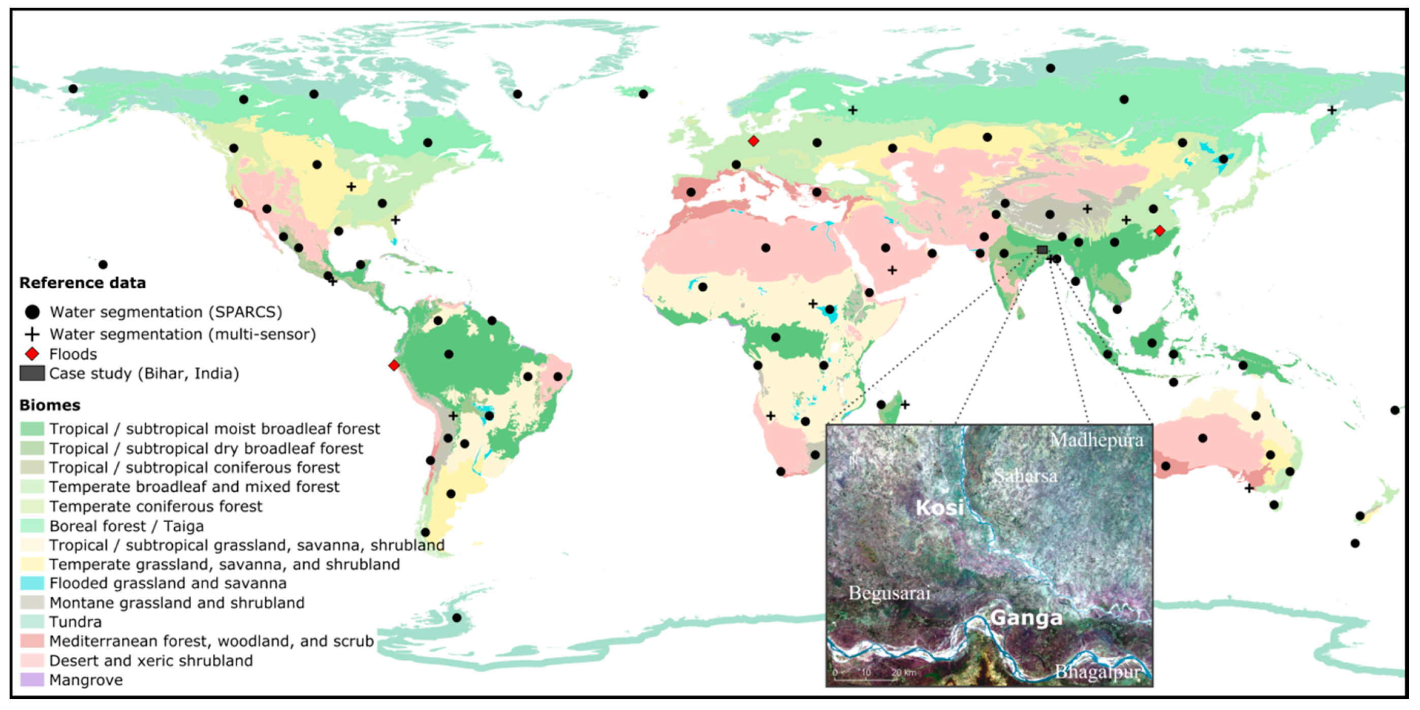
We compile a reference dataset based on globally distributed Landsat TM, ETM+, OLI and Sentinel-2 images to train, test and validate the water segmentation method (details about data ingestion and supported sensors are provided in Section 3.1.). For the dataset to be representative for a large variety of climatic, atmospheric, and land-cover conditions, we apply a stratified random sampling on the basis of a global biomes map [38] with a minimum distance constraint of 370 km (this equals twice the swath width of a Landsat scene) and pick 14 sample locations, for which we acquire respective imagery from each sensor (Figure 1). Acquisition times cover different seasons, subsets always cover water bodies amongst other land-cover classes and the minimum cloud-cover percentage for image acquisitions is set to 5 % to guarantee a minimum degree of cloud-cover per sample. We resample all imagery to 30 m spatial resolution, create a 1024 × 1024 pixels subset from each scene, stack the image bands together and convert Digital Numbers (DN) to Top of Atmosphere (TOA) reflectance (details about data preparation are provided in Section 3.2.). Thematic masks are manually delineated into classes “water”, “snow/ice”, “land”, “shadow”, and “cloud” based on image interpretation by an experienced operator. We further add the freely available Spatial Procedures for Automated Removal of Cloud and Shadow (SPARCS) dataset [39]. Similar to our multi-sensor dataset, it is globally sampled and consists of Landsat OLI images with corresponding manually delineated thematic masks.
We split all images and masks into non-overlapping tiles with 256 × 256 pixels size. The tiles are shuffled and divided into training (60 %), validation (20 %) and testing (20 %) datasets. The training dataset is further augmented with random contrast, brightness, gamma and rotation. Factors are randomly applied within predefined ranges to contrast [−0.4, 0.4], brightness [−0.2, 0.2] and gamma [0.5, 1.5]. Rotation is performed in steps of 90 degrees zero or more times. All augmentations are applied with equal probability. The final dataset covers 94 locations, 136 images from four sensors, and is split into 1075 tiles for training (5375 tiles with augmentations) and 358 tiles for validation and testing respectively.
To specifically test the flood mapping module, we select three flood disasters, for which very high-resolution optical data and imagery of one of the satellite sensors that we consider in this study are available (Figure 1). High and very high resolution optical data are used as independent reference, from which we manually delineate flood extent masks by means of a standard rapid mapping workflow. Reference and input images are not acquired more than two days apart from each other and visual checks are performed to assure that water extents are comparable. Cloud and cloud shadow pixels are masked in both reference and predicted masks and excluded from accuracy assessments. We analyse the following flood disasters:
- Germany, June 2013: As a result of a combination of wetness caused by a precipitation anomaly in May 2013 and strong event precipitation, large parts of Southern and Eastern Germany were hit by flooding [40]. In response to this, the International Charter “Space and Major Disasters” has been activated on June 2 [41] and emergency mapping has been conducted jointly by DLR’s Centre for Satellite-based Crisis Information (ZKI) and the Copernicus Emergency Management Service of the European Commission [42]. We use a Pléiades image (0.5 m) acquired on 08.06.2013 as basis to delineate the reference flood mask and a Landsat OLI image (30 m) from 07.06.2013 as input for the prediction. A pre-disaster Landsat OLI image from 20.04.2013 is used to generate the reference water mask.
- China, June 2016: Abnormally heavy monsoon rainfall intensified by a long and strong El Niño event caused flooding in the Yangtze River basin, which severely impacted the region’s economy and population [43]. In response to this, the International Charter “Space and Major Disasters” has been activated on 21.06.2016 [44]. We use a RapidEye image (5 m) acquired on 23.06.2016 as basis to delineate the reference flood mask and a Landsat OLI image (30 m) from the same date as input for the prediction. One Landsat OLI image for each of the 12 months before the disaster is used as input to generate the respective reference water mask.
- Peru, March 2017: A strong local El Niño weather pattern off the coast of Peru triggered heavy torrential rainfall that caused floods and mudslides with devastating impacts throughout the country [45]. In response to this, the International Charter “Space and Major Disasters” has been activated on 31.03.2017 [46]. We use a RapidEye image (5 m) acquired on 01.04.2017 as basis to delineate the reference flood mask and a Sentinel-2 image (10 m) from 31.03.2017 as input for the prediction. One Sentinel-2 image for each of the 12 months before the disaster is used as input to generate the respective reference water mask.
Furthermore, we define a case study for systematic flood monitoring in Bihar, India (Section 5). For the year 2018 all available Landsat OLI (19 images) and Sentinel-2 data (61 images) are acquired, processed and analysed with the proposed flood processing chain (Section 3). One Sentinel-2 image for each month of the previous year is used to generate the respective reference water mask. Moreover, for every month of the monitoring period one water segmentation mask per sensor is randomly selected for accuracy assessment. The 24 predicted masks are compared against reference point samples that are manually labelled by an experienced operator based on visual interpretation of the respective input images. A stratified random sample with minimum distance constraint of 250 m is used to identify the reference point locations for each predicted mask.
3. Method
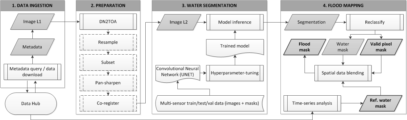
Figure 2 shows a schematic overview of the processing chain and its modules. Metadata and images are harvested from various sources and ingested into the processing chain for preparation and analysis (Section 3.1). The raw image bands are stacked and converted from DN to TOA reflectance values. Further preparation steps are added depending on the particular task and study area at hand (Section 3.2). The pre-processed image is fed into a trained CNN for water segmentation that produces a sematic segmentation of the image into five classes (Section 3.3). By reclassification of the segmentation result, we derive binary masks for water and valid pixels. A binary reference water mask is derived from time-series analysis of archive imagery and used to further distinguish reference water bodies from flood water (Section 3.5). Hence, the final outputs of the processing chain are binary flood, valid pixel, and reference water masks.
3.1. Data Ingestion
Table 1 provides an overview of the sensors currently supported by the processing chain. Landsat images are ingested at processing level L1TP from the USGS EarthExplorer data hub, which are radiometrically calibrated and orthorectified using ground control points and digital elevation model data to correct for relief displacement. Sentinel-2 images are ingested from the ESA Copernicus Open Access Hub at comparable processing level L1C, which are radiometrically calibrated, orthorectified and delivered in tiles of 100 × 100 km. Due to inconsistent availability and long processing times (resulting in longer lag times between satellite image acquisition and distribution), we decided against using imagery at higher processing levels, which are atmospherically corrected and delivered as surface reflectance products (e.g., Sentinel-2 at L2A).
Access protocols and metadata models that are being used for archiving products differ between data providers. An overview of available satellite data providers, their access protocols and metadata models can be found in Chen, Zhou and Chen (2015) [47]. In this work, we query and ingest data into the processing chain via a custom Application Programming Interface (API) that is connected to a set of Python scripts, which interface with the different sources, adjust metadata requests, harmonize responses and perform the actual data access through the source specific protocols. Along with each dataset, we store a harmonized metadata file in JSON-format, which contains all tags that are needed for rapid local data searches, documentation of processing history, and parameters for sensor specific transformations.
3.2. Preparation
Image preparation is done in succeeding steps. The combination and order of steps may vary depending on desired area of interest, geometric accuracy, spatial resolution, and sensor. Since all image data are delivered in single band raster files with varying grid size, we first resample them to the same grid size. Optionally, pan-sharpening is applied for sensors that provide a higher resolution panchromatic band. We use cubic convolution interpolation during resampling and a weighted Brovey transform for pan-sharpening [48]. All spectral bands are stacked together into a single dataset along the z-axis and optionally subset to a geographical area of interest along x- and y-axis. In this work, we only use spectral bands that are available across different satellite sensors to ensure a high degree of transferability of the trained water segmentation model (Section 3.3). Specifically, we use bands Red, Green, Blue, Near-Infrared (NIR) and two Shortwave-Infrared bands (SWIR1 and SWIR2). We transform DN to TOA reflectance using sensor specific methods. Image co-registration is performed using an algorithm based on Fast Fourier Transform (FFT) for translation, rotation and scale-invariant image registration [49]. For the study areas that are considered in the following, we found that all relevant images were already well registered to each other and an additional co-registration step was not necessary. The need for co-registration should, however, be evaluated on a case by case basis. An in-depth evaluation of inter- and intra-sensor image co-registration and a discussion about its necessity for Landsat and Sentinel-2 images are beyond the scope of this study but can be found in Stumpf, Michea and Malet (2018) [50].
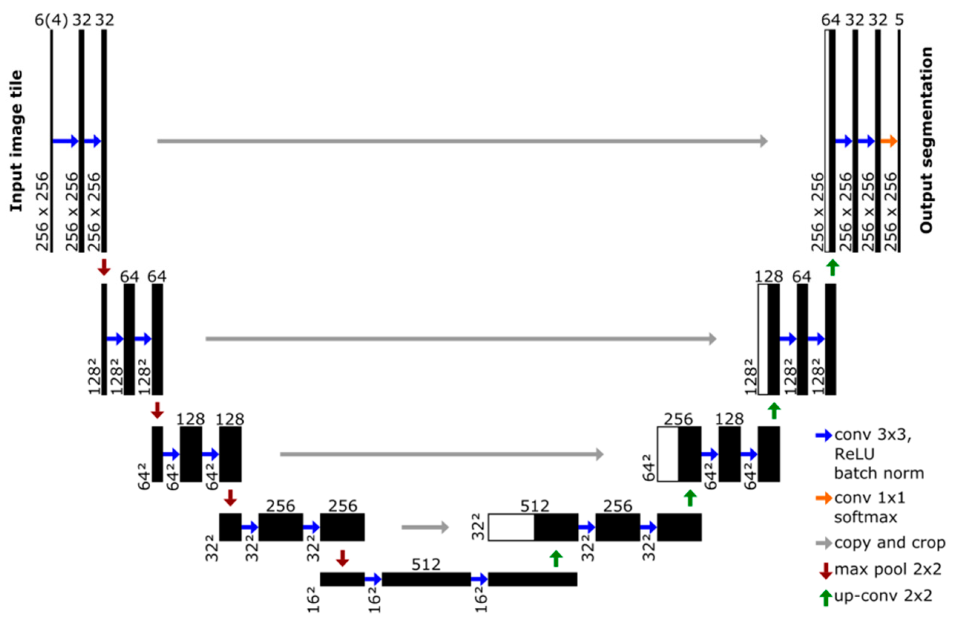
3.3. Water Segmentation with a Convolutional Neural Network
For semantic segmentation of water bodies we use a CNN based on the U-Net architecture [51] (Figure 3). The network achieved good accuracies for cloud and cloud shadow segmentation in previous work of the authors [12]. In this study, we retrain it on a multi-sensor dataset and optimize training towards improving the performance of the water segmentation. The network consists of encoder and decoder parts, where the encoder takes an input image and generates a high-dimensional feature vector with aggregate features at multiple scales. In five convolutional blocks we apply two 3 × 3 convolutions with Rectified Linear Unit (ReLU) activation function, followed by batch normalization and a 2 × 2 max pooling operation with stride 1 for down-sampling. In each block the number of feature channels is doubled starting from 32. In the decoder part, the feature map is up-sampled by a 2 × 2 transpose convolution followed by a concatenation with the correspondingly cropped feature map from the decoder and two 3 × 3 convolutions with ReLU activation and batch normalization. At the final layer a 1 × 1 convolution with softmax activation function is used to map each feature vector to the desired number of classes.
Compared to our previous study on cloud and cloud shadow segmentation, for which we trained a U-Net on the Landsat OLI SPARCS dataset [39], we train the water segmentation network on a larger multi-sensor dataset and apply more extended augmentation (Section 2). Image augmentation helps the network to learn invariance to changes in the augmented domains [52]. This is particularly relevant for remote sensing images, which are affected by a combination of a large variety of highly dynamic external (e.g., atmospheric conditions, seasonality) and internal (e.g., sensor characteristics) parameters.
To account for class imbalance, we use a weighted categorical cross-entropy loss function as defined in Equation (1) with being the weight, the true probability and the predicted probability for class i.
The weight vector is defined over the range of class labels and is computed on the training dataset for each class as the ratio of the median class frequency and the class frequency (Equation (2)).
The loss function assigns a higher cost to misclassification of smaller classes (e.g., “water”) and therefore reduces bias of the model by classes with relatively higher occurrence in the training dataset (e.g., “land”). The input image feature space is standardized to zero mean and unit variance with mean and standard deviation being computed on the training dataset and applied to the validation and testing datasets. The training set is shuffled once between every training epoch. We optimize the weights during training using the adaptive moment estimation (Adam) algorithm [53] with default hyper-parameters , and an initial learning rate α = 10−4. Additionally, we step-wise reduce the learning rate by a factor of 0.5 if no improvement is seen for five epochs. For model evaluation we track weighted categorical cross-entropy loss and Dice coefficient (Figure 4). In order to account for the fact that our focus is on applications in the emergency response sector, where computation time is a critical performance criterion, we also report inference times (measured in seconds/megapixel). We use Keras with Tensorflow backend [54] as deep learning framework and train the network in batches of 20 until convergence. Training the multi-sensor dataset described in Section 2 takes approximately five hours on a NVIDIA M4000 GPU running on a standard desktop PC with Intel Xeon CPU E5-1630 v4 @ 3.7 GHz, four cores and 20 GB RAM.
U-Net makes predictions on small local windows, which may result in higher prediction errors towards the image borders. Therefore, during inference we expand the input image with mirror-padding, split it into overlapping tiles, run the predictions over batches of tiles, blend the prediction tiles to reconstruct the expanded input image’s x-y-shape and un-pad the resulting prediction image. We use a tapered cosine window function (Equation (3)) to weight pixels when blending overlapping prediction tiles together, where N is the number of pixels in the output window and α is a shape parameter that represents the fraction of the window inside the cosine tapered region.
The final categorical output y is computed by maximizing the corresponding predicted probability vector p(x) (Equations (4) and (5)) with being the probability of x to belong to class i.
GPU inference speed computed over 358 test image tiles is 0.41 s/megapixel. This means that a Sentinel-2 image tile at 10 m spatial resolution with a typical size of 10,980 × 10,980 pixels can be analysed in approximately 50 s. Given the available hardware, this increases to roughly 40 min when inference is run on CPU.
3.4. Benchmark Water Segmentation
As benchmark for the proposed water segmentation method, we also train a traditional Random Forest classifier on the same standardized training dataset. Random Forest is widely used for water segmentation in multi-spectral satellite images [21,55]. We use the Scikit-learn [56] implementation of the classifier, which fits a number of optimized C4.5 decision tree classifiers [57] on sub-samples of the training data and uses averaging to control over-fitting. We tune hyper-parameters (in particular the number of trees in the forest and the number of features used at each node) according to a ten-fold cross-validation and grid-search method during the training phase of the classifier. Training the multi-sensor dataset takes approximately 5 min on CPU (the implementation used in this study does not support GPU computation). CPU inference speed computed over 358 test image tiles is 2.15 s/megapixel. This means that a typical Sentinel-2 image tile can be analysed in roughly 4 min when inference is run on CPU with four cores.
Additionally, we also compare the outcomes of our U-Net model against a simple NDWI thresholding method. For the water index z we iteratively change the threshold v over the whole range of index values (Equation (6)) and compare the predicted binary water masks with the true masks.
Since this method can only predict binary water/no water masks, we reclassify the categorical outputs of U-Net and Random Forest methods to match these binary masks before comparing them. For further comparison, we apply a widely used empirical threshold of v = 0.0 to produce binary water masks. This method is rule-based and does not need any training. CPU inference speed over 358 test images is 0.003 s/megapixel when setting a static threshold. This means that a Sentinel-2 image tile can be analysed in less than one second.
3.5. Flood Mapping
Multi-spectral satellite images are affected by clouds and shadows which may obstruct objects or areas of interest. It is therefore crucial for unbiased down-stream analysis to separate invalid from valid pixels. Accordingly, we reclassify the categorical output y produced by the water segmentation method (Equation (5)) to generate a binary valid pixel mask where “shadow”, “cloud” and “snow/ice” classes refer to “invalid” pixels, and “water” and “land” classes to “valid” pixels. Dilating the inverse of this mask with a 4 × 4 square-shaped structuring element k effectively buffers invalid pixels while taking its inverse provides us with the final valid pixel mask (Equation (7)).
To generate a binary water mask we reclassify the categorical output y (Equation (5)) such that “shadow”, “cloud”, “snow/ice” and “land” classes refer to “no water”, while the “water” class remains untouched. Intersecting this mask with the buffered valid pixel mask provides the final water mask (Equation (8)).
We further derive a reference water mask that aims at approximating the normal water extent and is used to separate temporarily flooded areas from permanent water bodies. To avoid bias by the choice of a single pre-flood image, we use a time-series of pre-flood images. Within a pre-defined time range (e.g., one year) before the acquisition date of the flood image, we derive binary water and valid pixel masks for all available imagery. Additional constraints may be set to identify relevant images, such as minimum cloud coverage or temporal granularity (e.g., use only one image per month). The relative water frequency f, with which water is present throughout the time-series is computed as defined in Equation (9), with being the binary water mask and the valid pixel mask at time step .
A permanent water pixel would be classified as belonging to class “water” in all valid observations throughout the time range, which would result in a relative water frequency f = 1.0. We relax the threshold for permanent water pixels and set it to f ≥ 0.9 according to the U-Net model performance for class “water” on the test dataset (Table 2) to account for uncertainties in the single water segmentations. This means that a pixel is identified as being permanent water if it belongs to class “water” in 90 % or more of the valid observations during a given time range. Finally, the set difference of the water mask derived from the flood image and the reference water mask r produces the final flood mask (Equation (10)).
It should be noted that the parameter values, which define the reference water mask (time range, temporal granularity, minimum cloud coverage, and relative water frequency threshold) depend on several rather subjective decisions and may be answered differently according to the specific application focus (e.g., disaster response, re-insurance, preparedness, etc.,) and the climatic and hydrologic conditions of the study area. A sensitivity analysis of these parameters is beyond the scope of this study but will be tackled in future work along with an in-depth evaluation of end-user’s needs and comparison of different reference water masking approaches.
4. Results
Figure 5 and Table 2 show summaries of the results for the proposed U-Net model and a Random Forest classifier. It can be seen that the U-Net model outperforms the Random Forest classifier with respect to all evaluation metrics across the globally distributed 358 test tiles. U-Net shows improvements of Overall Accuracy (OA) by 0.07, Kappa by 0.13 and Dice coefficient by 0.04 compared to Random Forest. U-Net also consistently produces higher F1-scores for all classes. The least accurate class in both models is the “shadow” class, which is mainly affected by confusions with the “land” class. In case of Random Forest this effect is significantly higher and affected by confusion with the “water” class. Moreover, Random Forest seems to have problems to segment “cloud” from “land”. A qualitative comparison of the results for selected test tiles confirms these findings across all tested satellite sensors (Figure 6).
To compare U-Net and Random Forest models with the NDWI thresholding method, we reclassify the categorical outputs of U-Net and Random Forest methods to match the binary classification scheme produced by thresholding the NDWI. From the Receiver Operating Characteristic (ROC) curves for class “water” (Figure 7) it can be seen that over all thresholds NDWI performs well (area under the curve (AUC) = 0.947), despite lacking behind Random Forest (AUC = 0.974) and U-Net (AUC = 0.995) models. When we apply a single threshold to the NDWI (in this case we use v = 0.0, which has been empirically defined and is referenced in many studies) the performance difference to the other methods becomes more prominent (Table 3). With respect to the simple NDWI thresholding, the best performing U-Net model shows an improvement for OA of 0.06, Kappa of 0.29 and Dice coefficient of 0.26. A qualitative comparison of the results confirms these findings across all tested satellite sensors (Figure 6). Moreover, it can be seen that the NDWI thresholding falsely identifies “shadow” pixels as “water” and “cloud” pixels as “land”.
The multi-sensor reference dataset contains only a single water class that does not specifically cover flood water. To evaluate the results of the model on flood water and to exemplify the flood mapping method, we analyse three globally distributed flood disasters, for which we acquired reference data by manually delineating water masks on the basis of independent high and very high resolution optical imagery (Section 2). To account for the highly dynamic surface water environments of the China and Peru scenes, we derive reference water masks from 12 images (Landsat OLI for China and Sentinel-2 for Peru) that are acquired during the year previous to the respective flood disaster. We select one image per month where cloud-cover is lowest, derive a flood frequency map from the predicted water extents and threshold it with f ≥ 0.9 to create the actual reference water masks. We use only a single pre-event image (Landsat OLI) to define the reference water extent, because surface water dynamics in the Germany scene are known to be stable under normal meteorological conditions. Table 4 shows the results of the independent accuracy assessment. Figure 8 depicts the input images and predicted flood maps.
It can be seen that water bodies can be segmented with consistently high OA (≥ 0.92), Kappa (≥ 0.86) and Dice coefficient (≥ 0.90), despite varying sensors, atmospheric conditions, seasons, locations and land-use/land-cover situations. The water segmentation method performs well in areas of permanent water with high F1-scores (≥ 0.93) throughout all test scenes. In potentially flooded areas the water segmentation decreases in performance with F1-scores between 0.88 and 0.90.
The Landsat OLI scene of Germany covers an area of 550 km2 and depicts inundated areas of the Elbe River in and around the city of Magdeburg. It is located in a temperate broadleaf and mixed forest biome. We can observe highly diverse land-use/land-cover in this urban-rural setup, including different types of residential, industrial, agriculture, forest and bare soil classes. Water body types include rivers, ponds, lakes and flood water of varying depth. Particular for this scene is the presence of flood water in urban areas and large stretches of flooded vegetation. The predicted flood and permanent water bodies match well with the manually delineated mask and the model is able to produce high precision (≥0.83) and recall (≥0.96) for both classes, despite the difficulties introduced by mixed spectral responses at sub-pixel resolution in flooded urban and vegetated areas. It takes the processing chain approximately 1 min to produce the final flood product, considering data preparation, water segmentation and flood mapping (including the generation of a reference water mask from a single pre-event image).
The cloud-free Landsat OLI image of China covers an area of 630 km2 and shows a stretch of the Yangtze River around the city of Poyang. The scene is located in a temperate broadleaf and mixed forest biome and displays a large variety of land-use/land-cover types including urban residential, industrial, agriculture and bare soil. Water body types include rivers, ponds, natural and artificial lakes and waterways, aquaculture and large areas of shallow to deep flood water. The model segments flood and permanent water with high precision (≥ 0.79) and recall (≥ 0.99) values and allows to quickly gain a detailed overview of the flood situation in this highly complex scene. It takes the processing chain approximately 6 min to produce the final flood product, considering data preparation, water segmentation and flood mapping (including the generation of a reference water mask from 12 pre-event images).
The Sentinel-2 image of Peru covers an area of 630 km2 and depicts a coastal area with large patches of ocean, estuaries and temporary flooded lagoons. Except for a few small settlements along the coastline, with the biggest being the village of Parachique, the area covered by this scene appears to be largely uninhabited. Dominating land-use/land-cover classes of this xeric shrubland biome include bare soil, sand and sparse vegetation. Along the main estuary smaller patches of flooded aquaculture can be observed. The scene shows the most complex atmospheric conditions with partially thick cloud cover and a large variety of different cloud types and respective cloud shadows. Nevertheless, the model is able to segment these as invalid pixels and remove them from further analysis. Despite the variety of water types, all visible water bodies can be delineated with high precision (≥ 0.87) and recall (≥ 0.93) for both permanent and flood water. It takes the processing chain approximately 6 min to produce the final flood product, considering data preparation, water segmentation and flood mapping (including the generation of a reference water mask from 12 pre-event images).
5. Flood Monitoring Application
A subset (100 × 100 km) of the Indian state of Bihar (Figure 1) is identified as study area to test the capabilities of the processing chain to systematically monitor flood water extent over time. Bihar is seasonally affected by tropical monsoon rain and considered to be one of the most flood prone regions in India [37]. Its plains are drained by a number of rivers that have their catchments in the Himalayas. The largest rivers in the study area are Ganga and Kosi. Highest water levels are usually recorded between June and October, when more than 80% of annual rain falls. Dominating land-use/land-cover classes of this tropical and subtropical moist broadleaf forest biome include vast areas of small scale agricultural fields with a variety of crops and growing patterns, patches of forest, wetlands and settlements of largely rural character. Along the major rivers large areas of temporary flooded bare soil and sand are present. The scene is affected by highly varying atmospheric conditions with a large variety of different cloud types and cloud shadows. For the year 2018 a total of 80 images from Landsat OLI and Sentinel-2 are accessed, processed and analysed with the flood processing chain. Additionally, 12 Sentinel-2 images for the year 2017 (one per month) are processed to generate a reference water mask with a relative water frequency threshold of f ≥ 0.9. Figure 9 shows relative water frequencies for 2017 and 2018.
It can be seen that the study area is further characterised by highly dynamic surface water; even stretches of the major rivers change their path throughout the year and hence are not considered as being permanent water by the given setup. Moreover, the maximum water extent indicates extended annual flooding. The 2017 Bihar flood, which had severe impacts on population, economy and housing sector in the district [58], is well represented in the water frequency maps with larger flood water extent being detected particularly along the Kosi River compared to 2018.
Figure 10 shows the monthly mean ratio of flood to water pixels for 2018 along with examples of flood products at different seasons. The plot depicts well the annual water regime of the study area with highest water levels between July and October, and a dry period with low water levels between March and June.
To assess the accuracy of the flood mapping results over time, we randomly select one flood mapping product per month and sensor. Each of the 24 products is compared against randomly selected and manually labelled point samples. Table 5 shows the results of the flood product comparison against the test samples over all months and sensors. The assessment indicates very good performance with OA, Kappa and Dice coefficient values well above 0.9 and a good balance between precision and recall for all classes. Permanent water locations are segmented with marginally better F1-score than temporary flooded locations. Figure 11 shows performance metrics for predicted flood products over time grouped by sensor. Over the observed 12 months period the performance varies in the range of 0.2 Kappa for Landsat OLI and 0.13 Kappa for Sentinel-2 with higher values being achieved between April and August. Predictions on Landsat OLI and Sentinel-2 show comparable performance during the observation period with and for Landsat OLI and and for Sentinel-2 respectively.
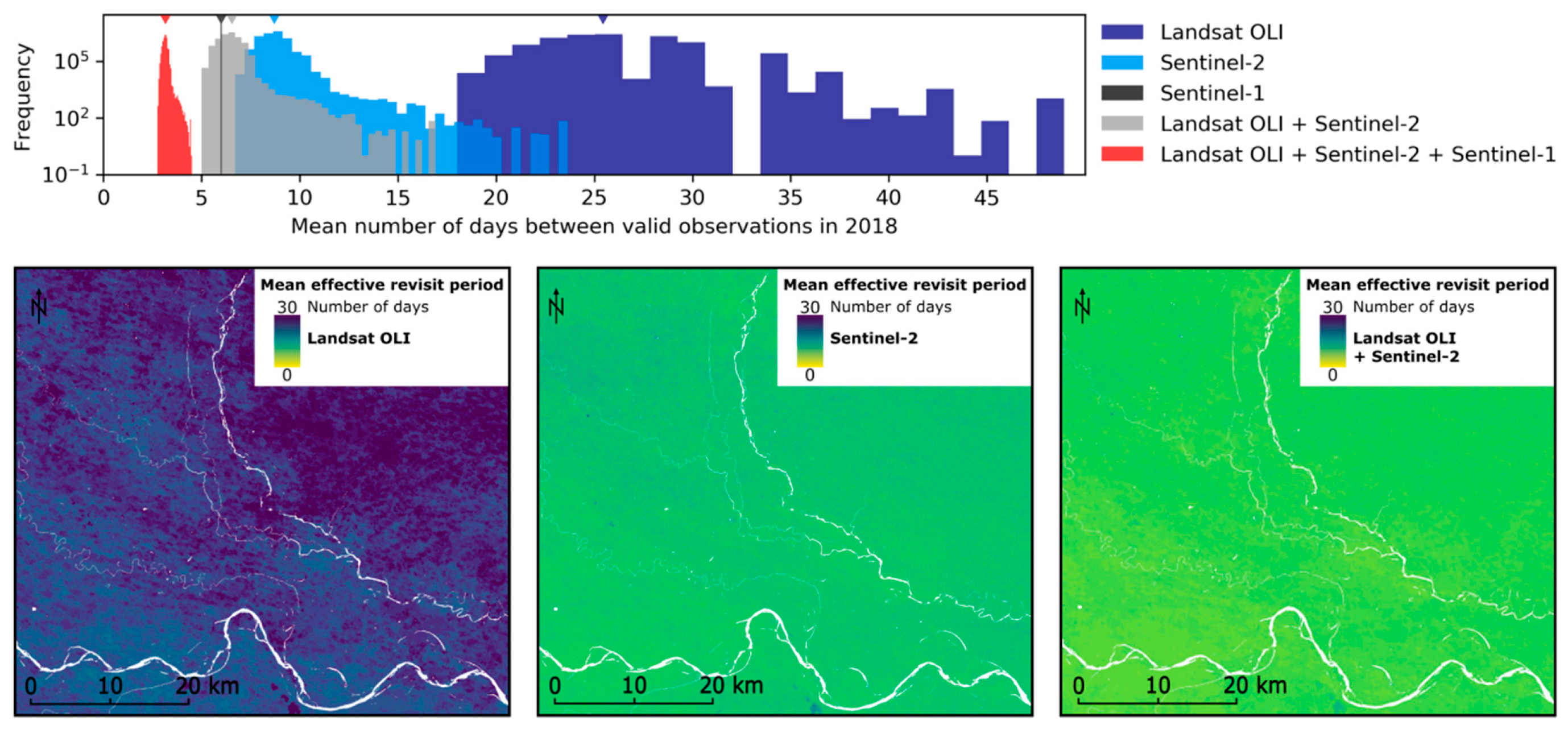
We further analyse the results with respect to the effective temporal revisit period that can be achieved with the given sensors under consideration of cloud coverage. For 2018 the spatial distribution and histograms of mean effective revisit periods (in number of days between valid observations) for different sensors and sensor combinations are provided in Figure 12. For each pixel in a stack of available images for a sensor combination and time range, we compute the time difference between succeeding acquisition dates for which the pixel is valid (e.g., not covered by cloud or cloud shadow). The maps visualize the mean over the time difference series, which is interpreted as the mean effective revisit period per pixel. The histograms depict the pixel value distribution over the study area with the respective median values being marked with triangles. This is summarized in Table 6, which compares the mean revisit periods with and without consideration of valid observations. Note that the satellite revisit period (considering all observations) has been computed specifically for the study area and may slightly differ from the revisit period provided by the satellite operators given in Table 1. For the multi-spectral sensors, the effective revisit period is consistently longer than the satellite revisit period due to cloud coverage. Since Sentinel-1 is a SAR sensor that penetrates through clouds, all pixels at all timestamps are considered to be valid. Consequently, the mean number of days between valid observations is the same for the whole study area and equals the mean satellite revisit period of six days. Combining Landsat OLI and Sentinel-2 can improve the effective revisit period by 2 days compared to using Sentinel-2 alone and by 19 days compared to Landsat OLI. Combining Sentinel-1 with the multi-spectral sensors can improve the effective revisit period to up to 3 days, which equals half the revisit period of Sentinel-1 over the study area.
The main aim of the water segmentation module is to train a model that generalizes well across different sensors, locations and atmospheric conditions. We proposed a CNN with U-Net architecture, which showed superior performance in terms of OA, Kappa and Dice coefficient compared to the benchmark methods (Random Forest and NDWI thresholding). We decided to use only spectral bands that are acquired by all tested sensors (Red, Green, Blue, NIR, SWIR1 and SWIR2 bands) to allow for a high degree of transferability across sensors. We specifically decided against using the Thermal Infrared (TIR) bands as these are not acquired by Sentinel-2. For sensor-specific applications, however, including TIR bands into the input feature space of the network may have a positive effect on the performance. The target domain is affected by atmospheric conditions, land-use/land-cover and other scene and image properties. Despite our aim to cover these natural and technical variations in the manually annotated reference dataset, we decided to apply image augmentation to artificially increase the training sample size and to cover a larger range of conditions that may occur during inference in real-world applications. The need for augmentation has been reinforced by experiments that were carried out in previous work of the authors [12]. We acquired a multi-sensor reference dataset that we used to train, validate and test the water segmentation. The reference dataset has been sampled globally under consideration of terrestrial biomes to account for a large variety of climatic, atmospheric and land-cover conditions. Samples are derived by manual interpretation and digitization of satellite image patches, which means that the results are to be regarded as relative to the performance of a human analyst and not to an absolute ground-truth. Especially clouds and cloud shadows lead to the problem of defining a hard class boundary on fuzzy borders. Their manual delineation is at least partially a matter of subjective interpretation and may introduce a bias in the reference dataset and hence into the performance results.
The Random Forest model shows problems to distinguish between “shadow” and “land” classes. Shadow prevents the spectral characteristics of the underlying surface from being fully represented, which may cause an overlap of the spectral signatures of shadow and land pixels. The U-Net model seems to largely overcome this by its non-linear function mapping capability and by the convolutional features that are being learned directly from the data under consideration of neighbourhood information at various scales. Considering only spectral characteristics of single pixels (like this is the case for the Random Forest model) seems to be insufficient. At least textural and/or spatial information would be needed to distinguish these classes. Computing additional hand-crafted features (e.g., based on Grey-Level Co-occurrence Matrix) over a sliding-window or as part of an object-based image analysis could improve the results for traditional machine learning models like Random Forest but would involve significantly longer computation time during inference. We also compared binary reclassifications of the CNN and Random Forest predictions against a widely used NDWI thresholding method. We could show that across all thresholds the NDWI method can produce good predictions but clearly lacks behind the machine learning methods. Particular problems include finding an optimal threshold that is globally applicable. Our experiments show, moreover, that even with an optimal threshold the NDWI feature space is not sufficient to distinguish water from certain other classes with similar spectral response characteristics like shadows. This means that under realistic conditions (images show divers cloud and shadow coverage) NDWI thresholding could only produce valid results, if a cloud and shadow mask is being applied beforehand. The other two methods deliver the respective segmentations directly.
Compared to other studies, our work presents an end-to-end solution that is targeted towards an operational usage. We focus specifically on multi-sensor generalization ability, simplicity and processing speed to produce timely, accurate and relevant information products for emergency responders in flood disaster situations. Isikdogan, Bovik and Passalacqua (2017) [26] use a Fully Convolutional Network to map surface water from Landsat ETM+. They train and test their model on independent subsets of the Global Land-cover Facility (GLCF) inland water dataset [19] but do not specifically target transferability between sensors. Similarly, to our study, their results show confusion between “cloud” and “land” as well as “water” and “shadow” classes. Despite using simpler network architecture and a smaller training dataset, our model is able to reduce these confusions. In a previous study, we have used the same network architecture for “cloud” and “cloud shadow” segmentation with “water” and other classes being byproducts [12]. In the present work, the training has been tuned towards refining the segmentation of water bodies. In particular, we have significantly increased the training dataset in terms of sensors, locations, and sample size. We apply more extended augmentation and use a weighted loss function to better account for underrepresented classes. These modifications could improve the performance of the U-Net model by 0.04 OA, 0.05 Kappa and 0.05 Dice coefficient. The “water” class shows an improvement in F1-score by 0.08 with an increase in precision of 0.18 at a decrease in recall of 0.03. In its current form the model considers cloud shadows but has not specifically been trained on other shadow types (e.g., terrain shadows). Despite the encouraging results achieved on the global test dataset, this may be a potential source of false-positives for water segmentation in mountainous areas with strong terrain shadow effects. Therefore, future work will focus on refining the training dataset and experimenting with different network architectures to further improve generalization ability and increase precision and recall. Further experiments are also planned to evaluate the effect of atmospheric correction on the performance. This becomes particularly relevant as the lag time between satellite image acquisition and distribution is expected to decrease for standardized atmospherically corrected data in coming years [59].
We present a pragmatic solution to derive a reference water mask for any given area and time of interest, which can be regarded as a step forward compared to the usually static approaches reported in literature. Despite the technical implementation that can be adapted to dynamic environments, it should be noted that its definition is not universal and may vary depending on the application, targeted end-users, geographical region and time period. An in-depth evaluation of use-cases and a more quantitative approach towards the definition of reference water and the respective decision about parameter settings is still pending. This is beyond the scope of this study and will be treated as a separate research in the future. However, for three flood disasters and a monitoring application we could show the potentials and flexibility of the proposed reference water mask and related flood product. In particular, we could show that flood and permanent water were segmented with high accuracies in all tested situations. A slight performance decrease for flood water could be observed, which is consistent with the effect that flood water commonly defines the maximum water extent and thus the land-water border. Particularly in flood situations this border can show highly complex patterns (e.g., submerged vegetation) that increase the complexity of the segmentation task compared to permanent water. Moreover, we could show that segmentation performance is comparable between sensors but varies over the observed 12 months period in the range of 0.2 Kappa for Landsat OLI and 0.13 Kappa for Sentinel-2. Marginally higher accuracies during monsoon months (April to August) may indicate a seasonal effect on the performance that may be triggered by increased cloud coverage. In order to confirm these findings, however, it would be needed to analyse a longer time-series and see if this effect persists.
We introduce the mean effective revisit period as a measure of how frequent a location on the ground is observed by a satellite during a given time range. Compared to the commonly referenced satellite revisit period, the effective revisit period specifically considers cloud and cloud shadow coverage. It is therefore a more meaningful measure to understand the applicability of a multi-spectral satellite sensor to provide valid observations during monitoring tasks. Naturally, the effective revisit period of optical sensors is longer than the satellite revisit period, because generally not all pixels in all acquisitions are cloud and cloud shadow free. It should be noted, however, that it is only valid for a given area and time range. Accordingly, results may vary for example if we set the time range around a specific season or if we change the study area. Nevertheless, we could show that the mean effective revisit period can significantly be improved by combining data from multiple sensors. For the study area in India the combination of systematically acquired multi-spectral and SAR data could reduce the mean effective revisit period to 3 days (compared to 6 days for Sentinel-1 only) in 2018. Therefore, the prototypical multi-spectral processing chain shows high potential to complement SAR-based flood services.
6. Conclusions
In this study, we introduced a modular processing chain for automated flood monitoring from multi-spectral satellite data. The presented prototype provides a complete solution to process raw image data into actionable information products that can provide rapid situational awareness in disaster situations. Performance evaluation showed that the implemented method produces highly accurate results and generalize well across different sensors, seasons, locations and disasters (0.93 OA, 0.87 Kappa, 0.90 Dice coefficient). Moreover, no atmospheric correction and ancillary datasets (e.g., digital elevation models) are required, which reduces complexity and allows for rapid processing. By successfully applying the processing chain to three exemplary flood disasters and to a flood monitoring application, we could highlight the usefulness of our work for emergency response in terms of inference speed (0.41 s/megapixel on a standard GPU), accuracy (≥ 0.92 OA, ≥ 0.86 Kappa, ≥ 0.90 Dice coefficient) and mean effective revisit period (6–7 days for multi-spectral only, 6 days for SAR only and 3 days for multi-spectral and SAR combined). We considered the most common systematically acquired high resolution multi-spectral satellite data, namely Landsat TM, ETM+, OLI and Sentinel-2. However, the modular structure of the processing chain allows for flexible extension to other sensors. Ongoing and future works focus on implementing support for additional high-resolution sensors (e.g., ALOS-AVNIR2, PlanetScope, etc.), and to train a water segmentation model for very high resolution satellite (e.g., Pléiades, Kompsat-3, etc.) and aerial imagery. Additional research is also needed regarding the definition of a reference water mask. In this context, it is intended to carry out an end-user knowledge elicitation to gain a better insight into their information needs and to define common use cases for the application of a reference water mask. More specifically, we should be able to setup a structured scheme that supports the choice of appropriate parameter settings (time range, granularity and additional constraints) in a less subjective manner and more targeted towards the needs of specific applications, locations and end-users’ needs. Furthermore, it is envisaged to elaborate upon the use of spatial uncertainty metrics that may be able to support decision making. Finally, the proposed processing chain will complement existing SAR-based flood monitoring services [5,6] to produce flood maps in an operational context with improved temporal revisit period.
Author Contributions
Conceptualization, M.W. and S.M.; methodology, M.W.; software, M.W.; validation, M.W.; formal analysis, M.W.; investigation, M.W.; data curation, M.W.; writing—original draft preparation, M.W.; writing—review and editing, M.W. and S.M.; visualization, M.W.; supervision, S.M.
Funding
This work was supported by the German Society for International Cooperation (GIZ) GmbH as part of the InsuResilience project (Grant No. 81220843) and the German Federal Ministry of Education and Research (BMBF) as part of the RIESGOS project (Grant No. 03G0876).
Acknowledgments
The authors would like to thank the editors and the anonymous reviewers for their constructive comments and suggestions that helped to improve this manuscript.
Conflicts of Interest
The authors declare no conflict of interest. The founding sponsors had no role in the design of the study; in the collection, analyses, or interpretation of data; in the writing of the manuscript, and in the decision to publish the results.
References
- Klemas, V. Remote sensing of floods and flood-prone areas: An overview. J. Coast. Res. 2015, 314, 1005–1013. [Google Scholar] [CrossRef]
- Voigt, S.; Giulio-Tonolo, F.; Lyons, J.; Kučera, J.; Jones, B.; Schneiderhan, T.; Platzeck, G.; Kaku, K.; Hazarika, M.K.; Czaran, L.; et al. Global trends in satellite-based emergency mapping. Science 2016, 353, 247–252. [Google Scholar] [CrossRef] [PubMed]
- Schumann, G.; Moller, D. Microwave remote sensing of flood inundation. Phys. Chem. Earth 2015, 83–84, 84–95. [Google Scholar] [CrossRef]
- Lin, L.; Di, L.; Yu, E.G.; Kang, L.; Shrestha, R.; Rahman, M.S.; Tang, J.; Deng, M.; Sun, Z.; Zhang, C.; et al. A review of remote sensing in flood assessment. In Proceedings of the 2016 Fifth International Conference on Agro-Geoinformatics (Agro-Geoinformatics), Tianjin, China, 8–20 July 2016; pp. 1–4. [Google Scholar]
- Martinis, S.; Kersten, J.; Twele, A. A fully automated TerraSAR-X based flood service. Isprs J. Photogramm. Remote Sens. 2015, 104, 203–212. [Google Scholar] [CrossRef]
- Twele, A.; Cao, W.; Plank, S.; Martinis, S. Sentinel-1-based flood mapping: A fully automated processing chain. Int. J. Remote Sens. 2016, 37, 2990–3004. [Google Scholar] [CrossRef]
- Hoersch, B.; Amans, V. Copernicus Space Component Data Access Portfolio: Data Warehouse 2014–2020; ESA: Frascati, Italy, 2014; p. 81. [Google Scholar]
- Main-Knorn, M.; Pflug, B.; Louis, J.; Debaecker, V.; Müller-Wilm, U.; Gascon, F. Sen2Cor for Sentinel-2. In Proceedings of the SPIE Image and Signal Processing for Remote Sensing XXIII, Warsaw, Poland, 11–13 September 2017; Bruzzone, L., Bovolo, F., Benediktsson, J.A., Eds.; Volume 10427, p. 3. [Google Scholar]
- Richter, R.; Schläpfer, D.; Müller, A. An automatic atmospheric correction algorithm for visible/NIR imagery. Int. J. Remote Sens. 2006, 27, 2077–2085. [Google Scholar] [CrossRef]
- Hagolle, O.; Huc, M.; Pascual, D.V.; Dedieu, G. A multi-temporal method for cloud detection, applied to FORMOSAT-2, VENµS, LANDSAT and SENTINEL-2 images. Remote Sens. Environ. 2010, 114, 1747–1755. [Google Scholar] [CrossRef]
- Zhu, Z.; Wang, S.; Woodcock, C.E. Improvement and expansion of the Fmask algorithm: Cloud, cloud shadow, and snow detection for Landsats 4–7, 8, and Sentinel 2 images. Remote Sens. Environ. 2015, 159, 269–277. [Google Scholar] [CrossRef]
- Wieland, M.; Li, Y.; Martinis, S. Multi-sensor cloud and cloud shadow segmentation with a convolutional neural network. Remote Sens. Environ. 2019, 230, 1–12. [Google Scholar] [CrossRef]
- Gao, B. NDWI—A normalized difference water index for remote sensing of vegetation liquid water from space. Remote Sens. Environ. 1996, 58, 257–266. [Google Scholar] [CrossRef]
- Xu, H. Modification of normalised difference water index (NDWI) to enhance open water features in remotely sensed imagery. Int. J. Remote Sens. 2006, 27, 3025–3033. [Google Scholar] [CrossRef]
- Wang, X.; Xie, S.; Zhang, X.; Chen, C.; Guo, H.; Du, J.; Duan, Z. A robust Multi-Band Water Index (MBWI) for automated extraction of surface water from Landsat 8 OLI imagery. Int. J. Appl. Earth Obs. Geoinf. 2018, 68, 73–91. [Google Scholar] [CrossRef]
- Feyisa, G.L.; Meilby, H.; Fensholt, R.; Proud, S.R. Automated Water Extraction Index: A new technique for surface water mapping using Landsat imagery. Remote Sens. Environ. 2014, 140, 23–35. [Google Scholar] [CrossRef]
- Zhou, Y.; Dong, J.; Xiao, X.; Xiao, T.; Yang, Z.; Zhao, G.; Zou, Z.; Qin, Y. Open Surface Water Mapping Algorithms: A Comparison of Water-Related Spectral Indices and Sensors. Water 2017, 9, 256. [Google Scholar] [CrossRef]
- Du, Y.; Zhang, Y.; Ling, F.; Wang, Q.; Li, W.; Li, X. Water Bodies’ Mapping from Sentinel-2 Imagery with Modified Normalized Difference Water Index at 10-m Spatial Resolution Produced by Sharpening the SWIR Band. Remote Sens. 2016, 8, 354. [Google Scholar] [CrossRef]
- Feng, M.; Sexton, J.O.; Channan, S.; Townshend, J.R. A global, high-resolution (30-m) inland water body dataset for 2000: First results of a topographic–spectral classification algorithm. Int. J. Digit. Earth 2016, 9, 113–133. [Google Scholar] [CrossRef]
- Pekel, J.-F.; Cottam, A.; Gorelick, N.; Belward, A.S. High-resolution mapping of global surface water and its long-term changes. Nature 2016, 540, 418–422. [Google Scholar] [CrossRef]
- Ko, B.; Kim, H.; Nam, J. Classification of Potential Water Bodies Using Landsat 8 OLI and a Combination of Two Boosted Random Forest Classifiers. Sensors 2015, 15, 13763–13777. [Google Scholar] [CrossRef] [Green Version]
- Mueller, N.; Lewis, A.; Roberts, D.; Ring, S.; Melrose, R.; Sixsmith, J.; Lymburner, L.; McIntyre, A.; Tan, P.; Curnow, S.; et al. Water observations from space: Mapping surface water from 25 years of Landsat imagery across Australia. Remote Sens. Environ. 2016, 174, 341–352. [Google Scholar] [CrossRef]
- Hughes, M.; Hayes, D. Automated Detection of Cloud and Cloud Shadow in Single-Date Landsat Imagery Using Neural Networks and Spatial Post-Processing. Remote Sens. 2014, 6, 4907–4926. [Google Scholar] [CrossRef] [Green Version]
- Hollstein, A.; Segl, K.; Guanter, L.; Brell, M.; Enesco, M. Ready-to-Use Methods for the Detection of Clouds, Cirrus, Snow, Shadow, Water and Clear Sky Pixels in Sentinel-2 MSI Images. Remote Sens. 2016, 8, 666. [Google Scholar] [CrossRef]
- Yu, L.; Wang, Z.; Tian, S.; Ye, F.; Ding, J.; Kong, J. Convolutional Neural Networks for Water Body Extraction from Landsat Imagery. Int. J. Comput. Intell. Appl. 2017, 16, 1750001. [Google Scholar] [CrossRef]
- Isikdogan, F.; Bovik, A.C.; Passalacqua, P. Surface Water Mapping by Deep Learning. Ieee J. Sel. Top. Appl. Earth Obs. Remote Sens. 2017, 10, 4909–4918. [Google Scholar] [CrossRef]
- Gutman, G.; Byrnes, R.; Masek, J.; Covington, S. Towards Monitoring Changes at a Global The Global Land Su. Photogramm. Eng. 2008, 6. [Google Scholar]
- Chen, Y.; Fan, R.; Yang, X.; Wang, J.; Latif, A. Extraction of Urban Water Bodies from High-Resolution Remote-Sensing Imagery Using Deep Learning. Water 2018, 10, 585. [Google Scholar] [CrossRef]
- Nogueira, K.; Fadel, S.G.; Dourado, I.C.; Werneck, R.; Munoz, J.A.V.; Penatti, O.A.B.; Calumby, R.T.; Li, L.T.; dos Santos, J.A.; Torres, R.d.S.; et al. Exploiting ConvNet Diversity for Flooding Identification. Ieee Geosci. Remote Sens. Lett. 2018, 15, 1446–1450. [Google Scholar] [CrossRef]
- Byun, Y.; Han, Y.; Chae, T. Image Fusion-Based Change Detection for Flood Extent Extraction Using Bi-Temporal Very High-Resolution Satellite Images. Remote Sens. 2015, 7, 10347–10363. [Google Scholar] [CrossRef] [Green Version]
- Franci, F.; Mandanici, E.; Bitelli, G. Remote sensing analysis for flood risk management in urban sprawl contexts. Geomat. Nat. Hazards Risk 2015, 6, 583–599. [Google Scholar] [CrossRef]
- Rahman, Md.R.; Thakur, P.K. Detecting, mapping and analysing of flood water propagation using synthetic aperture radar (SAR) satellite data and GIS: A case study from the Kendrapara District of Orissa State of India. Egypt. J. Remote Sens. Space Sci. 2018, 21, S37–S41. [Google Scholar] [CrossRef]
- Van Leeuwen, B.; Tobak, Z.; Kovács, F.; Sipos, G. Towards a continuous inland excess water flood monitoring system based on remote sensing data. J. Environ. Geogr. 2017, 10, 9–15. [Google Scholar] [CrossRef] [Green Version]
- CORINE Land Cover. Available online: https://land.copernicus.eu/pan-european/corine-land-cover (accessed on 10 October 2018).
- NASA Shuttle Radar Topography Mission Water Body Data. Available online: https://lpdaac.usgs.gov/products/srtmswbdv003/ (accessed on 5 April 2018).
- Tulbure, M.G.; Broich, M.; Stehman, S.V.; Kommareddy, A. Surface water extent dynamics from three decades of seasonally continuous Landsat time series at subcontinental scale in a semi-arid region. Remote Sens. Environ. 2016, 178, 142–157. [Google Scholar] [CrossRef]
- Amarnath, G.; Matheswaran, K.; Pandey, P.; Alahacoon, N.; Yoshimoto, S. Flood Mapping Tools for Disaster Preparedness and Emergency Response Using Satellite Data and Hydrodynamic Models: A Case Study of Bagmathi Basin, India. Proc. Natl. Acad. Sci. India Sect. A Phys. Sci. 2017, 87, 941–950. [Google Scholar] [CrossRef]
- Olson, D.M.; Dinerstein, E.; Wikramanayake, E.D.; Burgess, N.D.; Powell, G.V.N.; Underwood, E.C.; D’amico, J.A.; Itoua, I.; Strand, H.E.; Morrison, J.C.; et al. Terrestrial Ecoregions of the World: A New Map of Life on Earth. BioScience 2001, 51, 933. [Google Scholar] [CrossRef]
- USGS L8 SPARCS Cloud Validation Masks. Available online: https://landsat.usgs.gov/sparcs (accessed on 4 July 2018).
- Schröter, K.; Kunz, M.; Elmer, F.; Mühr, B.; Merz, B. What made the June 2013 flood in Germany an exceptional event? A hydro-meteorological evaluation. Hydrol. Earth Syst. Sci. 2015, 19, 309–327. [Google Scholar] [CrossRef] [Green Version]
- The International Charter Space and Major Disasters - Flood Germany 2013. Available online: https://disasterscharter.org/web/guest/activations/-/article/floods-in-germany (accessed on 4 October 2018).
- Copernicus Emergency Mapping Service - EMSR044. Available online: https://emergency.copernicus.eu/mapping/list-of-components/EMSR044 (accessed on 4 October 2018).
- Yuan, Y.; Gao, H.; Li, W.; Liu, Y.; Chen, L.; Zhou, B.; Ding, Y. The 2016 summer floods in China and associated physical mechanisms: A comparison with 1998. J. Meteorol. Res. 2017, 31, 261–277. [Google Scholar] [CrossRef]
- The International Charter Space and Major Disasters - Flood China 2016. Available online: https://disasterscharter.org/web/guest/activations/-/article/flood-in-chi-6 (accessed on 4 October 2018).
- Ramírez, I.J.; Briones, F. Understanding the El Niño Costero of 2017: The Definition Problem and Challenges of Climate Forecasting and Disaster Responses. Int. J. Disaster Risk Sci. 2017, 8, 489–492. [Google Scholar] [CrossRef]
- The International Charter Space and Major Disasters - Flood Peru 2017. Available online: https://disasterscharter.org/web/guest/activations/-/article/flood-in-peru-call-602- (accessed on 4 October 2018).
- Chen, N.; Zhou, L.; Chen, Z. A Sharable and Efficient Metadata Model for Heterogeneous Earth Observation Data Retrieval in Multi-Scale Flood Mapping. Remote Sens. 2015, 7, 9610–9631. [Google Scholar] [CrossRef] [Green Version]
- Pohl, C.; Van Genderen, J.L. Multisensor image fusion in remote sensing: Concepts, methods and applications. Int. J. Remote Sens. 1998, 19, 823–854. [Google Scholar] [CrossRef]
- Reddy, B.S.; Chatterji, B.N. An FFT-based technique for translation, rotation, and scale-invariant image registration. Ieee Trans. Image Process. 1996, 5, 1266–1271. [Google Scholar] [CrossRef]
- Stumpf, A.; Michéa, D.; Malet, J.-P. Improved Co-Registration of Sentinel-2 and Landsat-8 Imagery for Earth Surface Motion Measurements. Remote Sens. 2018, 10, 160. [Google Scholar] [CrossRef]
- Ronneberger, O.; Fischer, P.; Brox, T. U-Net: Convolutional Networks for Biomedical Image Segmentation. In Medical Image Computing and Computer-Assisted Intervention—MICCAI 2015; Navab, N., Hornegger, J., Wells, W.M., Frangi, A.F., Eds.; Springer International Publishing: Cham, Switzerland, 2015; Volume 9351, pp. 234–241. ISBN 978-3-319-24573-7. [Google Scholar]
- Dosovitskiy, A.; Springenberg, J.T.; Brox, T. Unsupervised feature learning by augmenting single images. arXiv 2014, arXiv:1312.5242. [Google Scholar]
- Kingma, D.P.; Lei, J. Adam: A Method for Stochastic Optimization. arXiv 2015, arXiv:1412.6980v9. [Google Scholar]
- Keras. Available online: https://keras.io (accessed on 14 June 2018).
- Acharya, T.; Lee, D.; Yang, I.; Lee, J. Identification of Water Bodies in a Landsat 8 OLI Image Using a J48 Decision Tree. Sensors 2016, 16, 1075. [Google Scholar] [CrossRef] [PubMed]
- Scikit-learn. Available online: http://scikit-learn.org (accessed on 8 May 2018).
- Breiman, L. Random Forests. Mach. Learn. 2001, 45, 5–32. [Google Scholar] [CrossRef] [Green Version]
- Floodlist—Flood Bihar 2017. Available online: http://floodlist.com/asia/india-floods-bihar-august-2017 (accessed on 4 October 2018).
- Claverie, M.; Ju, J.; Masek, J.G.; Dungan, J.L.; Vermote, E.F.; Roger, J.-C.; Skakun, S.V.; Justice, C. The Harmonized Landsat and Sentinel-2 surface reflectance data set. Remote Sens. Environ. 2018, 219, 145–161. [Google Scholar] [CrossRef]
Figure 1.
Sample locations of the reference dataset used for training, testing and validation of the water segmentation method; biome map used as strata for sampling; spatial distribution of the flood disasters used for independent testing; and overview of the case study area for systematic flood monitoring.

Figure 2.
Overview of the processing chain for automated flood monitoring from multi-spectral satellite data.
Figure 2.
Overview of the processing chain for automated flood monitoring from multi-spectral satellite data.

Figure 3.
Architecture of the U-Net used in this study.

Figure 4.
Visualization of the U-Net training history with training and validation loss and dice coefficient.
Figure 4.
Visualization of the U-Net training history with training and validation loss and dice coefficient.

Figure 5.
Error matrices for U-Net and Random Forest multi-class segmentation over the 358 test tiles for Landsat TM, ETM+, OLI and Sentinel-2.
Figure 5.
Error matrices for U-Net and Random Forest multi-class segmentation over the 358 test tiles for Landsat TM, ETM+, OLI and Sentinel-2.

Figure 6.
Examples of Landsat TM, ETM+, OLI and Sentinel-2 test image tiles with respective multi-class reference mask, U-Net and Random Forest segmentations and Normalized Difference Water Index (NDWI) thresholding water mask.
Figure 6.
Examples of Landsat TM, ETM+, OLI and Sentinel-2 test image tiles with respective multi-class reference mask, U-Net and Random Forest segmentations and Normalized Difference Water Index (NDWI) thresholding water mask.

Figure 7.
Receiver Operating Characteristic (ROC) curves for the water class comparing U-Net, Random Forest and NDWI thresholding over the 358 test tiles for Landsat TM, ETM+, OLI and Sentinel-2.
Figure 7.
Receiver Operating Characteristic (ROC) curves for the water class comparing U-Net, Random Forest and NDWI thresholding over the 358 test tiles for Landsat TM, ETM+, OLI and Sentinel-2.

Figure 8.
Satellite images of flood disasters with respective results of the flood mapping method.

Figure 9.
Relative water frequency over the study area Bihar derived from 12 monthly Sentinel-2 images for the reference year 2017 (left) and from 80 Landsat OLI and Sentinel-2 images for 2018 (right).
Figure 9.
Relative water frequency over the study area Bihar derived from 12 monthly Sentinel-2 images for the reference year 2017 (left) and from 80 Landsat OLI and Sentinel-2 images for 2018 (right).

Figure 10.
Monthly mean ratio of flood to water pixels for 2018 with flood processing results for selected timestamps.
Figure 10.
Monthly mean ratio of flood to water pixels for 2018 with flood processing results for selected timestamps.

Figure 11.
Overall accuracy, Kappa and Dice coefficient of 24 randomly selected flood mapping products over time grouped by sensor.
Figure 11.
Overall accuracy, Kappa and Dice coefficient of 24 randomly selected flood mapping products over time grouped by sensor.

Figure 12.
Spatial distribution of mean effective revisit periods with histograms (in number of days between valid observations) in 2018 for Landsat OLI, Sentinel-2, Sentinel-1, Landsat OLI + Sentinel-2 combined and Landsat OLI + Sentinel-2 + Sentinel-1 combined. The reference water mask is superimposed in white as orientation guide.6. Discussion.


Table 1.
Image characteristics of the sensors that are supported by the processing chain.
| Sensor | Spatial Res. (Swath) | Spectral Res. (Wavelength) | Revisit Period | Availability | Format | Source |
|---|---|---|---|---|---|---|
| Landsat TM | 30, 120 m (185 km) | Blue, Green, Red, NIR, SWIR1, SWIR2, TIR (0.45–12.50 µm) | 16 days | 1984–2013 | GeoTIFF (8 bit) | USGS |
| Landsat ETM+ | 15, 30, 60 m (185 km) | Blue, Green, Red, NIR, SWIR1, SWIR2, TIR, PAN (0.45–12.50 µm) | 16 days | 1999–now | GeoTIFF (8 bit) | USGS |
| Landsat OLI/TIR | 15, 30, 100 m(185 km) | AEROSOL, Blue, Green, Red, NIR, SWIR1, SWIR2, TIR1, TIR2, PAN, CIRRUS (0.43–12.51 µm) | 16 days | 2013–now | GeoTIFF (12 bit) | USGS |
| Sentinel-2 MSI | 10, 20, 60 m (290 km) | AEROSOL, Blue, Green, Red, RedEdge1, RedEdge2, RedEdge3, NIR, RedEdge4, VAPOUR, CIRRUS, SWIR1, SWIR2 (0.44–2.19 µm) | 5 days | 2015–now | JPEG2000 (12 bit) | ESA |
Table 2.
Per-class comparison between U-Net and Random Forest models over the 358 test tiles for Landsat TM, ETM+, OLI and Sentinel-2.
Table 2.
Per-class comparison between U-Net and Random Forest models over the 358 test tiles for Landsat TM, ETM+, OLI and Sentinel-2.
| Class | U-Net | Random Forest | ||||
|---|---|---|---|---|---|---|
| Precision | Recall | F1 | Precision | Recall | F1 | |
| Shadow | 0.79 | 0.72 | 0.75 | 0.64 | 0.51 | 0.57 |
| Water | 0.95 | 0.87 | 0.91 | 0.85 | 0.87 | 0.86 |
| Snow | 0.84 | 0.95 | 0.89 | 0.81 | 0.90 | 0.86 |
| Land | 0.94 | 0.97 | 0.96 | 0.87 | 0.96 | 0.91 |
| Cloud | 0.94 | 0.91 | 0.92 | 0.89 | 0.66 | 0.76 |
| Total | 0.93 | 0.93 | 0.93 | 0.86 | 0.86 | 0.85 |
| OA | 0.93 | 0.86 | ||||
| Kappa | 0.87 | 0.74 | ||||
| Dice | 0.90 | 0.86 | ||||
Table 3.
Comparison of U-Net, Random Forest and Normalized Difference Water Index (NDWI) thresholding for binary water segmentation over the 358 test tiles for Landsat TM, ETM+, OLI and Sentinel-2.
Table 3.
Comparison of U-Net, Random Forest and Normalized Difference Water Index (NDWI) thresholding for binary water segmentation over the 358 test tiles for Landsat TM, ETM+, OLI and Sentinel-2.
| Model | OA | Kappa | Dice |
|---|---|---|---|
| U-Net | 0.99 | 0.89 | 0.90 |
| Random Forest | 0.98 | 0.84 | 0.84 |
| NDWI threshold (v = 0) | 0.93 | 0.60 | 0.64 |
Table 4.
Accuracy assessment of the flood mapping method based on U-Net for different flood disasters.
Table 4.
Accuracy assessment of the flood mapping method based on U-Net for different flood disasters.
| Class | Germany, June 2013 | China, June 2016 | Peru, March 2017 | ||||||
|---|---|---|---|---|---|---|---|---|---|
| Precision | Recall | F1 | Precision | Recall | F1 | Precision | Recall | F1 | |
| Flood water | 0.83 | 0.96 | 0.89 | 0.79 | 0.99 | 0.88 | 0.87 | 0.93 | 0.90 |
| Perm. water | 0.87 | 1.00 | 0.93 | 0.97 | 1.00 | 0.98 | 1.00 | 1.00 | 1.00 |
| Land | 1.00 | 0.98 | 0.99 | 1.00 | 0.86 | 0.92 | 0.99 | 0.97 | 0.98 |
| Total | 0.98 | 0.98 | 0.98 | 0.92 | 0.92 | 0.92 | 0.98 | 0.98 | 0.98 |
| OA | 0.98 | 0.92 | 0.98 | ||||||
| Kappa | 0.89 | 0.86 | 0.97 | ||||||
| Dice | 0.90 | 0.91 | 0.99 | ||||||
Table 5.
Accuracy assessment of 24 randomly selected flood mapping products from Landsat OLI and Sentinel-2 based on manually labelled reference point samples (100 samples per product).
Table 5.
Accuracy assessment of 24 randomly selected flood mapping products from Landsat OLI and Sentinel-2 based on manually labelled reference point samples (100 samples per product).
| Class | U-Net | ||
|---|---|---|---|
| Precision | Recall | F1 | |
| Flood water | 0.95 | 0.94 | 0.95 |
| Perm. Water | 0.94 | 1.00 | 0.97 |
| Land | 1.00 | 0.86 | 0.92 |
| Invalid (cloud, shadow) | 0.86 | 0.97 | 0.91 |
| Total | 0.94 | 0.94 | 0.94 |
| OA | 0.94 | ||
| Kappa | 0.92 | ||
| Dice | 0.97 | ||
Table 6.
Comparison of mean revisit periods in days for different sensor combinations with and without consideration of valid pixel masks.
Table 6.
Comparison of mean revisit periods in days for different sensor combinations with and without consideration of valid pixel masks.
| Sensor | Mean Revisit Period (all observations) | Mean Effective Revisit Period (only valid observations) | ||
|---|---|---|---|---|
| Q1 | Q2 | Q3 | ||
| Landsat OLI | 18.6 | 24.0 | 25.8 | 28.0 |
| Sentinel-2 | 6.0 | 8.3 | 8.7 | 9.1 |
| Sentinel-1 | 6.0 | 6.0 | 6.0 | 6.0 |
| Landsat OLI + Sentinel-2 | 4.6 | 6.1 | 6.5 | 6.8 |
| Landsat OLI + Sentinel-2 + Sentinel-1 | 2.6 | 3.0 | 3.1 | 3.2 |
© 2019 by the authors. Licensee MDPI, Basel, Switzerland. This article is an open access article distributed under the terms and conditions of the Creative Commons Attribution (CC BY) license (http://creativecommons.org/licenses/by/4.0/).
Share and Cite
MDPI and ACS Style
Wieland, M.; Martinis, S. A Modular Processing Chain for Automated Flood Monitoring from Multi-Spectral Satellite Data. Remote Sens. 2019, 11, 2330. https://doi.org/10.3390/rs11192330
AMA Style
Wieland M, Martinis S. A Modular Processing Chain for Automated Flood Monitoring from Multi-Spectral Satellite Data. Remote Sensing. 2019; 11(19):2330. https://doi.org/10.3390/rs11192330
Chicago/Turabian StyleWieland, Marc, and Sandro Martinis. 2019. "A Modular Processing Chain for Automated Flood Monitoring from Multi-Spectral Satellite Data" Remote Sensing 11, no. 19: 2330. https://doi.org/10.3390/rs11192330
Note that from the first issue of 2016, this journal uses article numbers instead of page numbers. See further details here.