Article

Mapping Crop Calendar Events and Phenology-Related Metrics at the Parcel Level by Object-Based Image Analysis (OBIA) of MODIS-NDVI Time-Series: A Case Study in Central California

1
Department of Crop Protection, Institute for Sustainable Agriculture (IAS), Spanish National Research Council (CSIC), 14004 Córdoba, Spain
2
Department of Environmental Systems Sciences, Institute of Agricultural Sciences, Swiss Federal Institute of Technology, ETH Zürich, 8092 Zürich, Switzerland
3
Department of Plant Sciences, University of California Davis, Davis, CA 95616, USA
4
Department of Plant Protection, Institute of Agricultural Sciences (ICA), Spanish National Research Council (CSIC), 28006 Madrid, Spain
*
Author to whom correspondence should be addressed.
Remote Sens. 2018, 10(11), 1745; https://doi.org/10.3390/rs10111745
Submission received: 18 September 2018 / Revised: 1 November 2018 / Accepted: 2 November 2018 / Published: 6 November 2018
(This article belongs to the Special Issue Land Surface Phenology )

Abstract

:
Remote sensing technology allows monitoring the progress of vegetation and crop phenology in large regions. Seasonal vegetation trends are commonly estimated from high temporal resolution but coarse spatial resolution satellite imagery, e.g., from MODIS-NDVI (Moderate Resolution Imaging Spectroradiometer—Normalized Difference Vegetation Index) time-series, which has usually limited their application to scenarios with few land uses or crops covering areas larger than actual parcel sizes. As an alternative, this paper proposes a general and robust procedure to map crop phenology at the level of individual crop parcels, and validates its feasibility in a complex and diverse cropland area located in central California. A first calibration phase consisted of evaluating the three curve-fitting models implemented in the TIMESAT software (i.e., asymmetric Gaussian (AG), double logistic (DL), and adaptive Savitzky–Golay (SG) filtering) and reporting the model and its settings that best adjusted to the MODIS-NDVI profile of each crop studied. Next, based on the selected crop-specific models and with a crop map previously obtained from ASTER (Advanced Spaceborne Thermal Emission and Reflection Radiometer) multi-temporal images, the procedure mapped four crop calendar events (i.e., start, end, middle, and length of the season) and five phenology-related metrics (i.e., base, maximum, amplitude, derivatives, and integrals of the NDVI values) of the study region by object-based image analysis (OBIA) of the MODIS-NDVI time-series. To mitigate the impact of mixed pixels, the OBIA procedure was designed to automatically apply a restrictive criterion based on the coverage of MODIS-NDVI pixels in each crop parcel: (1) using only the MODIS-NDVI pixels that were placed 100% within each crop parcel (i.e., “pure” pixels); or (2) if no “pure” pixels exist in any crop parcel, using only pixels with coverage percentages greater than 50%, and in such cases, reporting the mixing percentage in the output file. The calibration phase showed that the performance of the SG filtering was superior in most crops, with the exception of rice, while the AG model was intermediate in all of the cases. Differences between the dates of the start and end of the season that were observed in 120 ground-truth fields and the ones estimated by the crop-specific models were in a range of 11 days (for the corn fields) and 22 days (for the vineyard fields) on average. The OBIA procedure was also validated in 240 independent parcels with “pure” MODIS-NDVI pixels, reporting 89% and 82% of accuracy when mapping the start and end of the season, respectively. Our results revealed different growth patterns of the studied crops, especially of the crop calendar events of herbaceous (i.e., corn, rice, sunflower, and tomato) and woody crops (i.e., almond, walnut, and vineyard), of the NDVI derivatives of rice and the other studied herbaceous crops, and of the NDVI integrals of vineyard and the other studied woody crops. The resulting maps and tables provide valuable geospatial information for every parcel over time with several applications in cropland management, irrigation scheduling, and ecosystem modeling.

Graphical Abstract

1. Introduction

Determining the start of vegetation green-up and the ending of the growing season at the level of individual crop parcels, as well as other phenology metrics related to the crop calendar, is crucial to understand crop dynamics in agricultural systems. Detailed data of seasonal vegetation changes over large areas can only be objectively and cost-effectively obtained by using the time-series of satellite images with high temporal resolution. Investigations of this issue have been commonly based on the analysis of diverse data sources and the assumption that cropping areas follow an annual cycle (growth, maturity, and senescence) that can be represented by the change of the remote signal (e.g., seasonal Normalized Difference Vegetation Index (NDVI) values) throughout the time [1,2,3,4].
One common methodology to derive the timing of crop calendar events is based on thresholds of the remote signal being previously filtered or smoothed, although this performance is site-specific, and strongly affected by the suitability of the specified threshold [5,6]. Alternatively, more robust methods are based on fitting a local mathematical model to the curve described by the signal. This can handle noisy data and non-periodic time-series with different types of changes. To implement these methodologies, a few software packages are freely available to the scientific community, e.g., TiSeG [7], HANTS [8], TimeStats [9], or TIMESAT [10]. Hird et al. [11] evaluated most of them and concluded that the models used in TIMESAT are highly competitive and preserve the signal integrity. The TIMESAT program analyzes time-series data from satellite images and generates seasonality images by implementing any of three different least-squares curve-fitting models (asymmetric Gaussian (AG), double logistic (DL), and adaptive Savitzky–Golay (SG) filtering), which are configurable according to several fitting parameters [12].
The curve-fitting methods have been successfully applied to monitor the progress of a low number of general land-use/land-cover classes [13,14,15,16,17], but their extension to agricultural regions with crop diversity is limited to a very few case studies [18]. The reason may be attributed to the limitations that high temporal resolution satellite images (e.g., the commonly used Advanced Very High Resolution Radiometer (AVHRR) or the Moderate Resolution Imaging Spectroradiometer (MODIS) sensors) have in distinguishing individual parcels due to their coarse spatial resolution, which makes it difficult to isolate “pure” pixels belonging to a single crop of the rest of the pixels with mixed information from neighboring crop fields and uncultivated areas [19,20]. Despite this limitation, some studies have been recently done at the field scale, e.g., to monitor the crop progress of maize and soybean fields [2], to detect crop phenology in rice fields [21,22], to map rotations of paddy rice, cotton, and rapeseed crops [23], or to estimate the crop-development stages of eight major United States (U.S.) crops [18].
In complex agricultural scenarios with a high variety of crops, the problem of pixels mixed into coarse spatial resolution images could be solved by first delineating the crop parcel boundaries and then selecting the “pure” pixels within each parcel or, alternatively, by computing the percentage of subpixel heterogeneity [24,25]. The crop field boundaries could be obtained from ancillary cadastral vector data or from geospatial products such as the Cropland Data Layer (CDL) [2,18], or if this information is obsolete or even not available in the study region, by using a satellite image with a spatial resolution that is high enough to identify and vectorize the existing crops [23,26]. The resulting vector layer is then used to define the framework for segmenting the satellite images available in the study region, resulting in a hierarchical network of homogeneous objects (in the case of croplands, each object refers to a crop parcel) that allows the application of object-based image analysis (OBIA) techniques [27]. In OBIA, all of the “pure” pixels in each object can be assigned to the same class, thus removing the problem of mixed pixels [28]. Compared to conventional pixel-based methods, the network created with OBIA offers a better opportunity to assess the crop parameters of each parcel by simultaneously using data from overlay images with different spatial, spectral, and temporal resolutions.
In this context, we propose an innovative procedure to assess and map four crop calendar events and seven crop phenology metrics by analyzing pixels of a MODIS-NDVI time-series in an object-based framework. Compared to previous works, the novelty of our method lies in three main points: (1) the development of an operational method to produce the maps in regions with diverse crop types (both woody and herbaceous crops); (2) the application of a restrictive criterion to mitigate the impact of mixed pixels using only “pure” pixels in the parcels where this is possible; and (3) codification and delivering (in table and vector formats) of the map outputs at the level of single parcels for further agro-environmental applications. In addition, the investigation also included the following specific objectives: (1) studying the performance of three curve-fitting models for estimating the crop calendar events of seven major crop types; (2) defining the optimal settings of each curve-fitting model according to the crop type; and (3) assessing similarities and differences between the studied crops in terms of the crop calendar and phenology data delivered by the maps and tables.

2. Materials and Methods

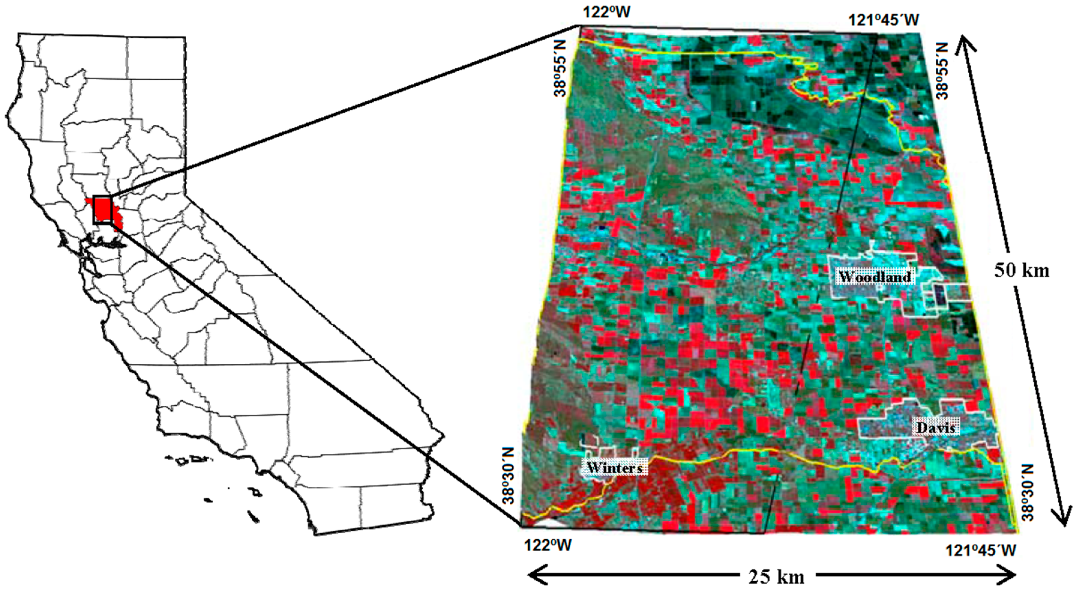
2.1. Study Area Description

The investigation was carried out in the cropland area located in Yolo County (California, USA), with center coordinates 38.5°N and 121.5°W (Datum NAD83) (Figure 1). This region has a Mediterranean climate, characterized by hot, dry summers (daily maximum temperatures over 38 °C) and cool winters (daily maximum temperatures of 16 °C). Rainfall ranges from 200 mm to 460 mm, and occurs mostly from November through March, so crops growing in the summer are generally irrigated. Soils are mostly deep, as is common in the rich alluvial plains of the Sacramento River. A high consumption of water resources is demanded in the summer; so, determining the crop-growing events (e.g., dates of vegetation green-up and senescence) in this season has strong implications in the management of irrigated land. Yolo County has a total agricultural surface of 177,000 ha, plus 87,900 ha occupied by dry meadows and other land uses. In order to balance between study diversity and complexity, our study focused on seven major crops grown in the summer season, as follows: tomato (14% of Yolo County cropland surface), rice (10%), sunflower (6%), and maize (4%) as herbaceous crops, and walnut (5%), vineyard (4%), and almond (3%) as deciduous woody crops. These crops cover about 50% of the cropland surface, among a total of as many as 130 different commodities [29].

2.2. Satellite Imagery
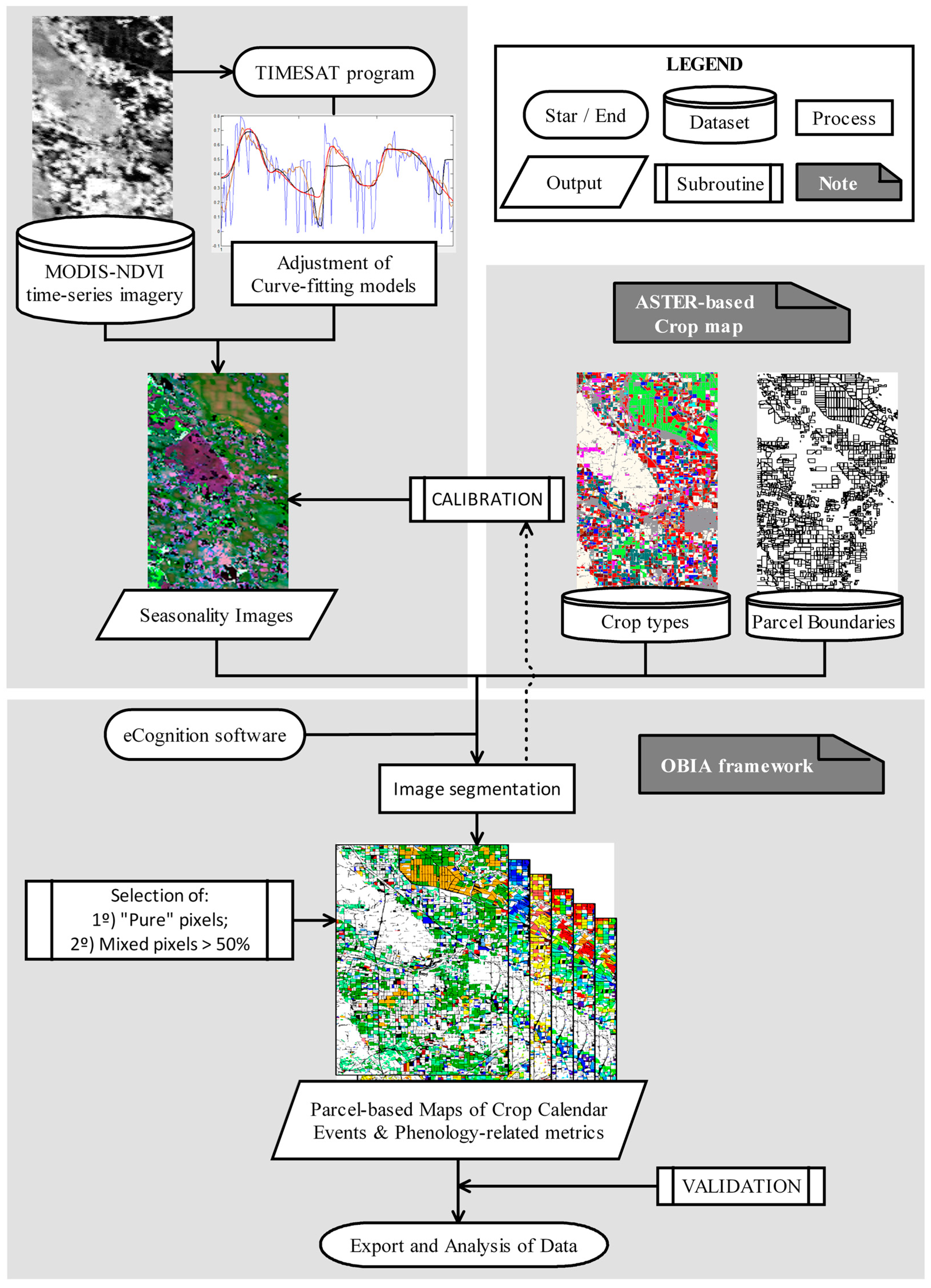
A set of daily MODIS satellite images at a 250-m resolution (product MOD09GQ, version 6) provided by NASA’s Earth Observing System during three consecutive years (2005, 2006 and 2007) were used in this investigation. These MODIS products were provided with correction for atmospheric gases and aerosols, quality assurance (QA) data layers, and surface spectral reflectance values in the red (620–670 nm) and infrared (841–876 nm) bands to calculate the NDVI time-series used for deriving vegetative development. QA information allowed to identify cloud coverage, solar zenith angle, and other noise on the pixels and correct these anomalies. Remaining disturbance that could affect NDVI data quality was later filtered out with the application of the curve-fitting models and a spike removal procedure (see Section 2.3.1). Of the three study years, our analysis focused on the central year (2006), while the MODIS data of the adjacent years were additionally used to maintain data continuity at the extremes of the central year and ensure that the models fit over the entire season. Therefore, in the event that only data for the target year are available, an operational solution would be to spill over such data to the adjacent years, thus solving this particular condition [12].
We selected this specific cropland area and the year 2006 as the target year because an accurate crop map and reliable ground-truth crop data of the study region in that year were available, which enabled supporting the results from detailed calibration/validation data composed of 350 crop parcels (see Section 2.4). The crop map was previously obtained in a parallel study [27] by classifying three Advanced Spaceborne Thermal Emission and Reflection Radiometer (ASTER) satellite images taken in the mid-spring, early summer, and late summer of 2006 (see Section 2.3.2). Both MODIS and ASTER sensors are onboard the same NASA EOS Terra satellite platform, so a MODIS-NDVI time-series and an ASTER-based crop map were derived from observations obtained at the same height and coincident nadir. Both types of images have a geolocation accuracy of lower than 50 ± 15 m [30], so potential co-registration errors can be considered negligible at the spatial scale of this investigation.

2.3. Methodology

The full procedure comprised three interrelated parts (Figure 2): (1) the generation of seasonality images by adjusting curve-fitting models to a MODIS-NDVI time-series; (2) the segmentation and identification of crop parcels using the ASTER-based crop map and calibration of crop-specific models; and (3) the generation of parcel-based maps of crop calendar events and phenology-related metrics in an OBIA framework. Part 1 was implemented with TIMESAT computer software developed by Jönsson et al. [12], and parts 2 and 3 were implemented with the eCognition Developer software (Trimble GeoSpatial, Munich, Germany). The methodology that was used in each part is detailed as follows.

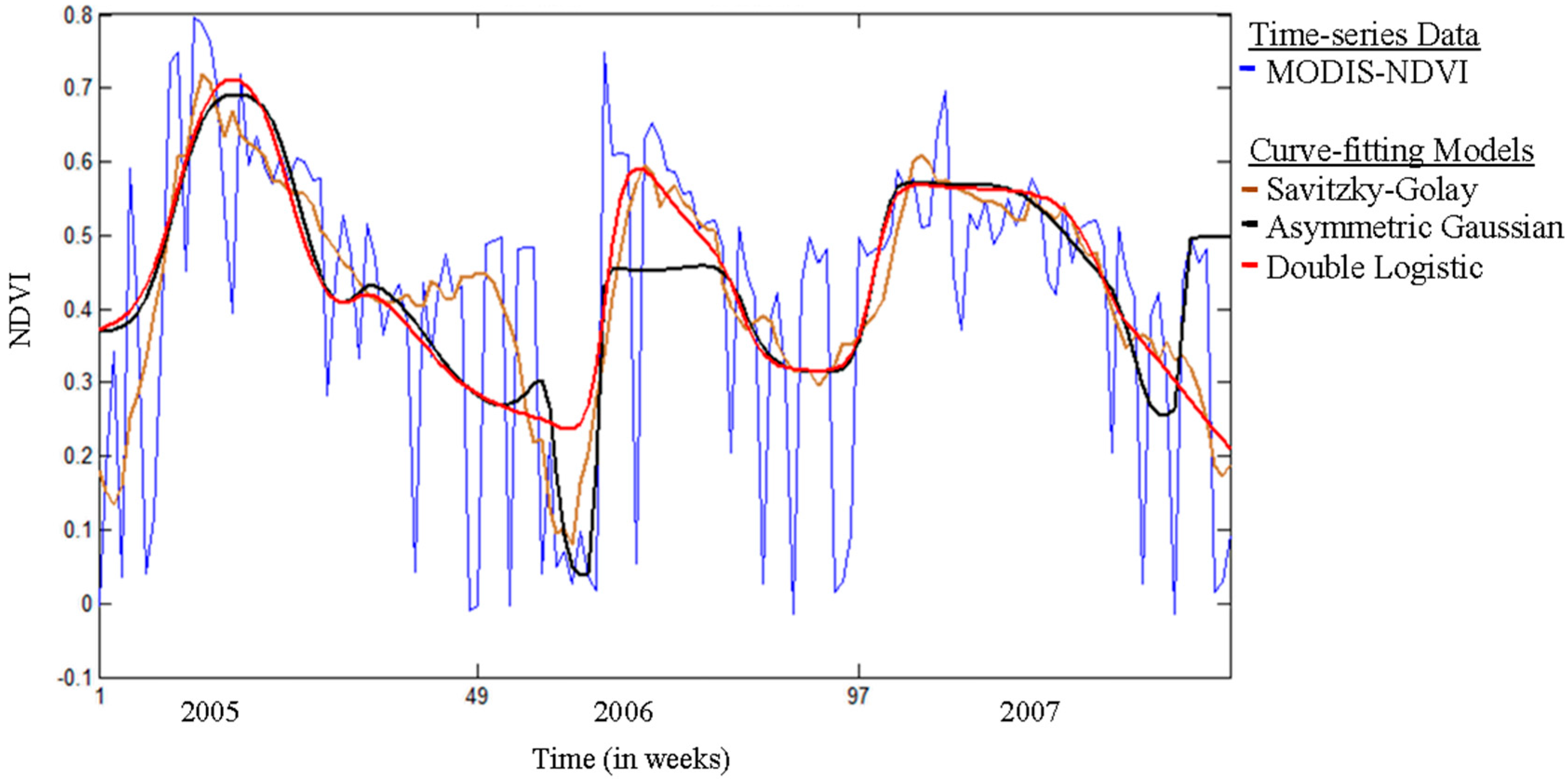
2.3.1. Part 1: Generation of Seasonality Images by Adjusting Curve-Fitting Models to the MODIS-NDVI Time-Series

TIMESAT consists of a number of numerical and graphical routines coded in Matlab and Fortran, which were developed to generate several crop seasonality images by fitting a smooth model function to the upper envelope of remotely sensed time-series data [10]. In this investigation, we evaluated the three different curve-fitting models implemented in TIMESAT, named Savitzky–Golay (SG) filtering, asymmetric Gaussian (AG), and double logistic (DL) (Figure 3), as well as several configurations according to a number of specific input settings, as follows: (1) number of interannual growing seasons; (2) distribution of data weight; (3) method for removal of spikes and outliers; (4) number of envelope iterations; (5) adaptation strength; and (6) size of the moving window (only in SG filtering). The seasonality images that produced each model changed according to the combination of these settings, so the optimal configuration of each model as affected by the crop types was determined in a calibration phase (see Section 3.1).
Once the best curve-fitting model and their optimal settings were defined for each studied crop (calibration phase), we applied these crop-specific models to process MODIS-NDVI time-series data for pixels of the entire study region, and generated a number of images of the 11 seasonality variables provided by TIMESAT (Figure 4). The parameters Start, End, Middle and Length of the Season are indicators of crop calendar events, estimating the dates and timing in which each parcel was covered by the crop; otherwise, it was uncultivated or was bare soil. According to Eklundh et al. [31], these four crop calendar events were calculated as follows. (1) The Start of the Season is the point in time for which the left edge of the fitted function has increased to a certain number; it is defined by the user, and measured between the left minimum level and the maximum. (2) The End of the Season is the point in time for which the right edge of the fitted function has decreased to a user-defined level measured from the maximum to the right minimum level. (3) The Middle of the Season is the time computed as the mean of the times for which, respectively, the left edge of the fitted function has increased to the 80% level, and the right edge has decreased to the 80% level. (4) Last, the Length of the Season is the time from the start to the end of the season.
In addition to the crop calendar events, the parameters Base, Maximum, Amplitude, Left Derivative, and Right Derivative, and Large Integral, and Small Integral are indicators of crop dynamics, having been related to variations on crop phenology, vegetation vigor, and crop productivity [32,33,34]. According to Eklundh et al. [31], these seven phenology-related metrics were calculated as follows (Figure 4). (1) The Base is the average of the left and right minimum NDVI values of the fitted function. (2) The Maximum is the largest NDVI value of the fitted function during the season. (3) The Amplitude is the difference between the maximum and the base values. (4) The Left Derivative is the ratio of the difference between the left 20% and 80% levels of the fitted function and the corresponding time difference. (5) The Right Derivative is the absolute value of the ratio of the difference between the right 20% and 80% levels of the fitted function and the corresponding time difference. (6) The Large Integral is the area between the fitted function and the zero level. (7) Lastly, the Small Integral is the area between the fitted function and the base value.

2.3.2. Part 2: Segmentation and Identification of Crop Parcels Using the ASTER-Based Crop Map and Calibration of Crop-Specific Models

The crop map is a vector file with georeferenced information of the boundaries and the type of crop of each parcel in the study region, which was previously created in Peña-Barragán et al. [27] by implementing the Object-based Crop and Identification Mapping (OCIM) methodology. OCIM consisted of a decision tree algorithm of several vegetation indices and textural features derived from the ASTER green, red, near-infrared (NIR), and short-wave infrared (SWIR) bands registered in three dates that are crucial for crop classification, i.e., in the mid-spring (7 May), early summer (24 June), and late summer (12 September). The OCIM output was a map of 15-m spatial resolution (ASTER maximum resolution) with several classes including urban/road, meadow lands, and 12 different crops, although we only selected the major herbaceous (corn, rice, sunflower, and tomato) and woody (almond, vineyard, and walnut) crops with annual growth cycles for the crop map used in this investigation. The crop map was evaluated in Peña-Barragán et al. [27] by using an independent ground-truth (GT) dataset of 350 crop fields, which reported user’s and producer’s accuracies of 83% and 81% on average, respectively. The crop map was used in this research as a thematic layer to segment the parcels in the seasonality images generated by TIMESAT and label the crop type of each of these parcels, which resulted in an OBIA framework of TIMESAT-based images at the ASTER maximum spatial resolution (i.e., 15 m).
At this point, a calibration phase was performed to select the best configuration of each curve-fitting model from a pool of 288 seasonality images created with all of the possible combinations of parameters indicated in Table 1, and using 110 calibration parcels (see Section 2.4). A unique interannual growing season was considered in all of the parcels, and the same weights were assigned to original data prior to the application of the spike removal method. Then, two different methods for removing spikes and outliers were tested and compared to no-spike detection, as follows. (1) The first was the media filtering method, in which values substantially different from both the left and right-hand neighbors and from the median in a window are classified as outliers. (2) The seasonal-trend decomposition procedure based on loess (STL-decomposition) method was the second method, in which the full time-series is divided into a seasonal and a trend component, and data values that do not fit this pattern are assigned low weights [35]. Additionally, three envelope iterations, four values of adaptation strength, and, in the case of the SG filtering, two sizes of the moving window were also evaluated. The term “envelope iterations” refers to the number of fits (one, two, or three) used by the function to approach the upper envelope of the time-series in an iterative procedure. The adaptation strength indicates the strength of the upper envelope adaptation, ranging from a maximum of 10 (the strongest adaptation to the upper envelope) and a minimum of 1 (no adaptation). Finally, the size of the moving window in the SG filtering determines the degree of smoothing, but it also affects the ability to follow a rapid change. For a detailed description of the mathematical base of the models and their settings, readers can refer to Lumbierres et al. [32].

2.3.3. Part 3: Parcel-Based Mapping of Crop Calendar Events and Phenology-Related Metrics

The OBIA procedure used the full dataset composed of the ASTER-based crop map and of 11xN TIMESAT-based seasonality images, with N being the number of crop-specific models selected in the calibration phase (see Section 2.3.1). First, all of the seasonality images were segmented according to the ASTER-based crop map and, as a result of this segmentation, the OBIA procedure automatically assigned to every object (crop-parcel) its value of crop type (from the crop map) and an averaged value of each seasonality variable (11xN values). To mitigate the impact of mixed pixels, the OBIA procedure was designed to automatically apply a restrictive criterion based on the coverage of MODIS-NDVI pixels in each parcel: (1) using only MODIS-NDVI pixels that are 100% within each crop parcel (i.e., “pure” pixels); or (2) if no “pure” pixels exist in any parcel, using only pixels with coverage percentages greater than 50% and, in such a case, reporting the mixing percentage in the output file. Next, an automatic if–then algorithm linked the correct seasonality image to every parcel according to its crop type (part 1) and to its crop-specific model selected in the calibration phase (part 2). For example, if the best curve-fitting model for the crop rice was model-A and for walnut it was model-B, then the algorithm will only use the seasonality images derived from model-A in the rice parcels and from model-B in the walnut parcels. Finally, parcel-based maps of the four crop calendar events and of the seven phenology-related metrics were created according to the crop growing in each parcel.

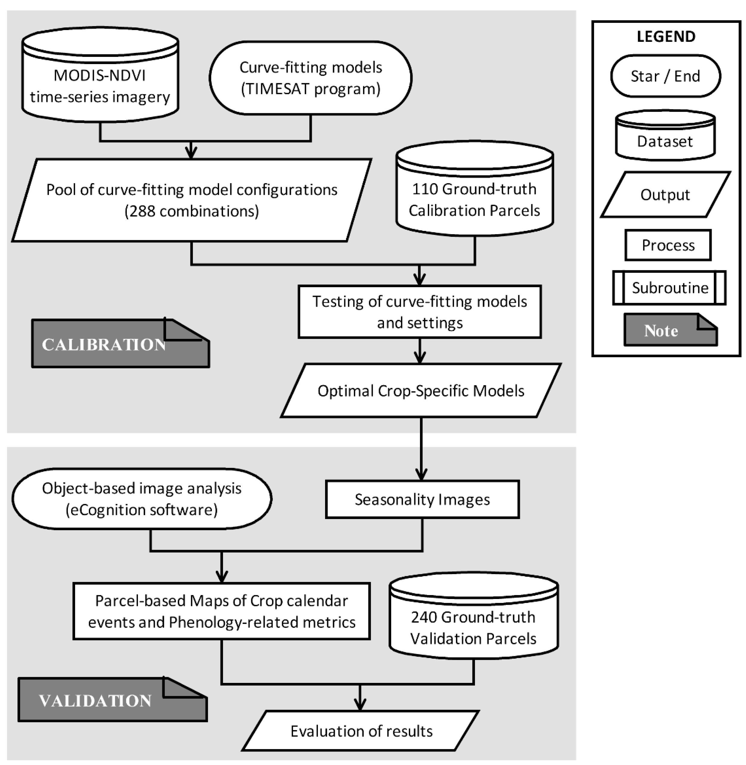
2.4. Calibration and Validation of the Methodology

We conducted a calibration/validation approach to optimize the curve-fitting models and evaluate the performance of the full OBIA procedure (Figure 5). For this purpose, 30 parcels of corn, 40 parcels of almond and vineyard, and 60 parcels of rice, sunflower, tomato, and walnut (350 parcels in total) were randomly selected throughout the studied region, representing around 6% of the Yolo County agricultural area. The type of crop and key calendar dates (i.e., start and end of the season) in each field were confirmed from maps provided by the Yolo agricultural commissioner’s office and double-checked by frequent field surveys. In the case of herbaceous crops, the start and end of the season were defined as the crop emergence date and the harvest date, respectively. For woody crops, the season started after the dormancy period, which corresponded to bud break and leaf growth, while the season ended after senescence and leaf fall.
The size of the calibration and validation dataset was approximately n/3 and 2n/3, respectively, with n being the size of the full dataset (n = 350). The calibration phase consisted of testing 288 different model configurations derived from combining the settings listed in Table 1. Estimations of crop calendar events (start and end of season) from each output of the tested models were compared to the data that were observed in 110 calibration ground-truth fields, which reported the optimal model and its settings for each studied crop (see Section 3.1). Next, we used the models selected for each crop type to map the crop calendar events and the phenology-related metrics in the OBIA framework (see Section 3.2). Finally, the full procedure was validated with 240 independent ground-truth crop parcels by quantifying the number of parcels whose estimated and observed crop calendar events were within a range of two weeks.

3. Results

3.1. Configuration of the Curve-Fitting Models as Affected by the Type of Crop

The three models implemented in TIMESAT varied significantly according to the range of values given to the several settings listed in Table 1. In order to select the best configuration for each model and crop type, all of the possible setting combinations were iteratively tested in a first phase applied to the time-series data of 110 calibration parcels. A logical criterion for model selection is minimizing the root mean square error (RMSE) between the values estimated model and the values observed in the MODIS-NDVI time-series data, i.e., the smaller the RMSE, the better is the model adjustment [36,37]. However, this measure is biased by the observed data, so it can provide a low averaged RMSE, but imprecise estimations of the crop calendar events in case of incomplete or noisy MODIS-NDVI values in the season extremes. As an alternative criterion, following the objectives of this investigation, the models were configured according to the minimum differences between the estimated and observed start and end days of the season. Table 2 shows a ranking of models and their optimal settings selected for each type of crop. To our knowledge, details on model configurations have not been reported in previous investigations on crop phenology.
The performance of the SG filtering was superior in most crops, with the exception of rice, while the performance of the AG model was intermediate in all of the cases. In terms of fitting the start of the season, the SG model provided high accuracy for corn, rice, tomato, and almond (three to six days of averaged error), and moderate adjustment for sunflower, vineyard, and walnut (nine to 16 days of averaged error), while the AG and the DL models performed the worst in all of the cases (seven to 30 days of averaged error). Regarding the end of the season, the SG filtering adjusted better than the other models for corn, sunflower, tomato, vineyard, and walnut (six to 12 days of averaged error), but adjusted the worst for rice and almond (13–17 days of averaged error). In these two crops, the DL model obtained the best adjustment (6–16 days of averaged error). By group of crops, the model adjustments of the herbaceous crops were generally more accurate than the woody crops, although the three models fitted to walnut slightly better than to sunflower. It was also observed that the SG model adjusted better to the start of the season in the herbaceous crops and almond, and to the end of the season in vineyard and walnut. However, the AG and DL models adjusted better to the end of the season in all of the crops, with the exception of the AG model in almond.
Although the range of setting values tested in this investigation was diverse, the optimal configurations were mostly similar in the three models and the seven crops (Table 2). A range of NDVI values between −1 and 1 was specified for all of the cases, which implies that all of the potential NDVI values were used for model adjustment. The no-spike method was the best option in six crops, with the exception of rice, which preferred the media filtering method to remove spikes and outliers. On the contrary, the STL-decomposition spike-removal method was not selected in any case. The SG and DL models produced the best adjustment for all of the crops with two envelope iterations and with no adaptation to the upper envelope (adaptation strength value of one), while the AG model fitted to the upper envelope of the time-series data with only one iteration in corn, tomato, and walnut, and with two iterations in the rest of crops, as well as with a smooth adaptation strength (value of three) to the upper envelope for all of the cases. Finally, between the two different sizes of the moving window tested in the SG filtering, the highest degree of smoothing (value of 10) was chosen for all crops studied.

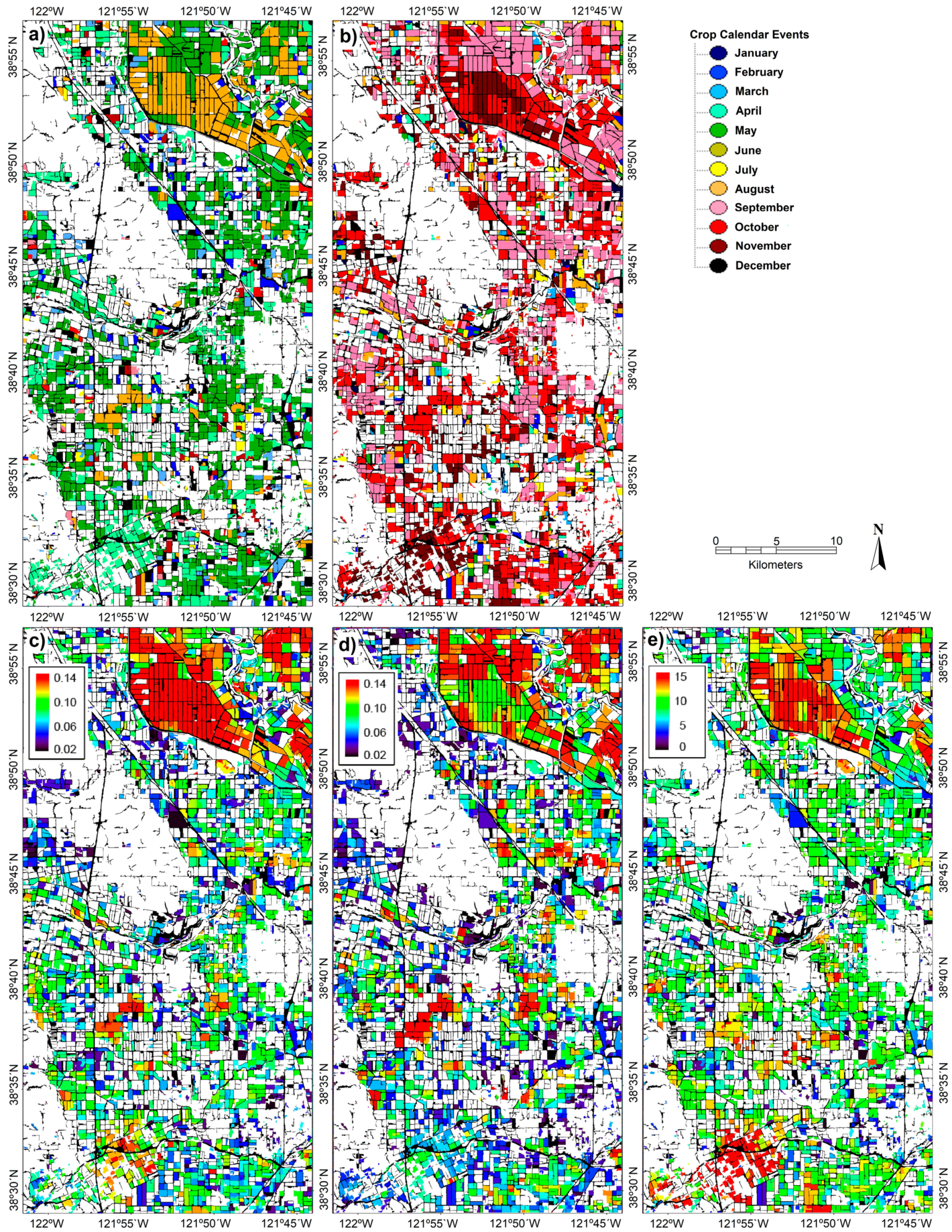
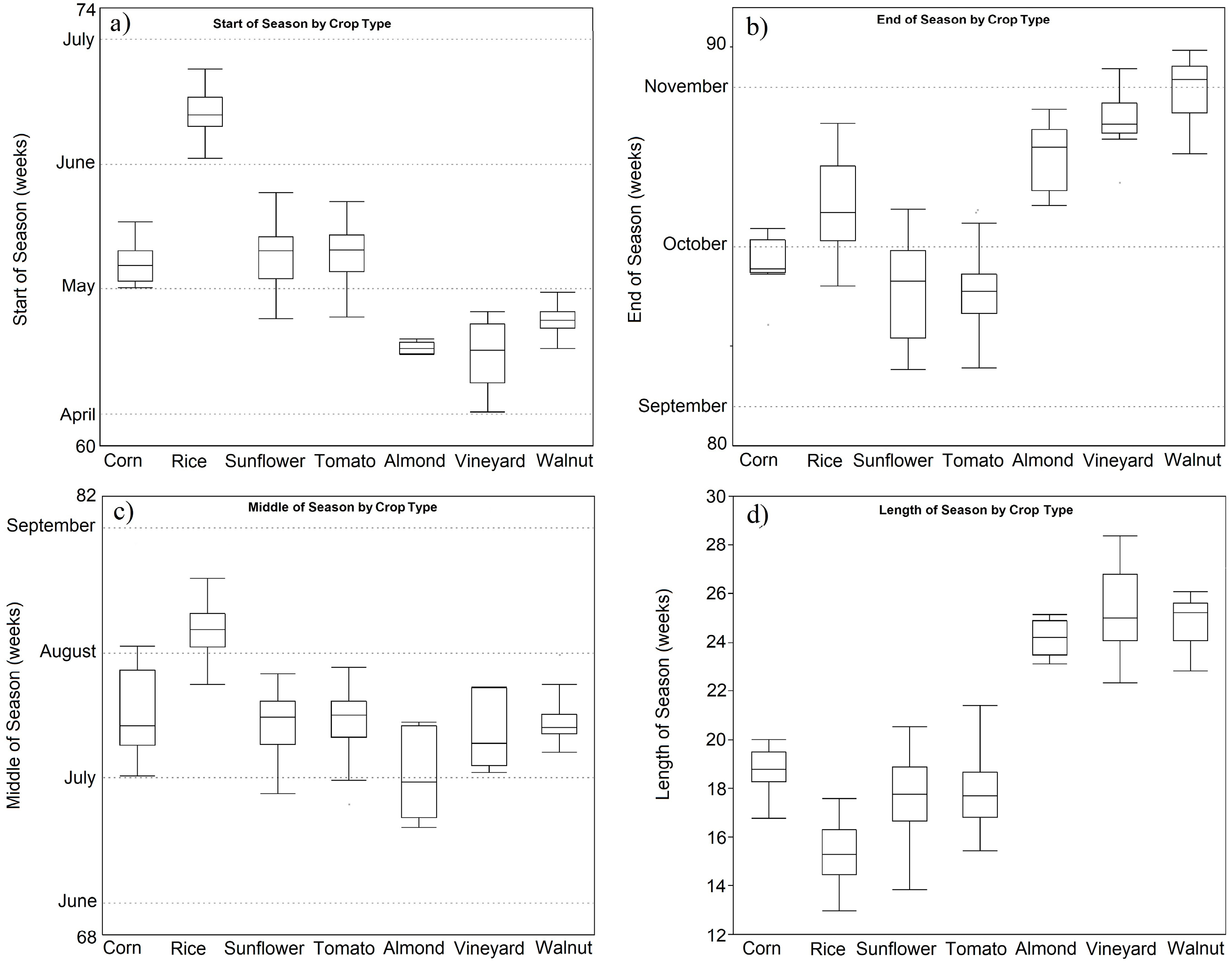
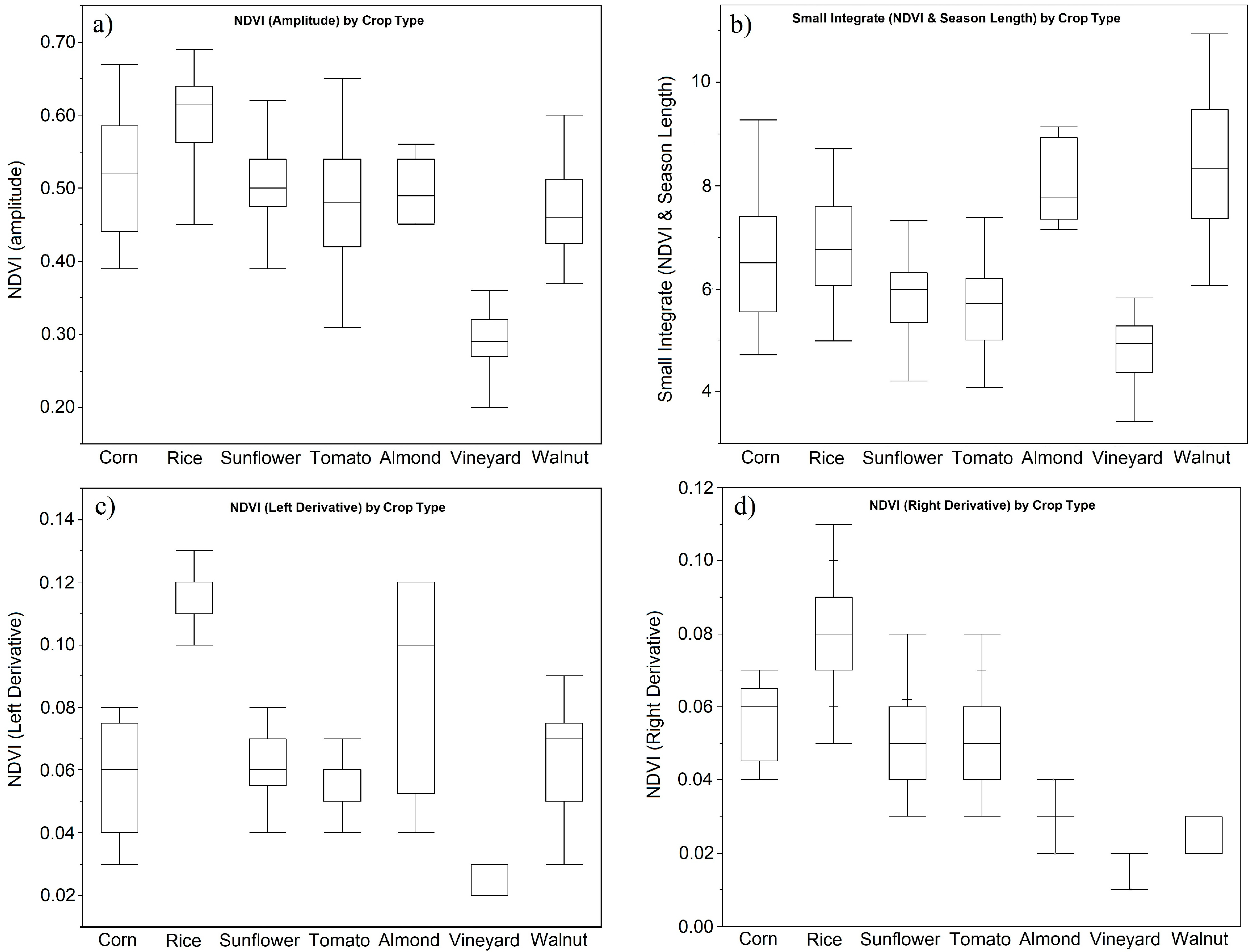
3.2. Maps of Crop-Calendar Events and Phenology-Related Metrics

After the preliminary phases of image segmentation and classification, the OBIA procedure automatically applied the curve-fitting model that better adjusted to each type of crop (selected in Table 2) and produced several maps with detailed information on the level of individual parcels (Figure 6). As a result of using an object-based framework, numerous metrics of every parcel and statistics of the study region were computed and then exported in various formats of image raster (e.g., TIFF, jpg), vector (e.g., shapefile), and table (e.g., csv or txt) files for further analysis. This is a valuable innovation that was not available in past research on crop phenology, which applied conventional pixel-based methods. Table 3 illustrates a partial view of the database reported in our case study, which is summarized into three blocks: (1) general data of every parcel, including geographic location, parcel size, and crop type; (2) crop calendar events; and (3) phenology-related metrics.
The Start of Season and End of Season maps (Figure 6a,b, respectively) were used to evaluate the performance of the full procedure by direct comparison of the map values against real crop calendar measures observed in 240 independent parcels of validation. The rest of the maps were not validated, because capturing on-ground measurements of phenology-related metrics was not feasible at the spatial coverage of the entire study region, as also noted by Jamali et al., Tan et al. [14,38]. Table 4 counted the number of parcels in which the estimated and observed dates were within a range of two weeks. This validation range is reasonable, given the diversity of crop varieties and farming strategies observed in the study region, which made it difficult to establish the exact calendar dates from on-ground field observations. According to this criterion, the dates of the Start of Season were correctly estimated from a minimum value of 70% of the vineyard parcels to a maximum value of 100% of the almond parcels, although most of the crops attained accuracies greater than 85%. However, the results in estimating the dates of the End of Season were most accurate in the vineyard parcels (97%) and least accurate in the almond parcels (57%), which might imply some degree of mismatching of the curve-fitting model selected in these two crops (i.e., Savitzky–Golay filtering in both cases). In total, the dates of the Start and End of Season were correctly estimated in 213 and 196 cases, which consisted of 89% and 82% of the validation fields, respectively.
Detailed analysis of the maps (e.g., Figure 6) and tables (e.g., Table 3) derived from our procedure revealed significant differences in the phenology of some major crops growing in the entire study region. Regarding crop calendar events (Figure 7), permanent woody crops (i.e., almond, walnut, and vineyard) showed earlier dates of Start of Season (mid-April on average) and later dates of End of Season (from mid-October to early November on average) in comparison to annual herbaceous crops (i.e., corn, rice, sunflower, and tomato), in which the crop cycle started about early May and ended about late September in most cases (Figure 7a,b, respectively). However, the green-up date of the flooded rice fields was generally much later than the rest of the herbaceous crops, since these fields were covered by water in early crop growth stages, and this interfered with the estimations from the temporal MODIS-NDVI profiles for about 30–40 days until the rice canopy was closed, as also indicated by Dong et al. [21]. The interval between the beginning and end of the season (i.e., Length of Season) is critical in summer crops for scheduling irrigation, while the Middle of Season identifies the period in which the demand of the crops for water generally reaches maximum levels [39]. On the one hand, the mid-season of most of the crops in our study was about July on average, although many almond fields brought this date forward to the end of June, and many rice fields delayed it to early September (Figure 7c). On the other hand, the Length of Season values that were estimated for the herbaceous crops ranged between 15–16 weeks in the rice parcels and 18–19 weeks in the corn fields, and for the woody crops, these were about 24–26 weeks in the three studied crops (Figure 7d). This was consistent with the typical crop calendar patterns as described in the study region [40].
With respect to the phenology-related metrics, boxplots of value distribution revealed different patterns of crop development as indicated by the annual NDVI variation of each studied crop (Figure 8). In the study region, the NDVI Amplitude was in an average range of 0.40 to 0.65 in most of the crops, with the exception of many vineyard parcels that reached much lower amplitude (about 0.30 on average) (Figure 8a). Higher differences of NDVI Integral were observed between herbaceous and woody crops (Figure 8b). The highest values were reported in the almond and walnut parcels, and the lowest values were reported in the vineyard parcels, while the herbaceous crops reached intermediate values in this descending order: rice, corn, sunflower, and tomato. According to the NDVI Left Derivative, rice and almond generally grew faster than the other crops, and vineyard was the slowest in most cases (Figure 8c), while the NDVI Right Derivative showed that herbaceous crops ripened faster than woody crops, with the NDVI values of the rice and vineyard parcels being respectively the fastest and the slowest ones to fall during the senescence stages, respectively (Figure 8d).

4. Discussion

Several procedural aspects (curve-fitting modeling, MODIS data quality, spatial and temporal resolution) and agro-ecological implications can be derived from this research. Of the three models explored, the best performance of the adaptative SG filtering in most crops might be attributed to this model using local polynomial functions to smooth time-series data, replacing each data by a linear combination of nearby values in a moving window. Therefore, it can fit subtle fluctuations in the data and suppress certain disturbances. In addition, the process of selecting the optimal model parameters is considered an advantage for local filtering (i.e., SG filtering in this study) in comparison to the other methods [5]. However, the SG filtering is also the most sensitive to noise among the three methods [38]. This might justify its worst adjustment in rice, which was perhaps due to the sun-glitter effects in the spectral response of the typically flooded parcels of this crop [41], although no clear evidence of this effect was observed when examining the QA information on sun glint (icm_sun_glint). On the other hand, the AG and DL methods are semi-local non-linear functions that fit to time-series data in intervals around its maximum and minimum, being well suitable for describing the shape of the time-series data in overlapping intervals around data extremes. According to Gao et al. [42], these two model functions are very similar in performance, although the AG method works better with incomplete time-series data, which is an important advantage in case the studied satellite has missing data. Previous investigations in relation to the implementation of curve-fitting models in vegetation scenarios reported divergent conclusions, which demonstrate the complexity of proposing a universal and robust methodology [5,43]. While Beck et al. [37] highlighted the DL model and Tan et al., Gao et al. [38,42] highlighted the AG model in comparison to other methods, Hird et al., Atkinson et al. [11,36] found that both models have similar performance and are superior to SG filtering in the monitoring of natural vegetation. On the contrary, in agricultural scenarios where annual crops represent the most extensive area, the SG filtering produced better results [44], which is in agreement with the result of this investigation.
In this research, the MOD09GQ product was selected among the many MODIS products available [45], as a balance between its higher temporal resolution (daily frequency) and the moderate quality of its original data. An alternative used in several previous investigations is the MOD09Q1 images [15,19], which are eight-day composites of MOD09GQ selected on the basis of high observation coverage, low view angle, the absence of clouds or cloud shadow, and aerosol loading. Both products have similar spatial resolution (250 m), but they differ in temporal resolution, which is crucial for monitoring vegetation conditions. Alexandridis et al. [46] studied the issue of appropriate temporal sampling for vegetation, and concluded that a seven-day period is the optimum time step for managed crops, which is near the eight-day composites of MOD09Q1. However, MODIS composites do not always provide data in the expected range (i.e., eight consecutive days), as the period can vary between extreme dates of consecutive composites, and therefore be separated by up to 14 days [47]. In this context, it should be considered that, as demonstrated in this paper and in recent studies [2,18], it is now possible to study MODIS data at the parcel level by using an OBIA framework, so very frequent observation is recommended in order to detect small differences in the NDVI profiles of crops with similar phenology.
The maps developed in this investigation provided valuable information on crop phenology and land-use changes (i.e., soil is bare or is covered by any crop or residue, for how long, which crop is growing, etc.) in every specific parcel over time, which has applications to improve the tasks of crop identification and monitor vegetation trends and agricultural activities [14,15,23,26], and is very relevant for agro-ecological studies. For instance, the amplitude of NDVI (i.e., increase between baseline and maximum NDVI values) and, to a greater extent, the integrals of NDVI (i.e., cumulative NDVI values over crop development) are measurements of crop vigor, and have been considered as predictors of plant or tree biomass productivity [32,34], net primary production [33,48], and crop yield [49]. In addition, the slopes of NDVI increase and NDVI decrease during the beginning and the ending of the season (i.e., NDVI Left Derivative and NDVI Right Derivative, respectively) might indicate the speeds at which the crop is growing after emergence and is ripening prior to harvest, respectively [10,33]. This information can also assist the decision-making processes of agrarian policy actions related to water supply and drought monitoring [50,51,52], food security [15], crop growing, and yield assessment [49], or the implementation of certain agro-environmental measures [53]. In addition, these remote-sensed products may be integrated with ecosystem models in order to assess greenhouse gas (GHG) cycling from agricultural crops at the regional scale and decrease the uncertainty in estimations of such models [54,55]. Although many ecosystem models have been successfully validated at the field level, a comprehensive assessment of GHG (especially CO2 and NH4 fluxes) across multiple spatial and temporal scales in agro-ecosystems is still challenging [56]. Therefore, the incorporation of remotely-sensed datasets containing crop calendar events and phenology-related metrics combined with additional field information and modeling runs will allow extrapolating field-site estimations of GHG fluxes to county and regional scales, which is going to be essential to assess how alternative strategies on cropland management can play a potential role in GHG mitigation options for agriculture.

5. Conclusions

Past research on monitoring crop phenology with remote sensing was limited to scenarios with few land uses or crop types that usually cover areas larger than real parcel sizes. The procedure presented here goes beyond these limitations, and extends its application to a cropland region with diverse crops (i.e., corn, rice, sunflower, and tomato as herbaceous crops, and almond, vineyard, and walnut as woody crops) and to the level of individual crop parcels, in which several parcel-based maps with crop phenology information were produced by adjusting curve-fitting models to MODIS-NDVI time-series imagery in an OBIA framework.
A first calibration phase evaluated the three curve-fitting models implemented in the TIMESAT software and selected Savitzky–Golay filtering as the best model in most crops, with the exception of the Double Logistic model, which was better in rice. The asymmetric Gaussian model was intermediate in all of the cases. After testing 288 different model configurations, we concluded that the optimal settings were very similar in the three curve-fitting models for the seven studied crops. However, our results partially differed from other investigations that have been developed in diverse vegetation scenarios, which demonstrated the complexity of proposing a unique solution; so, calibration of the curve-fitting models is recommended to extrapolate this method to other study regions.
After applying the crop-specific models to the MODIS-NDVI time-series of the entire region, the OBIA procedure generated the maps of crop calendar events (i.e., start, end, middle, and length of the season) and phenology-related metrics (i.e., base, maximum, amplitude, derivatives, and integrals of the NDVI values) of every crop parcel with an overall accuracy of 89% and 82% in the estimation of the dates of start and end of the season, respectively, which confirmed the reliability of these maps. A detailed analysis of these maps revealed some differences between the studied crops, e.g., the length of the season ranged between 15–16 weeks in the rice parcels, 18–19 weeks in the corn fields, and 24–26 weeks in the woody crops, the NDVI Integral (which is related to crop vigor and productivity) was maximum in the almond and walnut parcels and minimum in the vineyard parcels, and the NDVI Left Derivative and NDVI Right Derivative (which are related to the speeds of crop growing and ripening, respectively) showing that the crops generally grew faster in the rice and almond parcels and slower in the vineyard parcels, while the herbaceous crops ripened faster than the woody crops, respectively.
Our innovative procedure demonstrated the capability of remote sensing technology to monitor crop phenology not only over extensive areas but also at the level of individual crop parcels by applying an OBIA framework, providing valuable geospatial information as input data for several agro-environmental applications in cropland management, irrigation scheduling, or ecosystem modeling. Although the procedure was developed with the specific characteristics of a case study located in central California, we consider that its general scheme is universal and its main settings are customizable, enabling its application to other cropland regions after applying the phases of calibration and validation described here.

Author Contributions

Conceptualization, J.S., R.E.P. and J.M.P.; Methodology, A.I.C. and J.M.P.; Software, A.I.C.; Validation, A.I.C. and J.M.P.; Formal Analysis, A.I.C. and J.M.P.; Investigation, All authors; Resources, J.S., R.E.P. and J.M.P.; Data Curation, A.I.C. and J.M.P.; Writing-Original Draft Preparation, A.I.C. and J.M.P.; Writing-Review & Editing, All authors; Visualization, A.I.C. and J.M.P.; Supervision, R.E.P. and J.M.P.; Project Administration, J.S. and J.M.P; Funding Acquisition, J.S. and J.M.P.

Funding

This research was funded by the Kearney Foundation of Soil Science (Davis, CA, USA) and the AGL2017-83325-C4-1-R project (Spanish Ministry of Economy, Industry and Competitiveness—MINECO and EU-FEDER funds). MODIS data were available to us through a NASA EOS scientific investigator affiliation. Research of Ana I de Castro and José M Peña was financed by the “Juan de la Cierva” and “Ramón y Cajal” (grant ref. RYC-2013-14874) Programs (MINECO funds), respectively.

Acknowledgments

We acknowledge support of the publication fee by the CSIC Open Access Publication Support Initiative through its Unit of Information Resources for Research (URICI).

Conflicts of Interest

The authors declare no conflict of interest.

References

  1. Chen, B.; Huang, B.; Xu, B. Multi-source remotely sensed data fusion for improving land cover classification. ISPRS J. Photogramm. Remote Sens. 2017, 124, 27–39. [Google Scholar] [CrossRef]
  2. Gao, F.; Anderson, M.C.; Zhang, X.; Yang, Z.; Alfieri, J.G.; Kustas, W.P.; Mueller, R.; Johnson, D.M.; Prueger, J.H. Toward mapping crop progress at field scales through fusion of Landsat and MODIS imagery. Remote Sens. Environ. 2017, 188, 9–25. [Google Scholar] [CrossRef]
  3. Verstraete, M.M.; Gobron, N.; Aussedat, O.; Robustelli, M.; Pinty, B.; Widlowski, J.-L.; Taberner, M. An automatic procedure to identify key vegetation phenology events using the JRC-FAPAR products. Adv. Space Res. 2008, 41, 1773–1783. [Google Scholar] [CrossRef]
  4. Zhang, X.; Friedl, M.A.; Schaaf, C.B.; Strahler, A.H.; Hodges, J.C.F.; Gao, F.; Reed, B.C.; Huete, A. Monitoring vegetation phenology using MODIS. Remote Sens. Environ. 2003, 84, 471–475. [Google Scholar] [CrossRef]
  5. Cai, Z.; Jönsson, P.; Jin, H.; Eklundh, L. Performance of Smoothing Methods for Reconstructing NDVI Time-Series and Estimating Vegetation Phenology from MODIS Data. Remote Sens. 2017, 9, 1271. [Google Scholar] [CrossRef]
  6. Chandola, V.; Hui, D.; Gu, L.; Bhaduri, B.; Vatsavai, R.R. Using Time Series Segmentation for Deriving Vegetation Phenology Indices from MODIS NDVI Data. In Proceedings of the 2010 IEEE International Conference on Data Mining Workshops, Sydney, Australia, 13 December 2010; pp. 202–208. [Google Scholar]
  7. Colditz, R.R.; Conrad, C.; Wehrmann, T.; Schmidt, M.; Dech, S. TiSeG: A Flexible Software Tool for Time-Series Generation of MODIS Data Utilizing the Quality Assessment Science Data Set. IEEE Trans. Geosci. Remote Sens. 2008, 46, 3296–3308. [Google Scholar] [CrossRef]
  8. Roerink, G.J.; Menenti, M.; Verhoef, W. Reconstructing cloudfree NDVI composites using Fourier analysis of time series. Int. J. Remote Sens. 2000, 21, 1911–1917. [Google Scholar] [CrossRef]
  9. Udelhoven, T. TimeStats: A Software Tool for the Retrieval of Temporal Patterns from Global Satellite Archives. IEEE J. Sel. Top. Appl. Earth Obs. Remote Sens. 2011, 4, 310–317. [Google Scholar] [CrossRef]
  10. Jönsson, P.; Eklundh, L. TIMESAT—A program for analyzing time-series of satellite sensor data. Comput. Geosci. 2004, 30, 833–845. [Google Scholar] [CrossRef]
  11. Hird, J.N.; McDermid, G.J. Noise reduction of NDVI time series: An empirical comparison of selected techniques. Remote Sens. Environ. 2009, 113, 248–258. [Google Scholar] [CrossRef]
  12. Jönsson, P.; Eklundh, L. Seasonality extraction by function fitting to time-series of satellite sensor data. IEEE Trans. Geosci. Remote Sens. 2002, 40, 1824–1832. [Google Scholar] [CrossRef]
  13. Bradley, B.A.; Jacob, R.W.; Hermance, J.F.; Mustard, J.F. A curve fitting procedure to derive inter-annual phenologies from time series of noisy satellite NDVI data. Remote Sens. Environ. 2007, 106, 137–145. [Google Scholar] [CrossRef]
  14. Jamali, S.; Jönsson, P.; Eklundh, L.; Ardö, J.; Seaquist, J. Detecting changes in vegetation trends using time series segmentation. Remote Sens. Environ. 2015, 156, 182–195. [Google Scholar] [CrossRef] [Green Version]
  15. Massey, R.; Sankey, T.T.; Congalton, R.G.; Yadav, K.; Thenkabail, P.S.; Ozdogan, M.; Sánchez Meador, A.J. MODIS phenology-derived, multi-year distribution of conterminous U.S. crop types. Remote Sens. Environ. 2017, 198, 490–503. [Google Scholar] [CrossRef]
  16. Sakamoto, T.; Wardlow, B.D.; Gitelson, A.A.; Verma, S.B.; Suyker, A.E.; Arkebauer, T.J. A Two-Step Filtering approach for detecting maize and soybean phenology with time-series MODIS data. Remote Sens. Environ. 2010, 114, 2146–2159. [Google Scholar] [CrossRef]
  17. Shao, Y.; Lunetta, R.; Ediriwickrema, J.; Liames, J. Mapping cropland and major crop types across the Great Lakes Basin using MODIS-NDVI data. Photogramm. Eng. Remote Sens. 2010, 75, 73–84. [Google Scholar] [CrossRef]
  18. Sakamoto, T. Refined shape model fitting methods for detecting various types of phenological information on major U.S. crops. ISPRS J. Photogramm. Remote Sens. 2018, 138, 176–192. [Google Scholar] [CrossRef]
  19. Chen, Y.; Song, X.; Wang, S.; Huang, J.; Mansaray, L.R. Impacts of spatial heterogeneity on crop area mapping in Canada using MODIS data. ISPRS J. Photogramm. Remote Sens. 2016, 119, 451–461. [Google Scholar] [CrossRef]
  20. Ozdogan, M.; Woodcock, C.E. Resolution dependent errors in remote sensing of cultivated areas. Remote Sens. Environ. 2006, 103, 203–217. [Google Scholar] [CrossRef]
  21. Dong, J.; Xiao, X.; Kou, W.; Qin, Y.; Zhang, G.; Li, L.; Jin, C.; Zhou, Y.; Wang, J.; Biradar, C.; et al. Tracking the dynamics of paddy rice planting area in 1986–2010 through time series Landsat images and phenology-based algorithms. Remote Sens. Environ. 2015, 160, 99–113. [Google Scholar] [CrossRef] [Green Version]
  22. Son, N.-T.; Chen, C.-F.; Chen, C.-R.; Duc, H.-N.; Chang, L.-Y. A Phenology-Based Classification of Time-Series MODIS Data for Rice Crop Monitoring in Mekong Delta, Vietnam. Remote Sens. 2014, 6, 135–156. [Google Scholar] [CrossRef]
  23. Yang, Y.; Huang, Q.; Wu, W.; Luo, J.; Gao, L.; Dong, W.; Wu, T.; Hu, X. Geo-Parcel Based Crop Identification by Integrating High Spatial-Temporal Resolution Imagery from Multi-Source Satellite Data. Remote Sens. 2017, 9, 1298. [Google Scholar] [CrossRef]
  24. Ozdogan, M. The spatial distribution of crop types from MODIS data: Temporal unmixing using Independent Component Analysis. Remote Sens. Environ. 2010, 114, 1190–1204. [Google Scholar] [CrossRef]
  25. Zhong, C.; Wang, C.; Wu, C. MODIS-Based Fractional Crop Mapping in the U.S. Midwest with Spatially Constrained Phenological Mixture Analysis. Remote Sens. 2015, 7, 512–529. [Google Scholar] [CrossRef] [Green Version]
  26. Conrad, C.; Fritsch, S.; Zeidler, J.; Rücker, G.; Dech, S. Per-Field Irrigated Crop Classification in Arid Central Asia Using SPOT and ASTER Data. Remote Sens. 2010, 2, 1035–1056. [Google Scholar] [CrossRef] [Green Version]
  27. Peña-Barragán, J.M.; Ngugi, M.K.; Plant, R.E.; Six, J. Object-based crop identification using multiple vegetation indices, textural features and crop phenology. Remote Sens. Environ. 2011, 115, 1301–1316. [Google Scholar] [CrossRef] [Green Version]
  28. Blaschke, T.; Hay, G.J.; Kelly, M.; Lang, S.; Hofmann, P.; Addink, E.; Queiroz-Feitosa, R.; van der Meer, F.; van der Werff, H.; van Coillie, F.; et al. Geographic Object-Based Image Analysis—Towards a new paradigm. ISPRS J. Photogramm. Remote Sens. 2014, 87, 180–191. [Google Scholar] [CrossRef] [PubMed]
  29. Yolo County Agriculture Department. Yolo County: Agricultural Crop Report 2006. Available online: https://www.yolocounty.org/home/showdocument?id=4806 (accessed on 23 May 2018).
  30. Liu, Y.; Hiyama, T.; Yamaguchi, Y. Scaling of land surface temperature using satellite data: A case examination on ASTER and MODIS products over a heterogeneous terrain area. Remote Sens. Environ. 2006, 105, 115–128. [Google Scholar] [CrossRef]
  31. Eklundh, L.; Jönsson, P. TIMESAT 3.1—Software Manual; Lund University: Lund, Sweden, 2011. [Google Scholar]
  32. Lumbierres, M.; Méndez, P.F.; Bustamante, J.; Soriguer, R.; Santamaría, L. Modeling Biomass Production in Seasonal Wetlands Using MODIS NDVI Land Surface Phenology. Remote Sens. 2017, 9, 392. [Google Scholar] [CrossRef]
  33. Reed, B.C.; Brown, J.F.; VanderZee, D.; Loveland, T.R.; Merchant, J.W.; Ohlen, D.O. Measuring phenological variability from satellite imagery. J. Veg. Sci. 1994, 5, 703–714. [Google Scholar] [CrossRef]
  34. Wang, J.; Rich, P.M.; Price, K.P.; Kettle, W.D. Relations between NDVI and tree productivity in the central Great Plains. Int. J. Remote Sens. 2004, 25, 3127–3138. [Google Scholar] [CrossRef] [Green Version]
  35. Cleveland, R.B.; Cleveland, W.S.; McRae, J.E.; Terpenning, I. STL: A Seasonal-Trend Decomposition Procedure Based on Loess. J. Off. Stat. 1990, 6, 3–33. [Google Scholar]
  36. Atkinson, P.M.; Jeganathan, C.; Dash, J.; Atzberger, C. Inter-comparison of four models for smoothing satellite sensor time-series data to estimate vegetation phenology. Remote Sens. Environ. 2012, 123, 400–417. [Google Scholar] [CrossRef]
  37. Beck, P.S.A.; Atzberger, C.; Høgda, K.A.; Johansen, B.; Skidmore, A.K. Improved monitoring of vegetation dynamics at very high latitudes: A new method using MODIS NDVI. Remote Sens. Environ. 2006, 100, 321–334. [Google Scholar] [CrossRef]
  38. Tan, B.; Morisette, J.T.; Wolfe, R.E.; Gao, F.; Ederer, G.A.; Nightingale, J.; Pedelty, J.A. An Enhanced TIMESAT Algorithm for Estimating Vegetation Phenology Metrics from MODIS Data. IEEE J. Sel. Top. Appl. Earth Obs. Remote Sens. 2011, 4, 361–371. [Google Scholar] [CrossRef]
  39. Peña, J.M.; Gutiérrez, P.A.; Hervás-Martínez, C.; Six, J.; Plant, R.E.; López-Granados, F. Object-Based Image Classification of Summer Crops with Machine Learning Methods. Remote Sens. 2014, 6, 5019–5041. [Google Scholar] [CrossRef] [Green Version]
  40. National Agricultural Statistics Service (NASS); United States Department of Agriculture (USDA). The Weekly Crop Progress & Condition Report. 2017. Available online: https://www.nass.usda.gov/Statistics_by_State/Wisconsin/Publications/Crop_Progress_&_Condition/index.php (accessed on 18 August 2018).
  41. Cho, H.J.; Lu, D. A water-depth correction algorithm for submerged vegetation spectra. Remote Sens. Lett. 2010, 1, 29–35. [Google Scholar] [CrossRef] [Green Version]
  42. Gao, F.; Morisette, J.T.; Wolfe, R.E.; Ederer, G.; Pedelty, J.; Masuoka, E.; Myneni, R.; Tan, B.; Nightingale, J. An Algorithm to Produce Temporally and Spatially Continuous MODIS-LAI Time Series. IEEE Geosci. Remote Sens. Lett. 2008, 5, 60–64. [Google Scholar] [CrossRef]
  43. White, M.A.; De Beurs, K.M.; Didan, K.; Inouye, D.W.; Richardson, A.D.; Jensen, O.P.; O’keefe, J.; Zhang, G.; Nemani, R.R.; Van Leeuwen, W.J.D.; et al. Intercomparison, interpretation, and assessment of spring phenology in North America estimated from remote sensing for 1982–2006. Glob. Chang. Boil. 2009, 15, 2335–2359. [Google Scholar] [CrossRef]
  44. Lara, B.; Gandini, M. Assessing the performance of smoothing functions to estimate land surface phenology on temperate grassland. Int. J. Remote Sens. 2016, 37, 1801–1813. [Google Scholar] [CrossRef]
  45. NASA. LP DAAC MODIS Products Table. Available online: https://lpdaac.usgs.gov/dataset_discovery/modis/modis_products_table (accessed on 6 November 2018).
  46. Alexandridis, T.K.; Zalidis, G.C.; Silleos, N.G. Mapping irrigated area in Mediterranean basins using low cost satellite Earth Observation. Comput. Electron. Agric. 2008, 64, 93–103. [Google Scholar] [CrossRef]
  47. Guindin-Garcia, N.; Gitelson, A.A.; Arkebauer, T.J.; Shanahan, J.; Weiss, A. An evaluation of MODIS 8- and 16-day composite products for monitoring maize green leaf area index. Agric. For. Meteorol. 2012, 161, 15–25. [Google Scholar] [CrossRef]
  48. White, M.A.; Thornton, P.E.; Running, S.W. A continental phenology model for monitoring vegetation responses to interannual climatic variability. Glob. Biogeochem. Cycles 1997, 11, 217–234. [Google Scholar] [CrossRef] [Green Version]
  49. Doraiswamy, P.C.; Sinclair, T.R.; Hollinger, S.; Akhmedov, B.; Stern, A.; Prueger, J. Application of MODIS derived parameters for regional crop yield assessment. Remote Sens. Environ. 2005, 97, 192–202. [Google Scholar] [CrossRef]
  50. Giannoccaro, G.; Castillo, M.; Berbel, J. Factors influencing farmers’ willingness to participate in water allocation trading. A case study in southern Spain. Span. J. Agric. Res. 2016, 14, e0101. [Google Scholar] [CrossRef]
  51. Rojas, O.; Vrieling, A.; Rembold, F. Assessing drought probability for agricultural areas in Africa with coarse resolution remote sensing imagery. Remote Sens. Environ. 2011, 115, 343–352. [Google Scholar] [CrossRef]
  52. Serra, P.; Pons, X. Monitoring farmers’ decisions on Mediterranean irrigated crops using satellite image time series. Int. J. Remote Sens. 2008, 29, 2293–2316. [Google Scholar] [CrossRef]
  53. Peña-Barragán, J.M.; López-Granados, F.; García-Torres, L.; Jurado-Expósito, M.; Sánchez-de la Orden, M.; García-Ferrer, A. Discriminating cropping systems and agro-environmental measures by remote sensing. Agron. Sustain. Dev. 2008, 28, 355–362. [Google Scholar] [CrossRef] [Green Version]
  54. De Gryze, S.; Lee, J.; Ogle, S.; Paustian, K.; Six, J. Assessing the potential for greenhouse gas mitigation in intensively managed annual cropping systems at the regional scale. Agric. Ecosyst. Environ. 2011, 144, 150–158. [Google Scholar] [CrossRef]
  55. Del Grosso, S.J.; Mosier, A.R.; Parton, W.J.; Ojima, D.S. DAYCENT model analysis of past and contemporary soil N2O and net greenhouse gas flux for major crops in the USA. Soil Tillage Res. 2005, 83, 9–24. [Google Scholar] [CrossRef]
  56. Buchwitz, M.; Reuter, M.; Schneising, O.; Boesch, H.; Guerlet, S.; Dils, B.; Aben, I.; Armante, R.; Bergamaschi, P.; Blumenstock, T.; et al. The Greenhouse Gas Climate Change Initiative (GHG-CCI): Comparison and quality assessment of near-surface-sensitive satellite-derived CO2 and CH4 global data sets. Remote Sens. Environ. 2015, 162, 344–362. [Google Scholar] [CrossRef]
Figure 1. Location map and general view (color: infrared composition) of the study cropland region in Yolo County (California).
Remotesensing 10 01745 g001
Figure 2. Graphical scheme of the full procedure developed for mapping crop calendar events and phenology-related metrics at the parcel level.
Remotesensing 10 01745 g002
Figure 3. An example of the three curve-fitting models adapted to a three-year Moderate Resolution Imaging Spectroradiometer—Normalized Difference Vegetation Index (MODIS-NDVI) time series data corresponding to an herbaceous crop parcel.
Remotesensing 10 01745 g003
Figure 4. Graphical scheme of the seasonality variables derived with the TIMESAT software from a simulated curve-fitting model (adapted from Eklundh et al. [31]).
Remotesensing 10 01745 g004
Figure 5. Graphical scheme of the evaluation of the full procedure by using two independent datasets of ground-truth crop parcels: (1) calibration of the curve-fitting models (with 110 parcels); and (2) validation of the parcel-based maps of crop calendar events (with 240 parcels).
Remotesensing 10 01745 g005
Figure 6. Per-parcel maps of two crop calendar events: (a) Start of the Season; and (b) End of the Season; and of three phenology-related metrics: (c) Left Derivative; (d) Right Derivative; and (e) Small Integral. Other maps of the Middle of the Season and Length of the Season events, and the Base, Maximum, Amplitude and Large Integral metrics were created, but are not shown here. The black/white areas are other land uses that were not included in this research (urban/road, meadow lands, water bodies, and other crops).
Remotesensing 10 01745 g006
Figure 7. Averaged values of crop calendar events according to crop types: (a) Start of Season; (b) End of Season; (c) Middle of Season; (d) Length of Season.
Remotesensing 10 01745 g007
Figure 8. Averaged values of phenology-related metrics as affected by type of crop: (a) NDVI Amplitude; (b) NDVI Small Integral; (c) NDVI Left Derivative; and (d) NDVI Right Derivative. Other metrics such as NDVI Base, NDVI Maximum, and NDVI Large Integral are not shown.
Remotesensing 10 01745 g008
Table 1. Combination of model parameters tested during the calibration phase to determine the best configuration of each curve-fitting model. NDVI: Normalized Difference Vegetation Index.
Parameter# VariablesRange
Curve-fitting model3Savitzky–Golay filtering; asymmetric Gaussian; double logistic,
Annual seasons11
Valid NDVI range2−1.0/1.0; 0.1/1.0
Spike-removal method3No spike; Media filtering, STL-decomposition
Envelope iterations31; 2; 3
Adaptation strength41; 3; 5; 10
Window size25; 10 (only for Savitzky–Golay filtering)
Table 2. Ranking of curve-fitting models and their optimal settings for each studied crop according to the lowest difference (in days) between estimated and observed crop calendar events (start and end of season).
CropCurve-Fitting Model and Optimal SettingsObserved vs. Estimated Dates (Averaged Difference in Days)
Model *NDVI RangeSpike MethodEnvelope IterationsAdaptation StrengthWindow SizeStart of SeasonEnd of SeasonStart + End
Herbaceous
CornSG−1/1No spike21105611
AG−1/1No spike13--15722
DL−1/1No spike21--24933
RiceDL−1/1Media21--7613
AG−1/1Media23--9817
SG−1/1Media211061319
SunflowerSG−1/1No spike211091221
AG−1/1No spike23--151429
DL−1/1No spike21--171431
TomatoSG−1/1No spike211051015
AG−1/1No spike13--141226
DL−1/1No spike21--211839
Woody
AlmondSG−1/1No spike211031720
AG−1/1No spike23--122133
DL−1/1No spike21--221638
VineyardSG−1/1No spike211016622
AG−1/1No spike23--211536
DL−1/1No spike21--301646
WalnutSG−1/1No spike21109817
AG−1/1No spike13--141327
DL−1/1No spike21--171431
* SG: Savitzky–Golay filtering, AG: asymmetric Gaussian, DL: double logistic.
Table 3. Partial view of the database computed by the object-based image analysis (OBIA) procedure at the parcel level.
GeneralCrop Calendar Events 2Phenology-Related Metrics 3
IDLocation (X, Y) 1Area (ha)Perimeter (m)Crop TypeStartEndMiddleLengthBaseMaximumAmplitudeLeft DerivativeRight DerivativeLarge IntegrateSmall Integrate
1121.777W, 38.897N18.541980Sunflower153223170.100.740.640.070.078.716.80
2121.963W, 38.898N6.05990Almond123824260.240.720.470.060.0511.026.01
3121.967W, 38.898N14.271620Walnut144027260.270.670.400.060.0411.065.38
831121.833W, 38.654N14.041500Corn153425190.150.680.530.050.069.756.65
832121.889W, 38.654N15.501890Tomato143428200.170.670.500.030.0711.126.69
833121.946W, 38.651N15.351650Rice193530160.190.710.520.050.0510.406.35
1551121.919W, 38.488N13.462130Walnut154124260.240.640.410.060.0312.206.36
1552121.771W, 38.487N14.422070Vineyard164029240.170.650.470.050.058.995.50
1553121.900W, 38.488N15.031650Tomato183828200.260.660.400.030.0312.876.47
1 Lat/Lon coordinate system, datum NAD83. 2 The units for the crop calendar events refer to annual calendar weeks, except for season length, which refers to the number of weeks. 3 The units for the Base, Maximum and Amplitude metrics refer to NDVI values (between −1 and 1), while the Left Derivative, Right Derivative, Large Integral, and Small Integral metrics refer to NDVI values per time period.
Table 4. Number of parcels in which the estimated crop calendar dates were within two weeks of the observed start and end of the season.
Crop# Validation FieldsWithin Two Weeks of Start of SeasonWithin Two Weeks of End of Season
Corn2017 (85%)16 (80%)
Rice4038 (95%)38 (95%)
Sunflower4037 (93%)34 (85%)
Tomato4035 (88%)28 (70%)
Almond3030 (100%)17 (57%)
Vineyard3021 (70%)29 (97%)
Walnut4035 (88%)34 (85%)

