Article

Linear Active Disturbance Rejection Control for DC Bus Voltage Under Low-Voltage Ride-Through at the Grid-Side of Energy Storage System

1
Tianjin Key Laboratory for Control Theory and Application in Complicated Systems, Tianjin University of Technology, Tianjin 300384, China
2
School of Electrical and Electronic Engineering, Tianjin University of Technology, No. 391 Binshui West Road, Xiqing District, Tianjin 300384, China
*
Authors to whom correspondence should be addressed.
Energies 2020, 13(5), 1207; https://doi.org/10.3390/en13051207
Submission received: 12 January 2020 / Revised: 27 February 2020 / Accepted: 3 March 2020 / Published: 5 March 2020
(This article belongs to the Section F: Electrical Engineering)

Abstract

:
The energy storage inverter system has the characteristics of nonlinearity, strong coupling, variable parameters, and flexible mode switching between parallel and off grid. In order to improve the control performance of the grid-side inverter of the energy storage system, an improved Linear Active Disturbance Rejection Control (LADRC) based on proportional differentiation is proposed to replace the traditional LADRC in the voltage outer loop control. In this paper, the observation gain coefficient of the sum of the disturbances of the traditional Linear Extended State Observer (LESO) is improved to a proportional differentiation link, which effectively reduces the degree of the disturbance observation amplitude drop and the phase lag, and increases the observation bandwidth of LESO. Compared with traditional LADRC, it not only improves the observation accuracy of LESO for disturbance, but also improves the anti-interference performance of LADRC. Finally, the control effects of improved LADRC and traditional LADRC on low-voltage ride-through at different degrees are analyzed and compared through simulation, which proves the rationality of the controller designed in this paper.

Graphical Abstract

1. Introduction

In recent years, due to the needs of renewable energy and smart grid construction, power storage technology, as a new regulatory means, has been highly valued because of its flexible control and convenient use [1,2]. At this stage, with the continuous installation of large-capacity equipment into the network, the stable grid connection of energy storage systems is also critical [3,4]. In energy storage systems, energy transmission, power balance, and stability of the DC bus voltage are the key links of the system grid connection [5]. As the DC link voltage is an intermediate link for energy transmission and conversion of the energy storage grid-connected system, its stability directly affects whether the system-side converter and the grid-side converter can achieve independent control, but also directly affects whether the system can operate safely and stably. Therefore, the design of grid-connected inverter control system is the core of the whole grid-connected system. Grid-connected inverter is a power electronic converter to realize DC-AC conversion, and it is the core device to connect the system and power grid [6]. In many energy storage equipment, the super-capacitor has become the leader of energy storage system, whether in the field of power suppression or low-voltage ride-through, it has demonstrated its unique advantages [7].
For the grid-connected energy storage system, the traditional control method is usually the voltage and current double loop control of proportional integral (PI) regulator, which has the advantages of a simple control structure and being easy to realize. However, in the case of strong coupling, strong nonlinearity, severe unknown disturbance and system parameters changing, the traditional PI control also makes it difficult to achieve the ideal control effect. For this reason, Reference [8] proposed an active disturbance control technology, only the rough model of the controlled object and the input and output signals of the system, which can design Extended State Observer (ESO) to observe the total disturbance and unmodeled error of the system [9], and make feed-forward compensation in the control quantity, so it has good engineering adaptability and robustness. There are successful application examples in many fields, such as wind power generation system, permanent magnet synchronous motor torque control system [10].
ESO is the key link that affects the performance of Active Disturbance Rejection Control (ADRC). In Reference [11], the convergence and boundedness of the observation error of LESO are systematically analyzed when the dynamic model of the system is known or unknown. In Reference [12], the tracking and estimation ability of high-order ESO for sinusoidal signals is analyzed. Reference [13] simplified the structure of nonlinear ADRC and proposed a LADRC method. The parameters of ADRC are simplified into controller bandwidth and observer bandwidth by pole assignment method. The anti-interference and stability of ADRC are studied in frequency domain. Reference [14] analyzes the dynamic tracking estimation capability and filtering characteristics of LESO from the frequency domain characteristics. Based on this, the closed-loop transfer function and frequency band characteristic curve of LADRC are obtained, and then the stability of the controller is analyzed systematically, the ability to suppress external disturbances and the uncertainty of control input gain are discussed, and the relationship between the above dynamic characteristics and parameter configuration is discussed. However, with the development of industry, traditional LADRC also shows some shortcomings. In Reference [15], the observation of disturbance by LESO is greatly affected by noise with the increase of frequency, which affects the performance of the controller. Therefore, it is necessary to improve the traditional control method to ensure the stable control of the DC-side bus voltage of the energy storage system.
In this paper, the control of DC-side bus voltage of grid-connected inverter with super-capacitor energy storage is studied. Firstly, the modeling process of grid-connected inverter with energy storage is introduced. Based on the analysis of traditional LADRC control method, an improved second-order LADRC controller based on proportional differential is designed. Then, the dynamic process and anti-interference performance of grid-connected inverter with energy storage under the control of improved LADRC and traditional LADRC are compared and analyzed by theoretical proof. Finally, the controller designed in this paper is verified by Matlab/Simulink simulation.

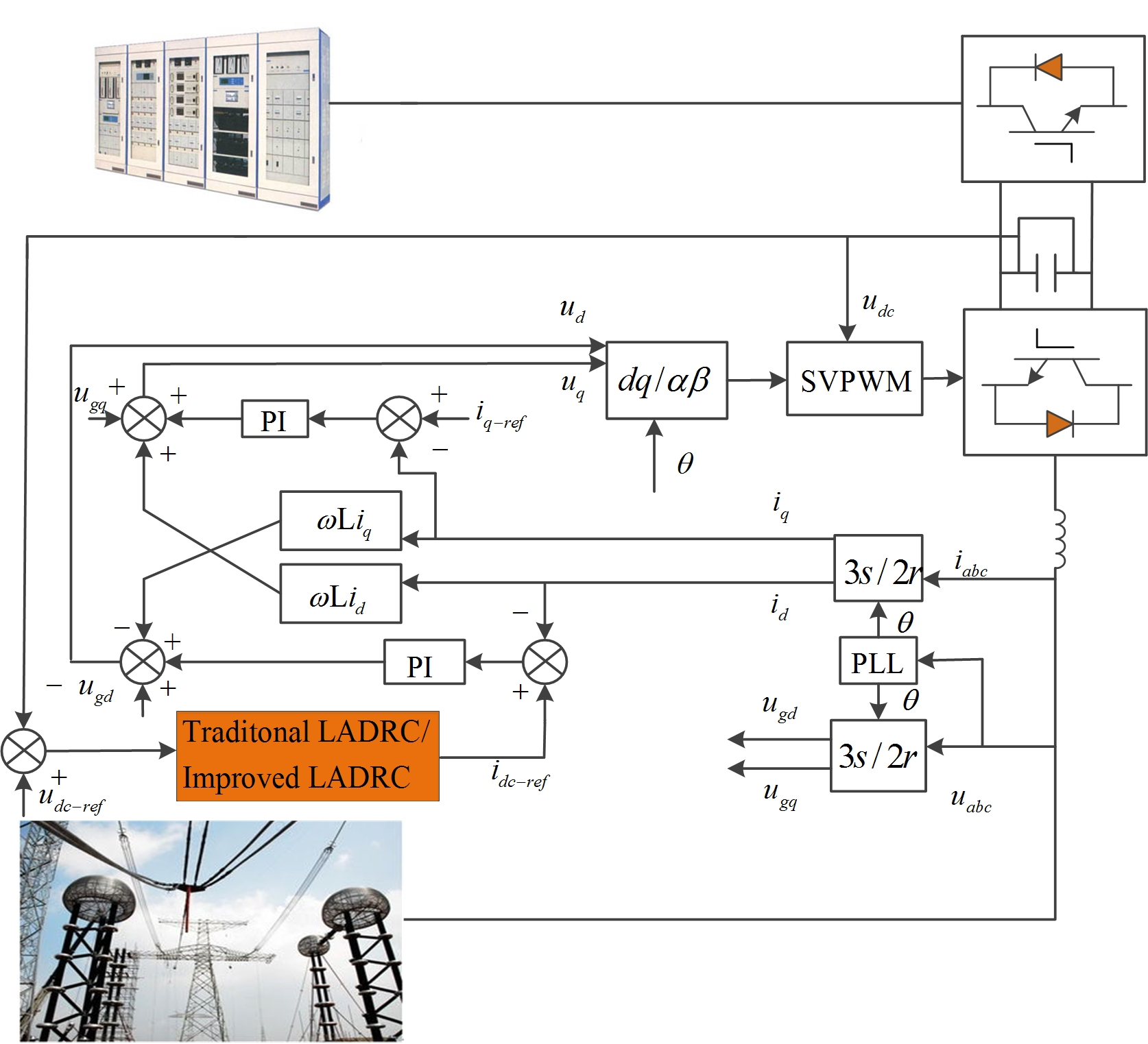
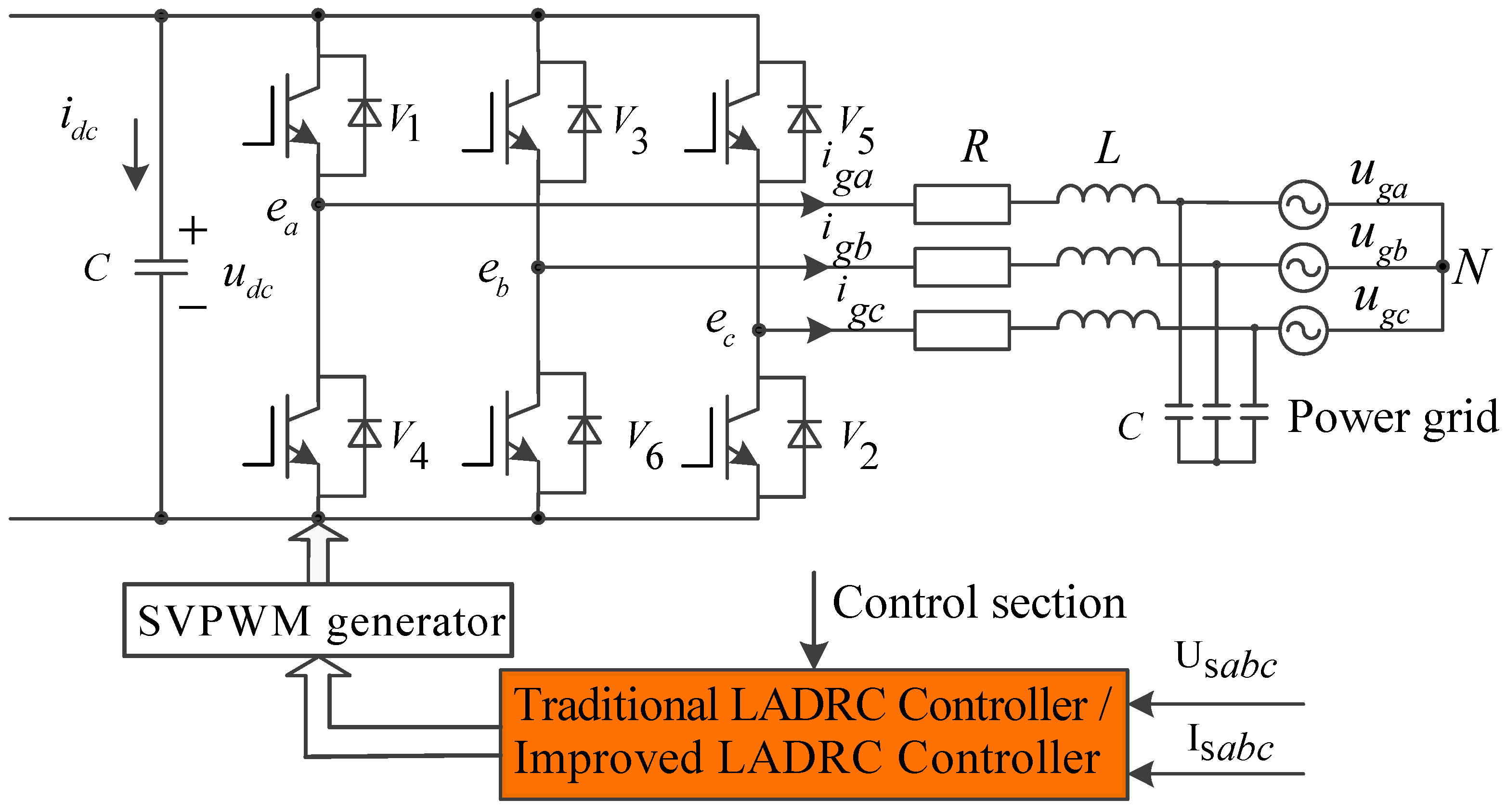
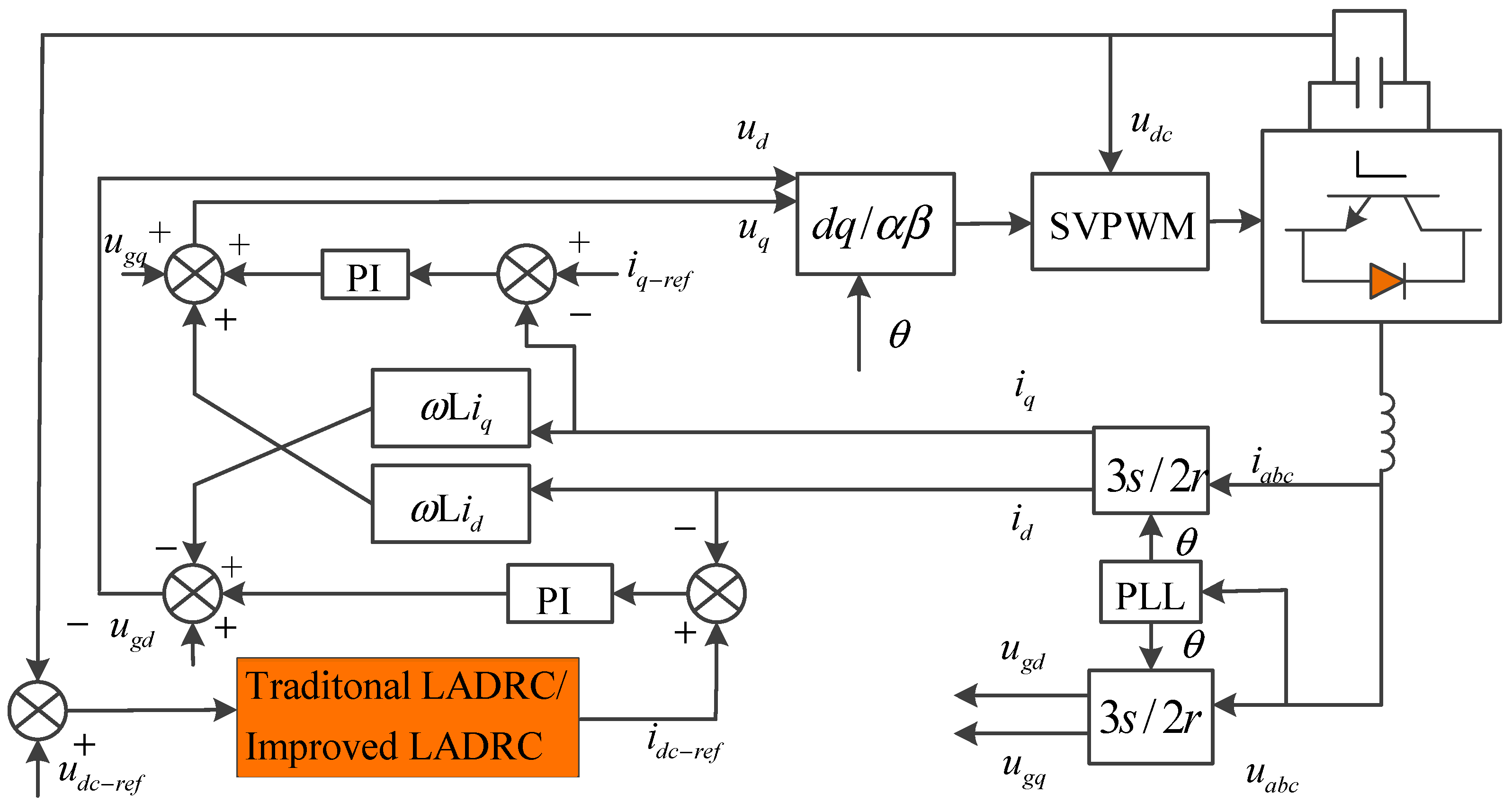
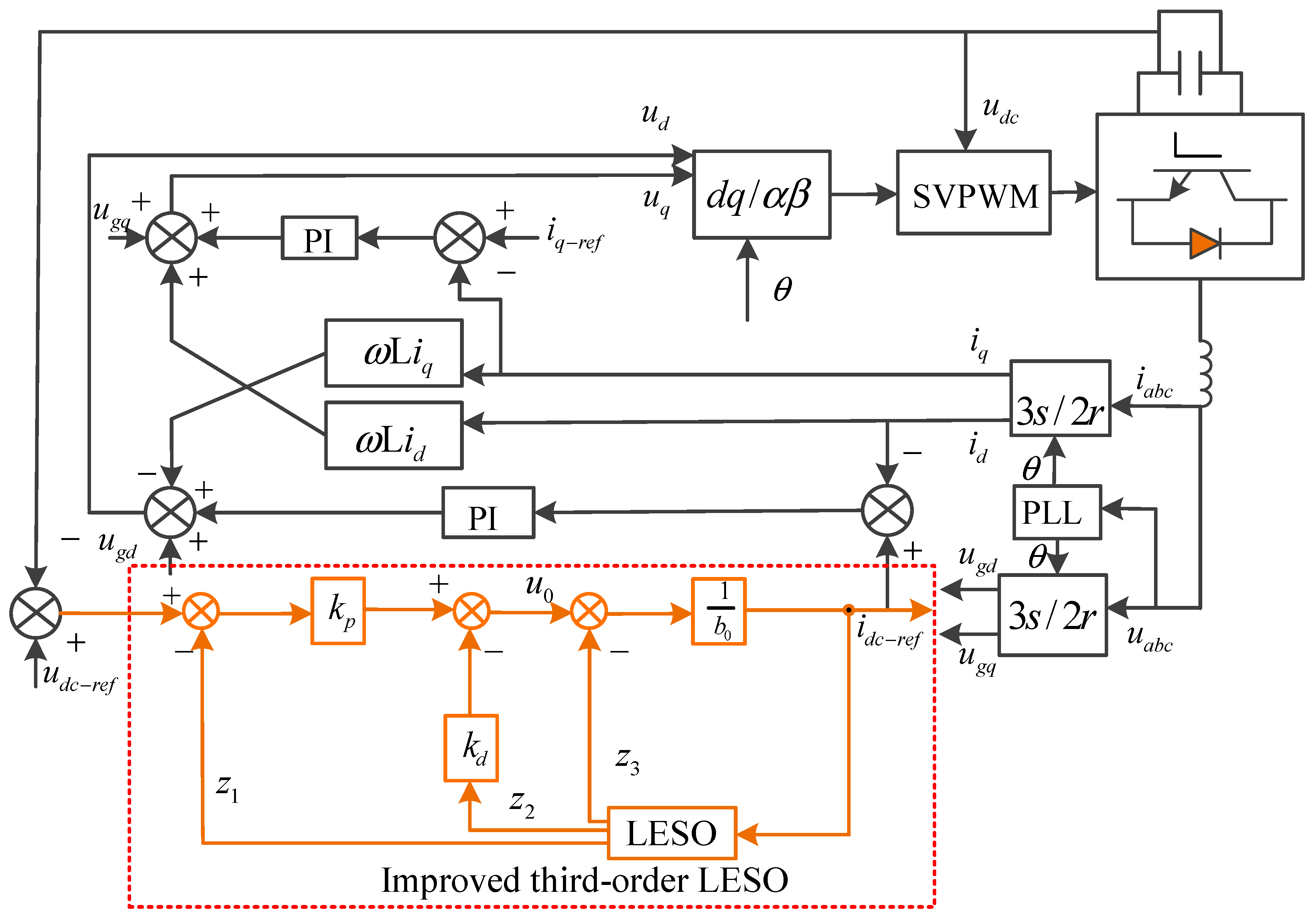
2. Mathematical Modeling of Grid-Side Inverter of Energy Storage System

The overall control structure of the grid-side inverter of the energy storage system [16] is shown in Figure 1, where u d c is representative of the voltage of the DC side bus and i d c is the current through the DC bus capacitor; R is the internal resistance of the filter inductance, L is the filter inductance and C is the filter capacitance; u g a , u g b and u g c are representative of the three-phase grid voltage; i g a , i g b and i g c are the output current of the inverter, respectively; V i ,   ( i = 1 , 2 , 3 , 4 , 5 , 6 ) are wholly controlled switching devices Insulated Gate Bipolar Transistors (IGBTs) on the six bridge arms of the inverter. e a , e b , and e c are AC output voltages of the converter; U s a b c depict three-phase voltage at the inverter side and output side, and I s a b c is the three-phase current output. The control structure of grid-connected inverter has two parts: the Space Vector Pulse Width Modulation (SVPWM) hardware layer, and the control layer, which control methods are traditional Linear Active Disturbance Rejection Control (LADRC) and improved LADRC.
The reference direction is set as the incoming current direction. According to the main circuit equivalent model, the voltage equation of grid-connected inverter is as follows [17,18]:
[ e a e b e c ] = [ u g a u g b u g c ] + L [ d i g a d t d i g b d t d i g c d t ] + R [ i g a i g b i g c ]
It can be seen from Equation (1) that the design of the control system is complicated because the three-phase current is coupled with each other and is time variable in the time domain. Therefore, the coordinate transformation method is used to transform the mathematical model of converter in three-phase static coordinate system into two-phase synchronous rotation coordinate system. The transformation matrix is as follows:
T a b c / d q 0 = 2 3 [ cos θ cos ( θ 2 π / 3 ) cos ( θ + 2 π / 3 ) sin θ sin ( θ 2 π / 3 ) sin ( θ + 2 π / 3 ) 2 / 2 2 / 2 2 / 2 ]
In Equation (2), θ = ω t + θ 0 is the phase angle of P a r k transformation, that is, the angle between the a axis in the static three-phase a b c coordinate system and the d axis in the rotating d q 0 coordinate system, where θ 0 is the initial phase angle.
After P a r k transforming Equation (1), the grid-side grid-connected inverter voltage equation in the synchronous rotating coordinate system is obtained:
[ u g d u g q ] = R [ i d i q ] + L [ d i d d t d i q d t ] + ω L [ i q i d ] + [ u d u q ]
In Equation (3), where u g d and u g q represent the components of grid voltage on the d q -axis respectively; i d and i q represent the components of the grid current on the d q -axis; u d and u q represent the components of the inverter output voltage on the d q -axis. If the phasor is three-phase symmetrical, the projection on axis d is E m , and the projection on axis q is 0, then the output voltage u g d = E m , u g q = 0 , E m of grid-side grid-connected inverter is the amplitude of phase voltage, and Equation (3) can be simplified as follows:
{ u d = ( R i d + L d i d d t ) + ω L i q + E u q = ( R i q + L d i q d t ) ω L i d
If the reference voltage and power are selected, and the system parameter adopts the unit value, the instantaneous output power of grid-connected inverter [19] can be obtained:
{ P = u d i d + u q i q Q = u q i d u d i q
If the grid voltage is stable, the decoupling control of active power and reactive power can be realized by changing the d and q axis components of grid current. In the d q 0 coordinate system, the calculated reference current is compared with the actual current output from the grid, and the deviation value of the current is obtained. After PI regulator, the command voltage is obtained, and then it is transformed from the rotating coordinate system to the static coordinate system. Finally, the on–off of the switching tube is controlled by SVPWM to control the DC-side bus voltage. The control structure of grid-side grid-connected inverter is shown in Figure 2.
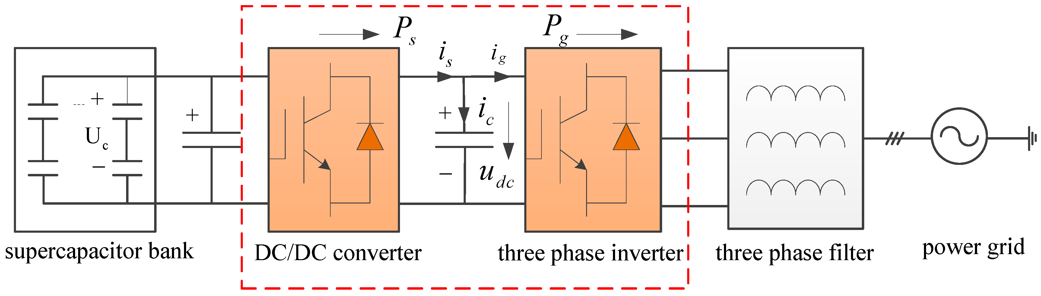
In the actual project, the grid connection of the system will be realized through a grid connection switch to realize the grid connection and off grid operation of the energy storage system [20]. When the grid voltage drops, the voltage of the grid-connected inverter also decreases. If the original input power is maintained, it will exceed the upper limit of the current regulation, which will inevitably lead to the increase of the grid-connected output current, and components will be destroyed by over-current at this time. If the control current is below the upper limit, it will lead to the imbalance of the input and output power, resulting in the sharp rise of the DC-side voltage. Therefore, the impact of grid voltage sags on the transient characteristics of grid-connected energy storage systems will be analyzed from the perspective of energy. The schematic is shown in Figure 3.
The active power P s of the super-capacitor energy storage system is input into the intermediate DC bus after passing through the DC/DC converter, ignoring the loss of the DC/DC converter, and the output power P s of the energy storage system is equal to the grid-connected input power, which can be expressed by the following equation:
P s = u d c i s
In Equation (6), where i s is the DC current output by DC/DC converter.
The current i c flowing through the DC-side capacitor is:
i c = c d u d c d t = i s i g
If the losses of the grid-connected inverter and the AC-side reactor are not considered, then the power input by the inverter from the DC-side to the grid can be expressed by Equation (8):
P g = u g d i d + u g q i q = u d c i g
In Equation (8), i d and i q represent the d and q axis components of grid-side current, i g stands for grid-side input current.
When the grid voltage remains stable, the power of both sides of the grid-connected inverter keeps balance. From Equations (6), (7) and Equation (8) will be obtained:
c u d c d u d c d t = u d c i s u d c i g = P s P g = Δ p
The power stored in the DC-side bus capacitance C is:
c u d c d u d c d t Δ T = ( P s P g ) Δ T = Δ P Δ T
From the analysis of Equation (9), it can be seen that under the normal condition of power grid, if the voltage u d c at the DC-side remains unchanged, then the value Δ P is zero.
When the grid voltage drops suddenly, the output current of grid-connected inverter is generally required to be no more than 1.1 times of the rated value. In order to limit the damage of components of grid-connected inverter due to over-current, it is necessary to keep the output current of grid-connected inverter within the upper limit of control. Its i d and i q remain unchanged, the output power P g of grid connection will inevitably decrease, while the input power P s of energy storage system will not change in a short time, which will lead to power imbalance at both ends of grid-connected inverter, and it is likely that the DC-side capacitance will be continuously increased due to the injected power. If the capacitance voltage rises too high, the DC-side capacitance will be broken down, which will eventually lead to the collapse of the whole system. Therefore, it is very important to design a controller with excellent performance to ensure the stability of DC-side bus voltage for the safety of the whole system.

3. Principle Analysis of Traditional LADRC

Traditional LADRC takes LESO as the control core, and the advantage of LESO is low model degree [13]. In addition to providing the observation values of all order state variables of the system, it can also estimate and compensate the total disturbance of the system in real time. When the estimation ability of LESO disturbance is enough, the system can be compensated into integral series type. Then, the expected performance index can be obtained through simple control rate.

3.1. Design of Traditional Third-Order LESO

Generally, the differential equation of the second-order system is taken as an example for analysis:
y ¨ = a 1 y ˙ a 0 y + w + b u
In Equation (11), where u is the input and y is output of the system, w represent external disturbance, a 0 and a 1 are the parameters of the system, b is the input control gain, and b 0 is the gain estimate. Let x 1 = y , x 2 = y ˙ , define f ( y , y ˙ , w ) = a 1 y ˙ a 0 y + w + ( b b 0 ) u as the system disturbance, and let x 3 = f ( y , y ˙ , w ) , h = f ˙ ( y , y ˙ , w ) , the equation of the system can be obtained:
[ x ˙ 1 x ˙ 2 x ˙ 3 ] = [ 0 1 0 0 0 1 0 0 0 ] [ x 1 x 2 x 3 ] + [ 0 b 0 0 ] u + [ 0 0 1 ] h
From Equation (12) we can get the following equation:
[ z ˙ 1 z ˙ 2 z ˙ 3 ] = [ β 1 1 0 β 2 0 1 β 3 0 0 ] [ z 1 z 2 z 3 ] + [ 0 b 0 0 ] u + [ β 1 β 2 β 3 ] y
In Equation (13), where β 1 , β 2 and β 3 are the coefficients of the observer, respectively.
Take the control law of the system as:
u = z 3 + u 0 b 0
The Linear State Error Feedback (LSEF) can be designed as [13]:
u 0 = k p ( v z 1 ) k d z 2
In Equation (15), where k p and k d represent the proportional and differential control gains, respectively, and the system can be stabilized by selecting the appropriate proportional differential gain coefficient.
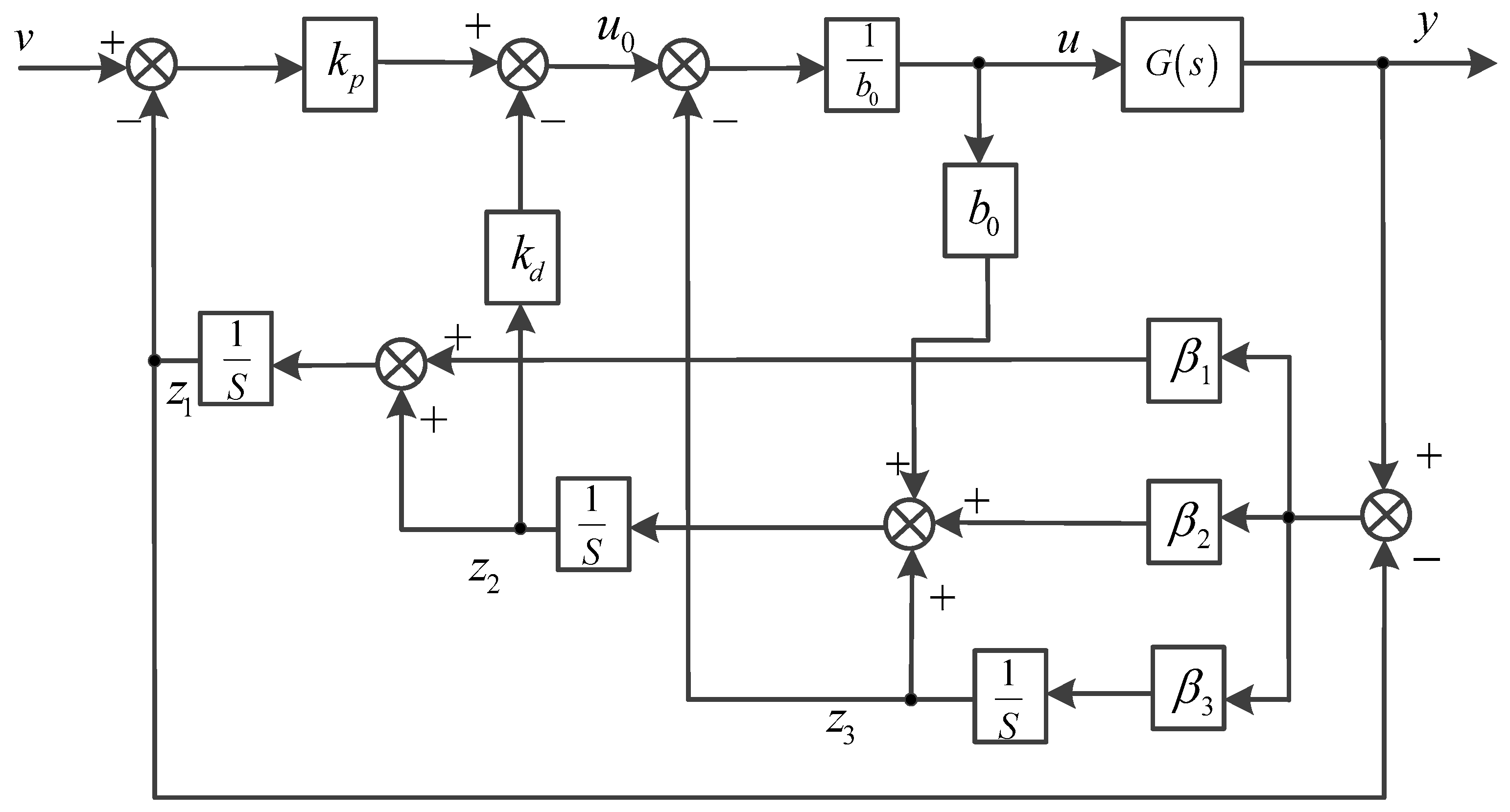
Equations (13), (14) and (15) constitute the structural block diagram of LADRC of system Equation (11), as shown in Figure 4:

3.2. Parameter Tuning of Traditional Second-Order LADRC

In traditional LADRC, the parameters of LESO and Linear State Error Feedback (LSEF) rate are mainly adjusted [13]. The parameters that need to be designed for the two are: observer gain coefficients β 1 , β 2 and β 3 of LESO, and controller parameters k p and k d of LSEF. According to the separation principle [21], parameter design can be performed for each part separately.

3.2.1. Parameter Design of Third-Order LESO

According to the pole configuration, the pole of Equation (13) is arranged on the bandwidth of the observer:
λ ( s ) = s 3 + β 1 s 2 + β 2 s + β 3 = ( s + ω 0 ) 3
Then
β 1 = 3 ω 0 ,   β 2 = 3 ω 0 2 ,   β 3 = ω 0 3
In Equation (17), ω 0 belongs to the observer bandwidth. Therefore, it is obvious from observation formula (17) that for LESO, only the parameter ω 0 
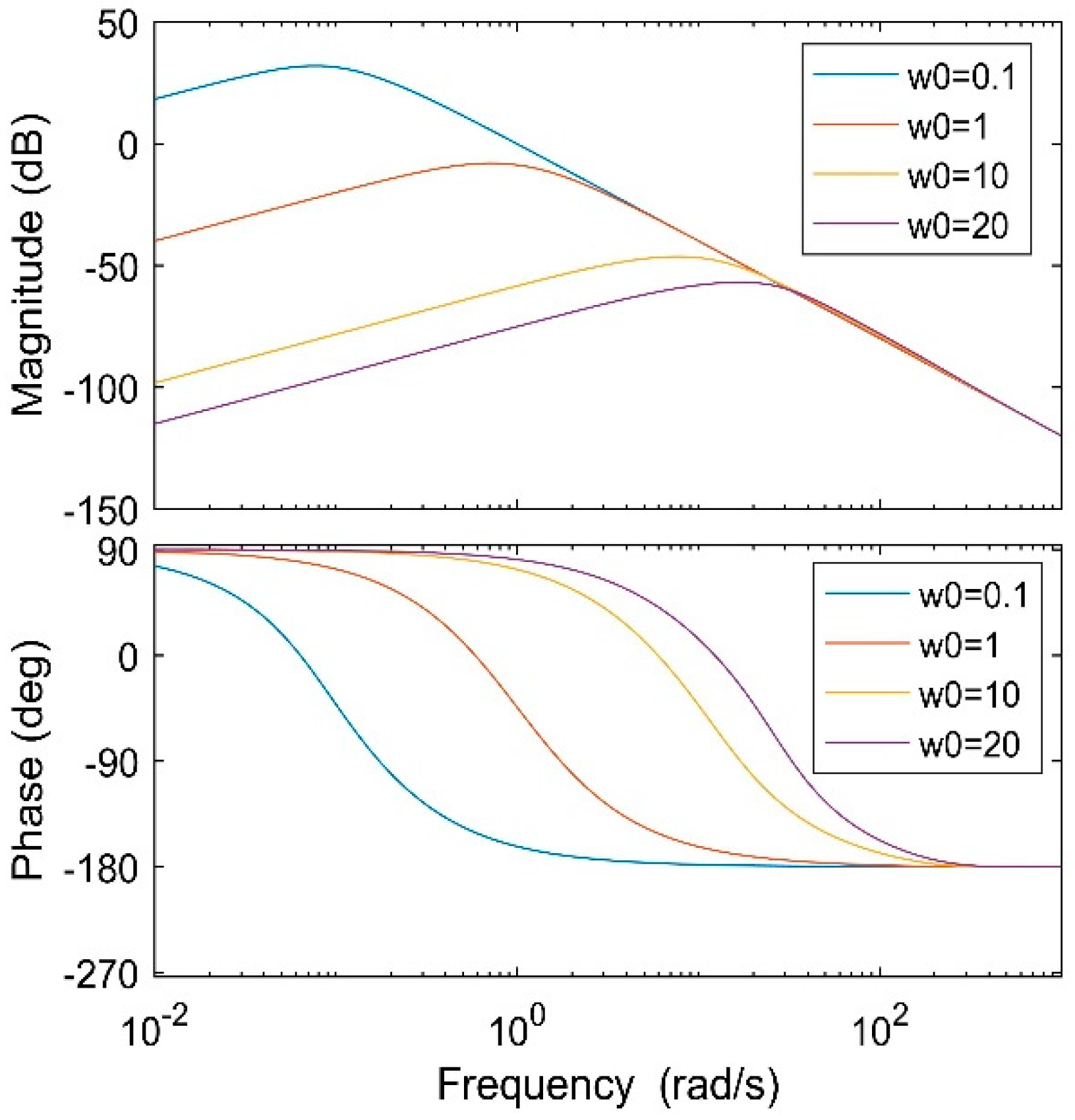
needs to be designed. The larger ω 0 , the larger the observation bandwidth of LESO, and the better the tracking effect [22]. However, during the parameter adjustment process, it will be found that too large ω 0 will also reduce the system’s immunity. Therefore, in actual engineering, the design of the observer bandwidth ω 0 should not be too large.

3.2.2. Parameter Design of LSEF

According to Reference [14], a controller with linear Proportional Differential (PD) control is adopted, and the controller corresponding to the n + 1 order LESO can take the characteristic polynomial of the closed-loop system through parameterization:
s n + k d n 1 s n 1 + + k d 1 s + k p = ( s + ω c ) n
In Equation (18), where k p , k d 1 …, k d n 1 represent the gain of the controller to be designed, respectively, ω c is the bandwidth of the controller. Through the above relationship, the proportional and differential gain of the controller can be obtained by determining the size of ω c . According to Equation (18), the gain of PD controller corresponding to third-order LESO can be obtained:
k p = ω c 2 ,   k d = 2 ω c
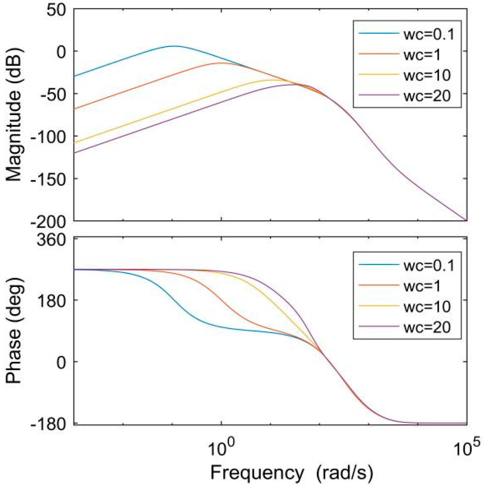
Therefore, after parameterization, the controller bandwidth ω c is the only parameter that needs to be designed in the PD controller. A larger value of ω c can make the output response of the system faster and the dynamic process time becomes shorter. However, in the process of adjusting the parameters, it will be found that too large a value of ω c will increase the load of the PD controller, which will increase the sensitivity of the system to noise, and in severe cases will cause system instability. Therefore, in the application of actual engineering, it is necessary to design the system parameters reasonably in combination with the fastness and stability of the system.
For the controller used in this paper, in the process of adjusting parameters, the general principle is to keep ω c unchanged, and then gradually increase ω 0 , until the value of ω 0 makes the effect of noise meet the system requirements. Then gradually increase ω c , reduce ω 0 when the influence of noise is unbearable, and then increase ω c to achieve the desired control effect. Finally, through the experience of adjusting the aforementioned parameters, we can determine that the LADRC parameters of the voltage outer loop are ω c = 3500 and ω 0 = 500.

3.3. Performance Analysis of Traditional Third-Order LESO

According to Equations (13) and (17), the transfer functions of Z 1 , Z 2 , and Z 3 can be obtained:
{ Z 1 = 3 ω 0 s 2 + 3 ω 0 2 s + ω 0 3 ( s + ω 0 ) 3 y + b 0 s ( s + ω 0 ) 3 u Z 2 = 3 ω 0 2 s 2 + ω 0 3 s ( s + ω 0 ) 3 y + b 0 ( s + 3 ω 0 ) s ( s + ω 0 ) 3 u Z 3 = ω 0 3 s 2 ( s + ω 0 ) 3 y b 0 ω 0 3 ( s + ω 0 ) 3 u
Make the tracking errors e 1 = z 1 y , e 2 = z 2 y ˙ will be obtained:
{ e 1 = s 3 ( s + ω 0 ) 3 y + b 0 s ( s + ω 0 ) 3 u e 2 = ( s + 3 ω 0 ) s 3 ( s + ω 0 ) 3 y + b 0 s ( s + ω 0 ) 3 u
Make e 3 = z 3 f ( y , y ˙ , w ) , according to Equation (12) will be configured as follows:
f ( y , y ˙ , w ) = x 3 = x ˙ 2 b 0 u = y ¨ b 0 u
Then
e 3 = z 3 y ¨ + b 0 u = b 0 ( 1 ω 0 3 ( s + ω 0 ) 3 ) u ( 1 ω 0 3 ( s + ω 0 ) 3 ) s 2 y
Considering the analysis typicality, y and u take the step signal y ( s ) = K / s , u ( s ) = K / s whose amplitude is K , then the steady-state error can be obtained as:
{ e 1 s = lim s e 1 = 0 s 0 e 2 s = lim s e 2 = 0 s 0 e 3 s = lim s e 3 = 0 s 0
The above equation shows that LESO has good convergence and estimation ability.
The following further analyzes the dynamic tracking process. When b 0 = 0 , the response of Z 1 in Equation (20) to step signal y ( s ) = K / s will be:
Z 1 = 3 ω 0 s 2 + 3 ω 0 2 s + ω 0 3 ( s + ω 0 ) 3 K s = K ( 1 s 1 s + ω 0 + 2 ω 0 ( s + ω 0 ) 2 ω 0 2 ( s + ω 0 ) 3 )
By inverse Laplace transformation:
Z 1 ( t ) = K K ( 1 2 ω 0 2 t 2 2 ω 0 t + 1 ) e ω 0 t
Make Z ˙ 1 ( t ) = 0 get the extreme point as:
t 1 = ( 3 3 ) / ω 0 ,   t 2 = ( 3 + 3 ) / ω 0
According to Equation (27), although ω 0 does not affect the overshoot, it will affect the tracking speed of LESO. The larger ω 0 is, the faster the system response is. Therefore, in order to improve the tracking speed, it is more likely to improve the ω 0 . However, in the actual system, the size of ω 0 is limited by the observation noise, and the increase of ω 0 will also make the observation noise amplified, which will affect the control performance of the whole controller. Therefore, it is necessary to improve the traditional LADRC so that when ω 0 increases, the effect of the observation noise on the system is relatively small.

4. Structural Design and Performance Analysis of Improved LADRC

4.1. Design Principle of Improved LESO

According to Equations (20) and (22), the third-order LESO disturbance observation transfer function can be obtained:
ϕ ( s ) = β 3 s 3 + β 1 s 2 + β 2 s + β 3
ϕ ( s ) is a third-order system. Because the theoretical analysis of the third-order system is too complex, on the other hand, because its frequency characteristics are similar to the standard second-order system in the middle and low frequency range, the third-order system can be approximately equivalent to the second-order system for analysis:
ϕ ( s ) β 3 β 1 s 2 + β 2 s + β 3 = β 3 / β 1 s 2 + β 2 / β 1 s + β 3 / β 1
ϕ ( s ) is a second-order system, it can be proved that there is a contradiction between response speed and overshoot in time domain. In frequency domain, ϕ ( s ) has the characteristics of phase lag and amplitude attenuation with the increase of frequency, which shows that the disturbance observation performance of traditional LESO is defective.
According to the comparison between Equation (29) and the standard second-order system, it can be seen that:
w n = β 3 β 1 ,   ζ = β 2 β 1 β 3
In Equation (30), where w n is the undamped natural oscillation angular frequency of the system while ζ is the damping ratio of the system.
In the standard second-order system, the time response and frequency response mainly depend on w n and ζ . From Equation (30), it can be seen that the changes of w n and ζ affect the changes of β 1 , β 2 and β 3 gains, and the changes of β 3 gain can affect w n and ζ at the same time. In short, among the three parameters, β 3 has the greatest impact on the system performance.
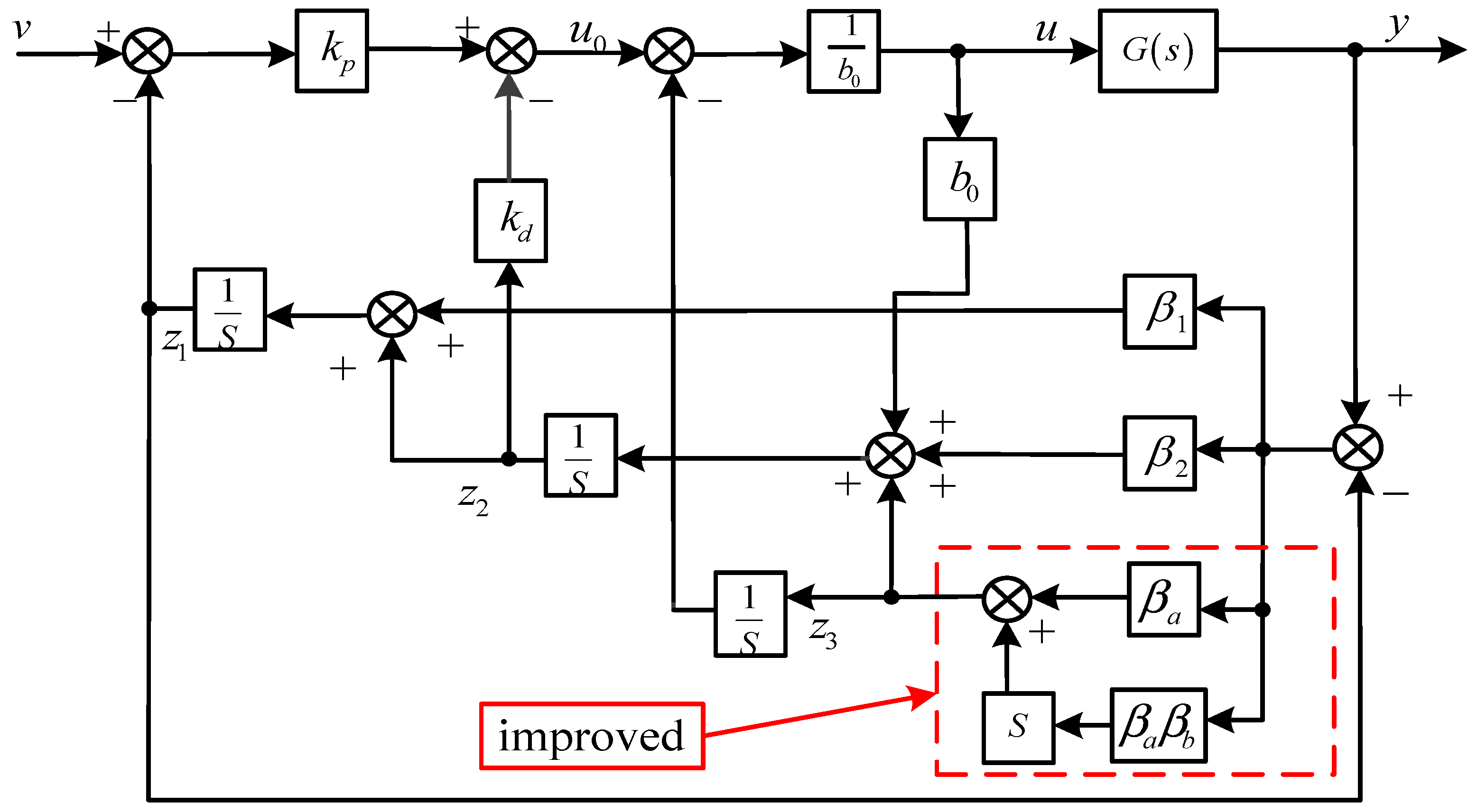
Through the above derivation and simple analysis, it can be seen that the traditional observation structure of LESO is similar to the standard second-order system, and there are some deficiencies in the structure, resulting in the increase of disturbance frequency, the observation ability of disturbance will be lower and lower. Therefore, an improved linear extended state observer is proposed by improving the observation gain coefficient β 3 of traditional LESO in this paper, which can effectively reduce the decrease of disturbance observation amplitude and phase lag, and then improve the disturbance rejection ability of LADRC. The improved equation is as follows:
β 3 ( s ) = β a ( 1 + β b s )
In Equation (31), where β a and β b are proportional differential coefficients, respectively, and the improved β 3 includes the proportional differential link. At this time, the transfer function of disturbance observation can be expressed as:
ϕ ( s ) = β a ( 1 + β b s ) s 3 + β 1 s 2 + ( β 2 + β a β b ) s + β a
Compared with Equation (32) and Equation (28), the most obvious change is the addition of a zero point. In the control theory, it can be understood as follows: in the time domain, the function of zero point is to reduce the peak time, speed up the response speed of the system, and the closer the zero point is to the virtual axis, the more obvious the effect is; in the frequency domain, a leading network is connected in series, which reduces the slope of amplitude decline and the degree of phase lag, and improves the stability of the system.
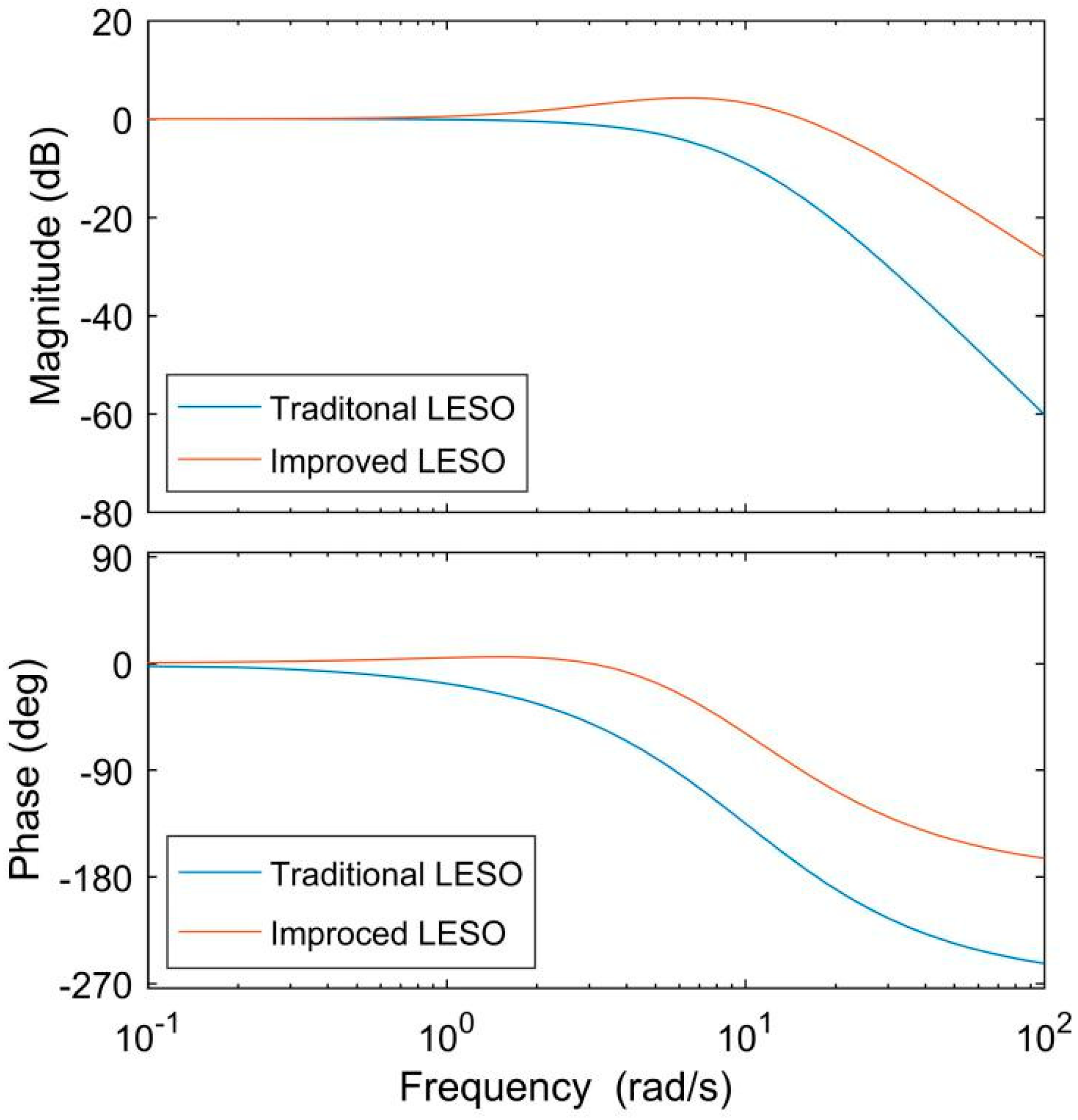
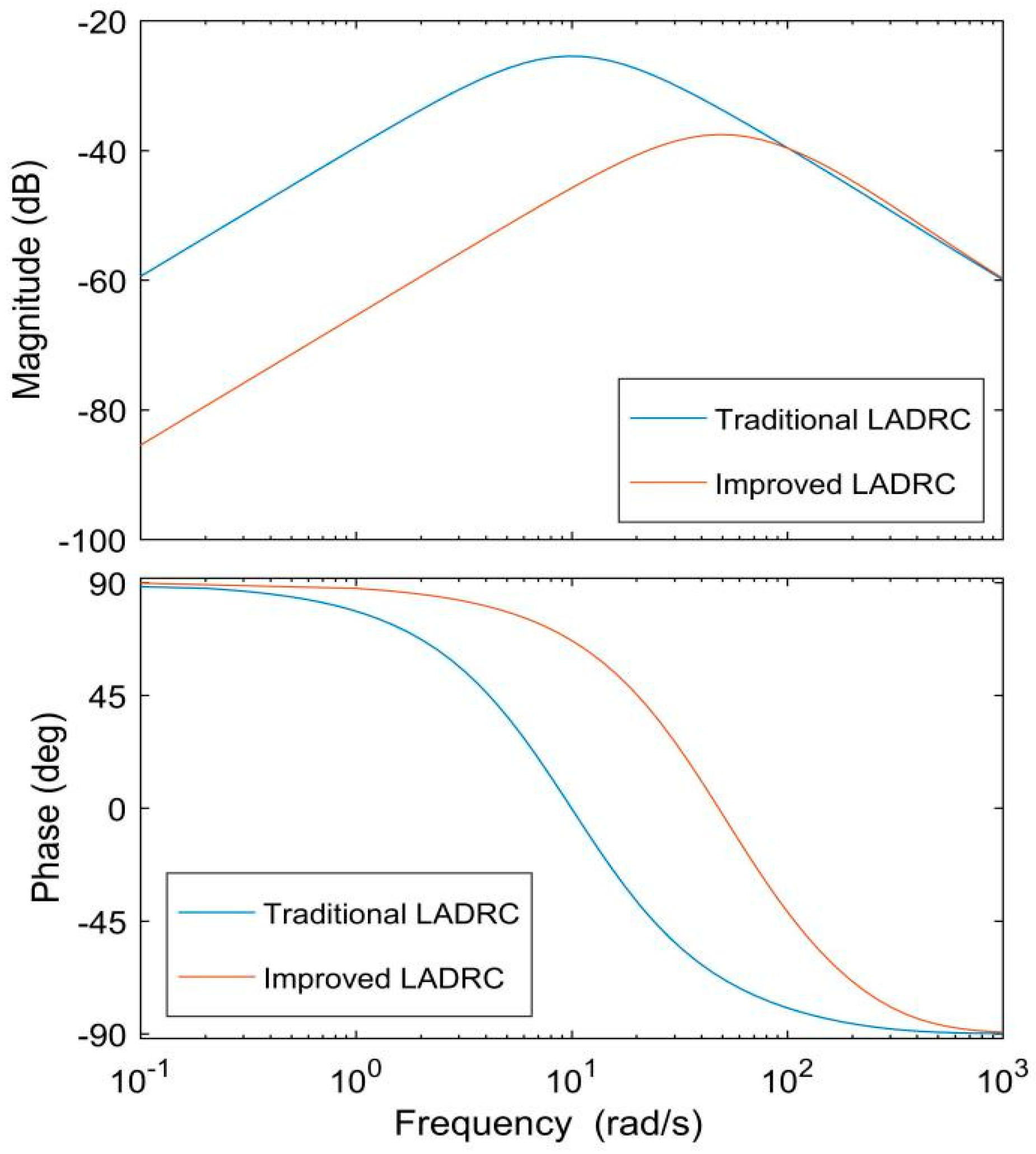
Figure 5 shows the amplitude frequency and phase frequency characteristic curve of the disturbance transfer function of traditional LESO and improved LESO. The bandwidth and phase characteristics in the middle and low frequency range do not change significantly with the increase of frequency, and the index attenuation capacity at the high frequency is obviously slowed down. Compared with traditional LESO, the observation ability of improved LESO to disturbance is improved, the slope of amplitude decrease and the degree of phase lag are reduced, and the stability of the system is improved. The feasibility and effectiveness of improved LESO are proved.

4.2. Structural Design of Improved LADRC

According to Equation (20) and Equation (31), the transfer functions of improved Z 1 , Z 2 and Z 3 can be obtained as follows:
{ Z 1 = 3 ω 0 s 2 + 3 ω 0 2 s + ω 0 3 ( s + ω 0 ) 3 y + b 0 s ( s + ω 0 ) 3 u Z 2 = 3 ω 0 2 s 2 + ω 0 3 s ( s + ω 0 ) 3 y + b 0 ( s + 3 ω 0 ) s ( s + ω 0 ) 3 u Z 3 = ω 0 3 s 2 + ω 0 3 β b s 3 ( s + ω 0 ) 3 y b 0 ω 0 3 + b 0 ω 0 3 β b s ( s + ω 0 ) 3 u
In conclusion, according to Equation (14) and Equation (32), the structure of improved LADRC control system is as follows Figure 6:
Combining Equations (14), (15), and (19) can be expressed as the following equation:
u = 1 b 0 ( ω c 2 ( v z 1 ) 2 ω c z 2 z 3 )
Substituting Equation (33) into Equation (34) can be obtained as follows:
u = 1 b 0 G 1 ( s ) [ ω c 2 v H ( s ) y ]
In Equation (35):
G 1 ( s ) = ( s + ω 0 ) 3 s 3 + 3 ω 0 s 2 + 3 ω 0 2 s + ω c 2 s + 2 ω c s 2 + 6 ω 0 ω c s ω 0 3 β b s
H ( s ) = ω 0 3 β b s 3 + ( 3 ω 0 ω c 2 + ω 0 3 ) s 2 + ( 3 ω 0 2 ω c 2 + 2 ω c ω 0 3 ) s + ω c ω 0 3 + 6 ω c ω 0 2 ( s + ω 0 ) 3
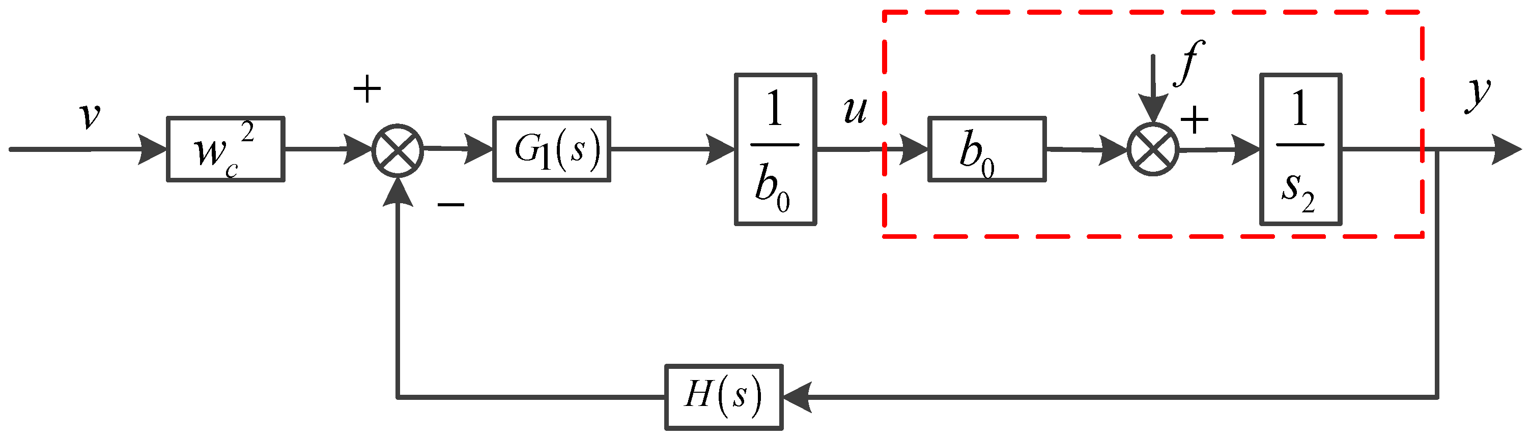
According to Equation (12), the controlled object can be recorded as:
y = 1 s 2 ( f + b 0 u )
Simultaneous Equation (35) and Equation (36) can simplify the improved LADRC control system to be:
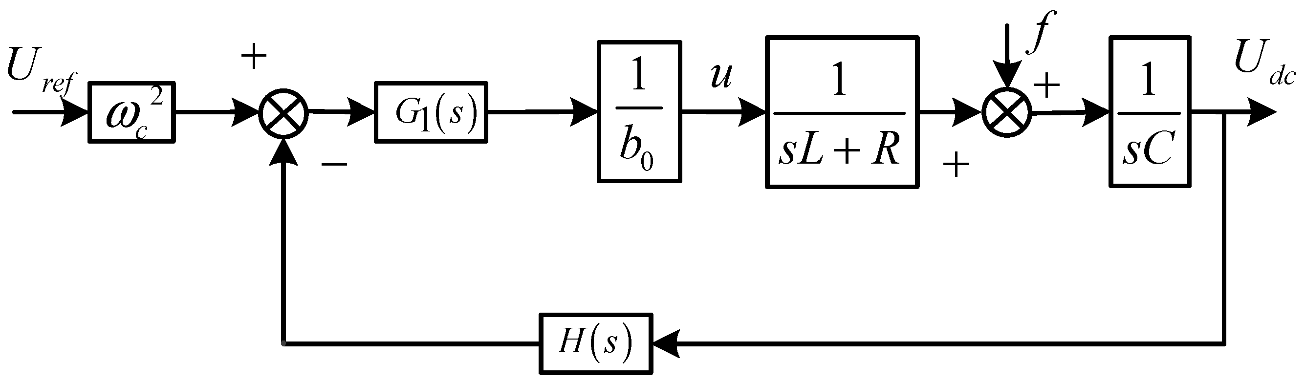
According to Figure 7, the closed-loop transfer function of the system can be obtained by using the superposition theorem as follows:
y = G 1 ( s ) s 2 + G 1 ( s ) H ( s ) ω c 2 v + 1 s 2 + G 1 ( s ) H ( s ) f
It can be known from Equation (37) that the output of the system is composed of a tracking term and a disturbance term. When the disturbance term is ignored, the system can achieve fast and no overshoot tracking of the reference input by adjusting the controller bandwidth ω c and the observer bandwidth ω 0 .

5. Performance Analysis of Improved LADRC in Energy Storage Grid-Connected System

5.1. Structure Design of Improved LADRC in Energy Storage Grid-Connected System

According to the above analysis, an improved second-order LADRC voltage external loop controller based on the proportional differential is established. Through the above modeling of grid-side inverter, we can write the mathematical model expression of DC-side of grid-side inverter based on switch function in the d q coordinate system of two-phase synchronous rotation, as shown in Equation (38):
d u d c d t = i d c 3 2 C k = d , q S g k i g k
In Equation (38), S g k is the component of the switch function on the d, q axis.
From the simplification of Equation (38) can be obtained as follows:
d 2 u d c d t 2 = 3 2 L C k = d , q S g k ( u g k + i g k R e g k ) ω 2 C ( S g d i g q S g q i g d )
It can be seen from Equation (39) that the mathematical model of the energy storage grid-connected inverter is a second-order system, so the improved second-order LADRC based on the proportional differential can be used in the control of the energy storage inverter. Now, Equation (39) is transformed into state space form can be expressed as the following equation:
{ [ x ˙ 1 x ˙ 2 x ˙ 3 ] = [ 0 1 0 0 0 1 0 0 0 ] [ x 1 x 2 x 3 ] + [ 0 0 b 0 0 0 1 ] [ u h ] y = x 1
In Equation (39), b 0 = 3 / ( 2 L C ) , x 1 is bus voltage and x 2 is its differential, x 3 is the expanded state variable in LESO, the physical meaning is the total disturbance of the system, that is, f , h is the differential of f , and the model of the total disturbance is as follows:
f = 3 2 L C k = d , q S g k ( i g k R e g k ) ω 2 C ( S g d i g q S g q i g d ) + 3 2 L C S g q u g q
The LSEF combined with the actual system can be designed as:
{ u 0 = ω c 2 ( u d c - r e f z 1 ) 2 w c z 2 u = ( z 3 + u 0 ) / b 0 = i d c - r e f
In Equation (42), u d c - r e f is the voltage value given by the DC bus, and i d - r e f is the reference value given by the inner ring d-axis. Therefore, the improved second-order LADRC outer loop control block diagram based on the actual energy storage grid-connected inverter can be designed (see Figure 8).

5.2. Analysis of Interference Immunity Tracking of Improved LADRC in Energy Storage System

From Equation (37), it can be seen that the effect of the disturbance term is related to the bandwidth ω c of the controller and the bandwidth ω 0 of the observer.
Select ω 0 = 100, ω c = 0.1, 1, 10, 20 to get the frequency characteristic curve as shown in Figure 9; Take ω c = 100, ω 0 = 0.1, 1, 10, 20 to get the frequency characteristic curve as shown in Figure 10.
It can be known from the above two figures that the increase can make the disturbance gain decrease and the system’s anti-interference ability enhanced.
Generally, in the energy storage grid-connected system, for the grid-connected inverter, the disturbance mainly comes from the grid-side (load side) current, based on the grid current feed-forward control strategy can effectively suppress the impact of disturbance on the grid-connected voltage control [23]. In the following, we mainly analyze the influence of controller bandwidth ω c and observer bandwidth ω 0 of improved LADRC on the tracking characteristics and anti-grid voltage disturbance characteristics of the actual grid-connected energy storage system.
The control diagram of the actual energy storage grid-connected system can be obtained from Figure 8:
According to Figure 11, the voltage transfer function of DC bus output from the controlled system can be obtained:
U d c = G 1 ( s ) ω c 2 b 0 [ L C s 2 + R C s ] + G 1 ( s ) H ( s ) U r e f + b 0 ( L s + R ) b 0 [ L C s 2 + R C s ] + G 1 ( s ) H ( s ) f = C 1 ( s ) ω c 2 U r e f + C 2 ( s ) f
In Equation (43), where U d c , U r e f and f represent the DC bus voltage of the energy storage grid-connected inverter system, respectively, the reference value of the system output DC bus voltage and the grid voltage disturbance suffered by the system. C 1 ( s ) represents the transfer function from the reference value U r e f of the output DC bus voltage of the energy storage grid-connected inverter system to the actual output voltage value U d c of the system, that is, to realize the fast tracking performance (trace-ability) of the grid-connected inverter to the output voltage of the system; C 2 ( s ) represents the transfer function from the grid voltage disturbance f to the actual output voltage U d c of the system, that is, to achieve the grid-connected inverter to maintain the stability (disturbance rejection) of the DC bus voltage of the system.
It can be seen from the Figure 12 that compared with the traditional LADRC, the amplitude change of the improved LADRC control under the disturbance of the actual energy storage grid-connected system is significantly lower than that of the traditional LADRC, and the anti-interference ability is stronger. Therefore, in the energy storage grid-connected system, the improved active disturbance rejection control technology based on proportional differentiation designed in this paper has more advantages in practical systems, and also validates the effectiveness of the controller designed in this paper.

5.3. Stability Analysis of Improved LADRC in Energy Storage Systems

The influence of external disturbance and model parameter uncertainty is not considered temporarily, namely f ( t , y , y ˙ , w ) = ( b b 0 ) u ( t ) , Laplace transform is F ( s ) = ( b b 0 ) U ( s ) .
Simultaneous Equation (36) can be obtained:
y = 1 s 2 [ ( b b 0 ) U ( s ) + b 0 U ( s ) ]
According to Equation (44), the closed-loop transfer function of the system will be:
y = ( s + ω 0 3 ) ω c 2 a 5 s 5 + a 4 s 4 + a 3 s 3 + a 2 s 2 + a 1 s 1 + a 0
In Equation (45):
a 5 = b 0 L C ;   a 4 = b 0 R C + 3 ω 0 b 0 L C + 2 ω c b 0 L C a 3 = 3 ω 0 2 b 0 L C + ω c 2 b 0 L C + 6 ω 0 ω c b 0 L C + 3 ω 0 b 0 R C + 2 ω c b 0 R C + ω 0 3 β b b 0 L C ω 0 3 β b a 2 = 3 ω 0 2 b 0 R C + ω c 2 b 0 R C + 6 ω 0 ω c b 0 R C + 3 ω c 2 ω 0 b 0 R C ω 0 3 β b a 1 = 3 ω 0 2 ω c 2 + 2 ω 0 3 ω c ;   a 0 = ω 0 3 ω c 2 + 6 ω 0 2 ω c
Since the controller bandwidth ω c and observer bandwidth ω 0 are both positive, it can be seen from the parameters in Table A1 and Table A2 that a i > 0   ( i = 0 , 1 , 2 , 3 , 4 , 5 ) .
According to Liénard–Chipart stability criterion, the necessary and sufficient condition for the stability of the grid-connected inverter system is that its odd-order Hurwitz determinant is positive, namely Δ 3 > 0 , Δ 5 > 0 . According to the coefficients of Equation (45) and the parameters in Table A1 and Table A2 can be expressed as the following equation:
Δ 5 = | a 1 a 0 0 0 0 a 3 a 2 a 1 a 0 0 a 5 a 4 a 3 a 2 a 1 0 0 a 5 a 4 a 3 0 0 0 0 a 5 | > 0 ,   Δ 3 = | a 1 a 0 0 a 3 a 2 a 1 a 5 a 4 a 3 | > 0
Therefore, the energy storage grid-connected inverter system remains stable.

6. Simulation Analysis

In order to verify the effectiveness of the control strategy designed in this paper, the simulation model of grid connection of 0.3 MW super-capacitor energy storage system was established in MATLAB/Simulink. The simulation content was divided into two parts, one being the comparative analysis of the control effect of improved LADRC and traditional LADRC in the grid-connected system under steady state, the other being the comparative analysis of the control effect of the grid-side of the system under low-voltage ride-through. The main parameters of the grid-side of the super-capacitor energy storage system are shown in Table A1, and the parameters of the controller are shown in Table A2.

6.1. Comparative Analysis of Simulation in Steady State

The energy storage system operated in a stable state (without internal and external interference), and the system simulation time was 2 s. Other conditions were the same, comparing the DC-side bus voltage waveform under the two control modes of improved LADRC and traditional LADRC. At this time, the grid voltage waveform was normal and unaffected, as shown in Figure 13a. The voltage waveform of the DC-side bus under the two control modes is shown in Figure 13b.
From Figure 13b, it can be seen that the DC bus voltage fluctuation range under traditional LADRC control is significantly higher than that under improved LADRC control when the system is in stable state. Therefore, through the simulation comparison under the stable condition, the control effectiveness of improved LADRC is effectively proved.
It can be seen from Figure 14 that in improved LADRC control mode, the harmonic distortion rate of grid-connected current is significantly reduced, and the harmonic content of grid-connected current is reduced from 3.33% to 1.62%. It shows that improved LADRC has a significant role in restraining the harmonic distortion rate of grid current and improving the power quality of grid connection, and also shows the effectiveness of improved LADRC in system control.

6.2. Comparative Analysis of Simulation Under Disturbance

In fact, most of the systems work under disturbance. In order to further verify the effectiveness of the improved LADRC control in order to meet the actual needs of the system under the disturbance condition, aiming at the two different control modes of the improved LADRC and the traditional LADRC, this paper designs the grid-side low-voltage ride-through fault of the super-capacitor energy storage system, and carries out the simulation analysis of the symmetrical and asymmetric grid-side faults according to the magnitude of the low-voltage ride-through. The simulated fault conditions are as follows:
  • the voltage at the grid-side drops 30% symmetrically, falls at 0.3 s and recovers at 0.7 s;
  • the voltage at the grid-side drops by 30% asymmetrically, falls at 0.3 s and recovers at 0.7 s;
  • the voltage at the grid-side drops 60% symmetrically, falls at 0.3 s and recovers at 0.7 s;
  • the voltage at the grid-side drops by 60% asymmetrically, falls at 0.3 s and recovers at 0.7 s.
Scenario 1
Set the grid-side voltage to drop 30% symmetrically due to the low-voltage ride-through fault, when t = 0.3 s, the fault starts, when t = 0.7 s, the fault ends, and the system simulation time is 2 s, as shown in Figure 15a.
Under the same other conditions, compare the dynamic response waveform of DC-side bus voltage under 30% symmetrical voltage drop of grid-side under the two control modes, as shown in Figure 15b. Voltage fluctuation range and voltage stability are selected as important reference indices of control performance.
It can be seen from Figure 15b that the fluctuation range of the DC bus voltage controlled by traditional LADRC is 0.996p.u.–1.022p.u. during the low-voltage ride-through of 0.3p.u., while the fluctuation range of the bus voltage controlled by improved LADRC is 0.996p.u.–1.008p.u., and it can quickly reach the stable state of 1.0p.u. By comparison, improved LADRC control can promote the stability of DC bus voltage under disturbance, which shows that improved LADRC has better anti-interference performance.
Scenario 2
The model is set so that the voltage at the grid connection side drops by 30% due to the low-voltage ride-through fault asymmetry. The fault starts at t = 0.3 s, and ends at t = 0.7 s. The system simulation time is 2 s, as shown in Figure 16a.
From Figure 16b, it can be seen that the fluctuation range of traditional LADRC controlled DC bus voltage is 0.994p.u.–1.013p.u. during the low-voltage ride-through of 0.3p.u., while the fluctuation range of improved LADRC controlled bus voltage is 0.996p.u.–1.008p.u., and it can quickly reach the stable state of 1.0p.u. Compared with symmetrical faults with the same degree of sag, the fluctuation range of DC-side bus voltage is significantly reduced, but the fluctuation duration is relatively long during the fault period, which is not easy to stabilize the system. Therefore, no matter what kind of fault, improved LADRC control can promote the stability of DC bus voltage better under the disturbance condition, which shows that improved LADRC has better anti-interference performance.
Scenario 3
Set the grid-side voltage to drop 60% symmetrically due to the low-voltage ride-through fault, when t = 0.3 s, the fault starts, when t = 0.7 s, the fault ends, and the system simulation time is 2 s, as shown in Figure 17a.
From Figure 17b, it can be seen that the fluctuation range of traditional LADRC controlled DC bus voltage is 0.931p.u.–1.061p.u. during the low-voltage ride-through of 0.6p.u., while improved LADRC controlled bus voltage fluctuation range is 0.970p.u.–1.061p.u., and it can quickly reach stable state of 1.0p.u. By comparison, improved LADRC control can promote the stability of DC bus voltage under disturbance, which shows that improved LADRC has better anti-interference performance. Compared with the symmetrical voltage drop of 0.3p.u. at grid-side under Scenario 1, the fluctuation range of bus voltage at DC-side is significantly larger. Therefore, the symmetrical voltage drop at grid-side affects the fluctuation range of bus voltage at DC-side. The larger the voltage drop, the larger the fluctuation range of bus voltage at DC-side; the smaller the voltage drop, the smaller the fluctuation range of bus voltage at DC-side. Therefore, the improvement of voltage outer loop controller to ensure the stability of DC bus voltage is very important for the stable operation of the whole system.
Scenario 4
Set the voltage at the grid connection side to drop 60% due to the low-voltage ride-through fault asymmetry. The fault starts at t = 0.3 s, and ends at t = 0.7 s. The system simulation time is 2 s, as shown in Figure 18a.
It can be seen from Figure 18b that the fluctuation range of the DC bus voltage controlled by traditional LADRC is 0.990p.u.–1.029p.u. during the low-voltage ride-through of 0.6p.u., while the fluctuation range of the bus voltage controlled by improved LADRC is 0.990p.u.–1.020p.u., and it can quickly reach the stable state of 1.0p.u. In contrast, improved LADRC control can promote the stability of DC bus voltage under disturbance, which shows that improved LADRC has better anti-interference performance. It also shows that improved LADRC has good applicability under asymmetric fault.

7. Conclusions

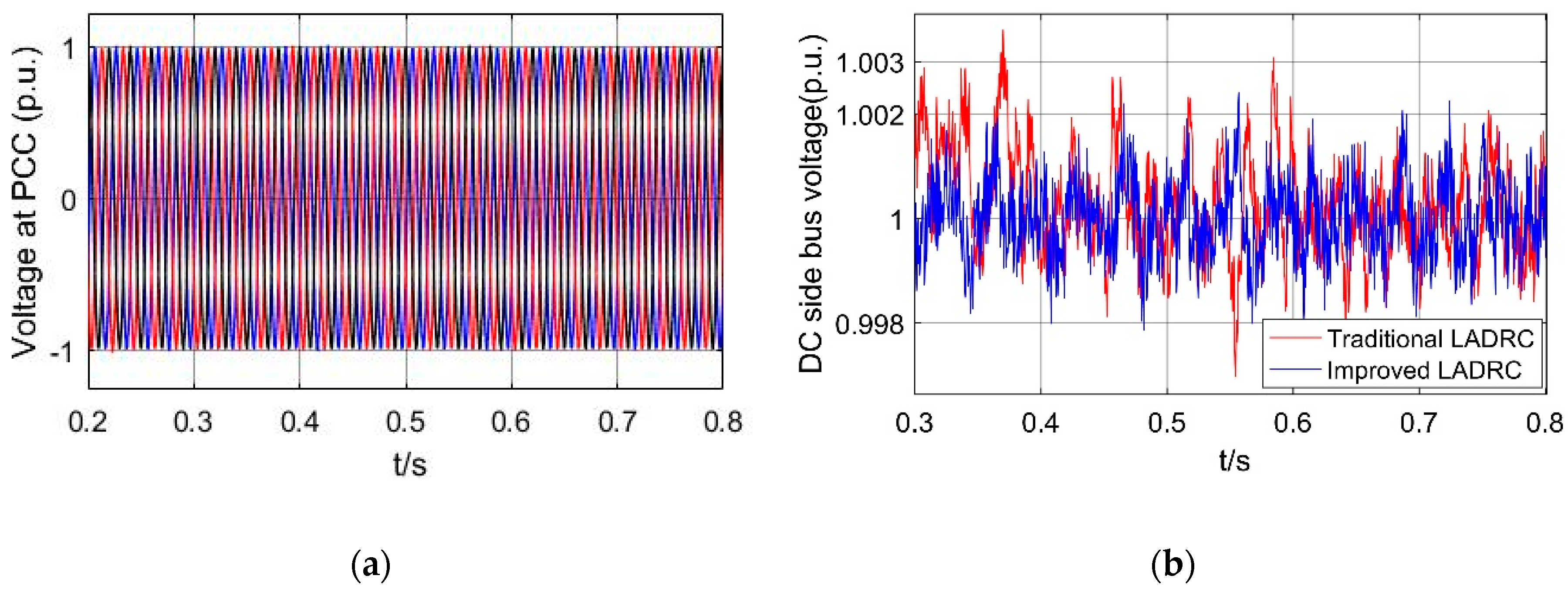
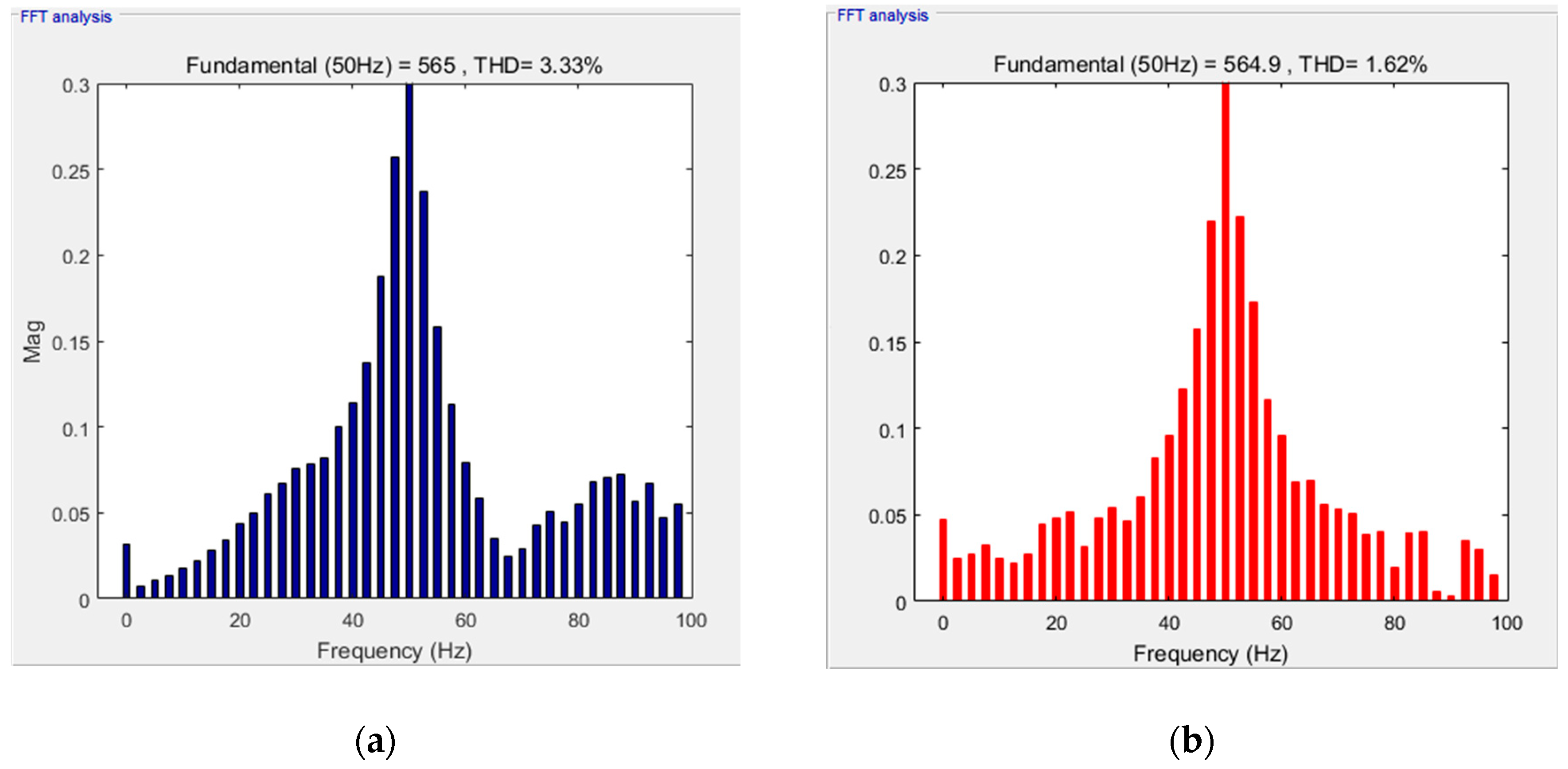
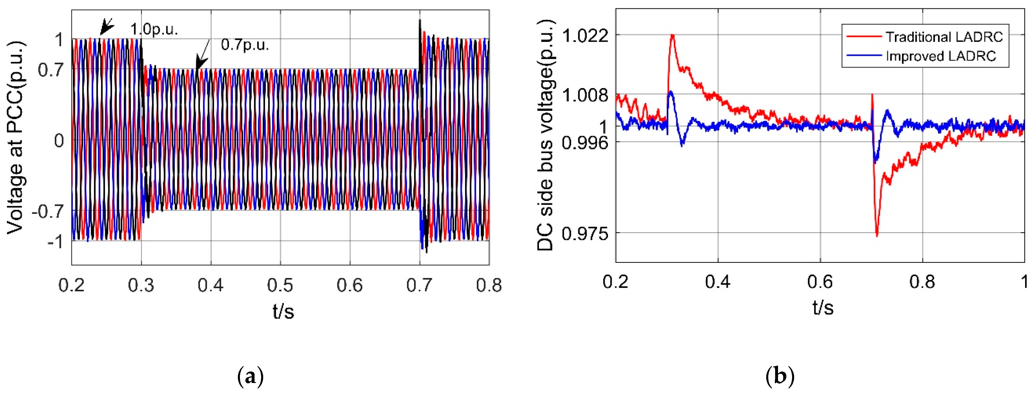
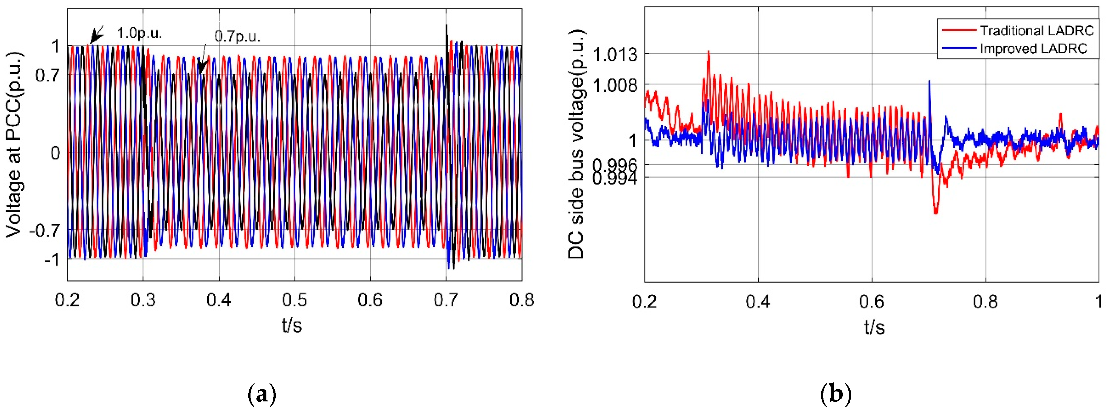
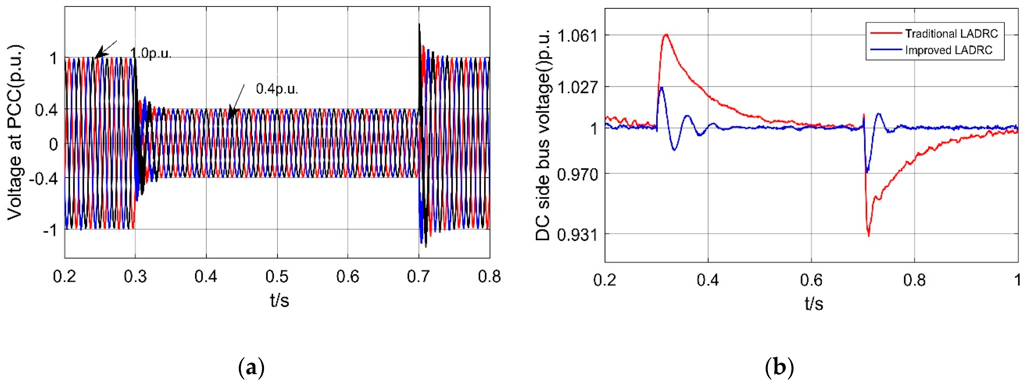
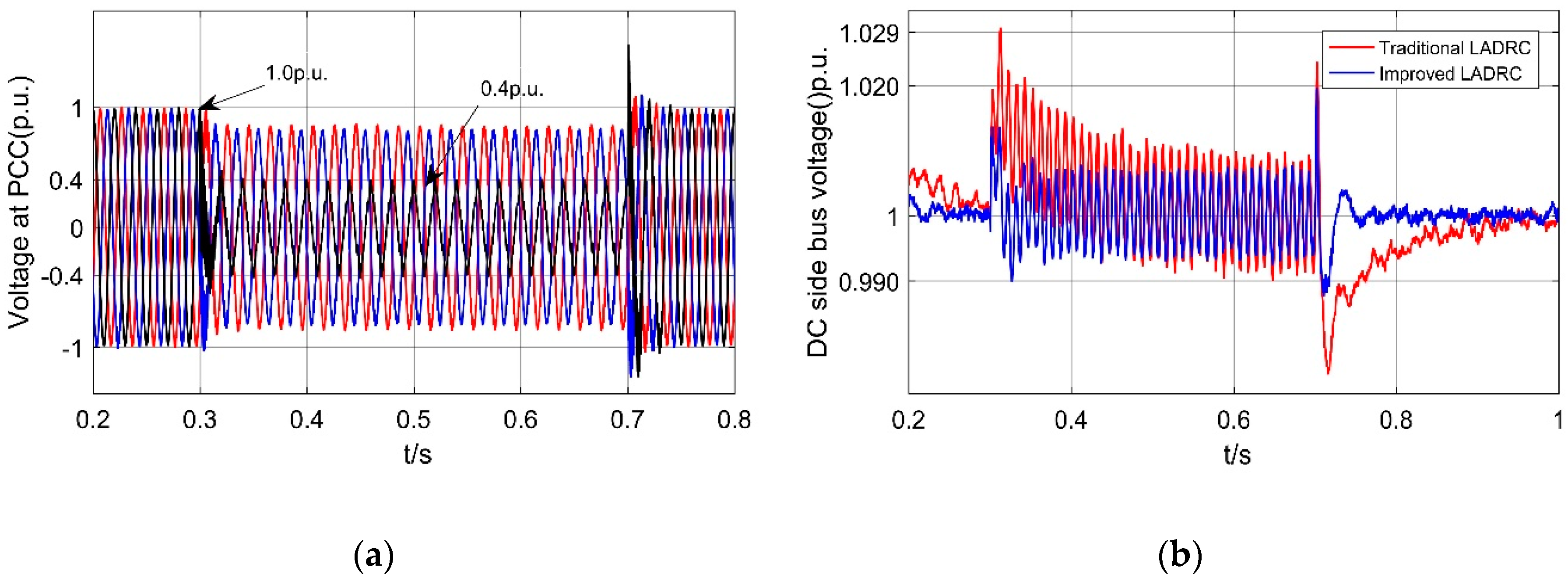
The DC-side bus voltage control of grid-connected inverter with energy storage is an important problem in the realization of stable grid-connected energy storage system. The quality of control performance directly determines the quality of grid-connected energy storage and the stability of DC-side bus voltage. In this paper, the energy storage grid-connected inverter is taken as the control object, and the DC-side bus voltage is taken as the research purpose. Aiming at the influence of low-voltage ride-through on the DC-side bus voltage, a method of improving the LADRC DC-side bus voltage based on proportional differential is proposed. The innovation of this paper is that on the basis of traditional LESO structure, the observation gain coefficient of total disturbance is improved to a proportional differential link. With the increase of frequency, the decrease of disturbance observation amplitude and phase lag are reduced effectively, the observation band width of LESO is increased, the effect of fast tracking compensation for total disturbance is achieved, at the same time, the disturbance rejection ability of the controller is improved. In this paper, the simulation analysis of symmetrical and asymmetric faults is carried out by setting 30% and 60% low-voltage ride-through at the grid-side, it is proved that the controller designed in this paper has better control performance of stabilizing DC-side bus voltage than the traditional controller.
In this paper, by improving the traditional LADRC, the control performance of the controller is obviously improved, but at the same time, the noise is amplified in the high frequency band, so that the system cannot be controlled. Therefore, the next research goal of this paper is to correct the improved LADRC link, so that the LESO is not affected by noise even in the high frequency range, so as to achieve better control effect of the controller. At the same time, we clearly realize that the biggest deficiency of this paper is the lack of physical experiments, which makes the theoretical results unable to be further verified. Therefore, in the next research, on the basis of the inadequate design of the controller in this paper, we should improve the theoretical results and carry out physical experiments, so that the theoretical results are more practical.

Author Contributions

Y.M. conceived the main idea for the proposed improved LADRC and performed overall analysis; L.Y. and X.Z. wrote this paper; X.Y., Y.Z. and B.Z. contributed to analyzing the experimental results. All authors have read and agreed to the published version of the manuscript.

Funding

This work was funded by National Natural Science foundation of China (NO. 51877152) and Natural Science Foundation of Tianjin of China (NO. 18JCZDJC97300).

Acknowledgments

The authors are grateful to the support by the National Natural Science foundation of China (NO. 51877152), Natural Science Foundation of Tianjin of China (NO. 18JCZDJC97300) and Tianjin University of Technology for their support.

Conflicts of Interest

The authors declare no conflicts of interest.

Abbreviations

LADRCLinear Active Disturbance Rejection Control
LESOLinear Extended State Observer
ADRCActive Disturbance Rejection Control
ESOExtended State Observer
PIProportional Integral
IGBTsInsulated Gate Bipolar Transistors
DCDirect Current
ACAlternating Current
SVPWMSpace Vector Pulse Width Modulation
LSEFLinear State Error Feedback
PDProportional Differential

Appendix A

Table A1. Parameters of grid-connected side of 0.3MW super-capacitor energy storage system.
ParameterParameter Value
Rated power/MW0.3
Rated voltage/ V 590
Rated Frequency/ Hz 50
DC-side bus voltage/ V 1070
DC-side bus capacitor/ μ F 240
Grid-side filter resistance/ Ω 0.942
Grid-side filter inductance/ μ H 120
Grid-side filter capacitor/ μ F 147

Appendix B

Table A2. Controller parameters.
ParameterParameter Value
Controller bandwidth/ W c 3500
Observer bandwidth/ w 0 500
Control gain/ b 0 10,000
Proportional link coefficient/ β a 1000
Differential link coefficient/ β b 0.4

References

  1. Molina, M.G. Energy Storage and Power Electronics Technologies: A Strong Combination to Empower the Transformation to the Smart Grid. Proc. IEEE 2017, 105, 2191–2219. [Google Scholar] [CrossRef]
  2. Nian, H.; Xu, Y.; Chen, L.; Li, G. Frequency coupling characteristic modeling of grid-connected inverter and system stability analysis. Proc. CSEE 2019, 39, 1421–1431. [Google Scholar]
  3. Roumila, Z.; Rekioua, D.; Rekioua, T. Energy management based fuzzy logic controller of hybrid system wind/photovoltaic/diesel with storage battery. Int. J. Hydrog. Energy 2017, 42, 19525–19535. [Google Scholar] [CrossRef]
  4. Guo, X.; Liu, W.; Lu, Z. Flexible Power Regulation and Current-limited Control of Grid-connected Inverter under Unbalanced Grid Voltage Faults. IEEE Trans. Ind. Electron. 2017, 64, 7425–7432. [Google Scholar] [CrossRef]
  5. Wei, Q.; Wu, B.; Xu, D.; Zargari, N.R. Power Balancing Investigation of Grid-Side Series-Connected Current Source Inverters in Wind Conversion Systems. IEEE Trans. Ind. Electron. 2017, 64, 9451–9460. [Google Scholar] [CrossRef]
  6. Han, Y.; He, G.; Fan, X.; Zhao, Q.; Shen, H. Design and analysis of improved ADRC controller for multiple grid-connected photovoltaic inverters. Mod. Phys. Lett. B 2019, 5, 1740103. [Google Scholar] [CrossRef]
  7. Liu, J.; Yao, W.; Fang, J.; Wen, J.; Cheng, S. Stability analysis and energy storage-based solution of wind farm during low voltage ride through. Int. J. Electr. Power Energy Syst. 2018, 101, 75–84. [Google Scholar] [CrossRef]
  8. Han, J. From PID to Active Disturbance Rejection Control. IEEE Trans. Ind. Electron. 2009, 56, 900–906. [Google Scholar] [CrossRef]
  9. Hu, G. Robust consensus tracking for an integrator-type multi-agent system with disturbances and unmodelled dynamics. Int. J. Control 2011, 84, 1–8. [Google Scholar] [CrossRef]
  10. Parker, M.A.; Ran, L.; Finney, S.J. Distributed Control of a Fault-Tolerant Modular Multilevel Inverter for Direct-Drive Wind Turbine Grid Interfacing. IEEE Trans. Ind. Electron. 2013, 60, 509–522. [Google Scholar] [CrossRef] [Green Version]
  11. Chen, Z.; Sun, M.; Yang, R. On the stability of linear active disturbance rejection control. Acta Autom. Sin. 2013, 39, 574–580. [Google Scholar] [CrossRef]
  12. Godbole, A.A.; Kolhe, J.P.; Talole, S.E. Performance analysis of generalized extended state observer in tacking sinusoidal disturbances. IEEE Trans. Control Syst. Technol. 2013, 21, 2212–2223. [Google Scholar] [CrossRef]
  13. Gao, Z. Scaling and bandwidth-parameterization based controller tuning. In Proceedings of the 2003 American Control Conference, Denver, CO, USA, 4–6 June 2003; pp. 4989–4996. [Google Scholar]
  14. Yuan, D.; Ma, X.J.; Zeng, Q.H.; Qiu, X. Research on frequency-band characteristics and parameters configuration of linear active disturbance rejection control for second-order systems. Control Theory Appl. 2013, 30, 1630–1640. [Google Scholar]
  15. Yang, L.; Zeng, J.; Ma, W.; Huang, Z. Voltage control of micro grid inverter based on improved second-order active disturbance rejection technology. Power Syst. Autom. 2019, 40, 685–703. [Google Scholar]
  16. Priyadarshi, N.; Ramachandaramurthy, V.K.; Padmanaban, S.; Azam, F. An ant colony optimized MPPT for standalone hybrid PV-wind power system with single Cuk converter. Energies 2019, 12, 167. [Google Scholar] [CrossRef] [Green Version]
  17. Lind, P.G.; VeraTudela, L.; Wächter, M.; Kühn, M.; Peinke, J. Normal behaviour models for wind turbine vibrations: Comparison of neural networks and a stochastic approach. Energies 2017, 10, 1944. [Google Scholar] [CrossRef] [Green Version]
  18. Yanghong, T.; Haixia, Z.; Ye, Z. A Simple-to-Implement Fault Diagnosis Method for Open Switch Fault in Wind System PMSG Drives without Threshold Setting. Energies 2018, 11, 2571. [Google Scholar] [CrossRef] [Green Version]
  19. Li, S.; Haskew, T.A.; Swatloski, R.P.; Gathings, W. Optimal and Direct-Current Vector Control of Direct-Driven PMSG Wind Turbines. IEEE Trans. Power Electron. 2012, 27, 2325–2337. [Google Scholar] [CrossRef]
  20. Viajante, G.P.; Andrade, D.A.; Chaves, E.N.; Bernadelli, V.R.; Queiroz, C.A.; Freitas, M.A.A.; Santos, J.A.; Gomes, L.C. A grid connection scheme of a switched reluctance generator for active power injection using p-resonant (P-RES) controller. Electric Power Syst. Res. 2016, 141, 572–579. [Google Scholar] [CrossRef]
  21. Xu, X.N.; Zhou, X.S.; Ma, Y.J.; Gao, Z.Q. Micro Grid Operation Controller Based on ADRC. High Volt. Eng. 2016, 42, 3336–3346. [Google Scholar]
  22. Gao, Z.; Huang, Y.; Han, J. An alternative paradigm for control system design. In Proceedings of the 40th IEEE Conference on Decision and Control, Orlando, FL, USA, 4–7 December 2001. [Google Scholar]
  23. Oureilidis, K.O.; Bakirtzis, E.A.; Demoullas, C.S. Frequency-based control of island micro-grid with renewable energy sources and energy storage. J. Mod. Power Syst. Clean Energy 2016, 4, 54–62. [Google Scholar] [CrossRef] [Green Version]
Figure 1. Overall control structure of grid-side inverter of energy storage system.
Energies 13 01207 g001
Figure 2. Control structure of energy storage grid-connected inverter.
Energies 13 01207 g002
Figure 3. Schematic diagram of grid-connected energy flow of energy storage system.
Energies 13 01207 g003
Figure 4. Structure of a second-order LADRC controller.
Energies 13 01207 g004
Figure 5. Comparison of the disturbance estimation capabilities of traditional LESO and improved LESO.
Energies 13 01207 g005
Figure 6. Improved LADRC control system structure.
Energies 13 01207 g006
Figure 7. Improved LADRC simplified system structure.
Energies 13 01207 g007
Figure 8. Improved LADRC outer loop control block diagram combined with energy storage inverter.
Energies 13 01207 g008
Figure 9. Disturbance frequency (characteristic curve ( ω c change)).
Energies 13 01207 g009
Figure 10. Disturbance frequency (characteristic curve ( ω 0 change)).
Energies 13 01207 g010
Figure 11. Improved LADRC energy storage grid-connected inverter system structure.
Energies 13 01207 g011
Figure 12. Phase curves of noise immunity of improved LADRC and traditional LADRC in energy storage grid-connected inverter system.
Energies 13 01207 g012
Figure 13. Waveform comparison of DC-side bus voltage in stable state under two control modes. (a) Grid connection voltage waveform; (b) DC-side bus voltage.
Energies 13 01207 g013
Figure 14. Comparison of harmonic distortion rate of grid-connected current under two control modes (a) Analysis of harmonic distortion rate under traditional LADRC control; (b) Analysis of harmonic distortion rate under improved LADRC control.
Energies 13 01207 g014
Figure 15. Dynamic response of bus voltage at DC-side under 30% symmetrical voltage drop at grid-side under two control modes (a) Grid connection voltage waveform; (b) DC-side bus voltage.
Energies 13 01207 g015
Figure 16. Dynamic response of bus voltage at DC-side under 30% asymmetrical voltage drop at grid-side under two control modes (a) Grid connection voltage waveform; (b) DC-side bus voltage.
Energies 13 01207 g016
Figure 17. Dynamic response of bus voltage at DC-side under 60% symmetrical voltage drop at grid-side under two control modes (a) Grid connection voltage waveform; (b) DC-side bus voltage.
Energies 13 01207 g017
Figure 18. Dynamic response of bus voltage at DC-side under 60% asymmetric voltage drop at grid- side under two control modes (a) Grid connection voltage waveform; (b) DC-side bus voltage.
Energies 13 01207 g018

