Smart Wifi Thermostat-Enabled Thermal Comfort Control in Residences


Department of Mechanical & Aerospace Engineering, University of Dayton, Dayton, OH 45469-0238, USA
*
Author to whom correspondence should be addressed.
Sustainability 2020, 12(5), 1919; https://doi.org/10.3390/su12051919
Submission received: 31 January 2020
/
Revised: 24 February 2020
/
Accepted: 25 February 2020
/
Published: 3 March 2020
(This article belongs to the Special Issue Intelligent Mechatronic and Renewable Energy Systems)
Abstract
:The present research leverages prior works to automatically estimate wall and ceiling R-values using a combination of a smart WiFi thermostat, building geometry, and historical energy consumption data to improve the calculation of the mean radiant temperature (MRT), which is integral to the determination of thermal comfort in buildings. To assess the potential of this approach for realizing energy savings in any residence, machine learning predictive models of indoor temperature and humidity, based upon a nonlinear autoregressive exogenous model (NARX), were developed. The developed models were used to calculate the temperature and humidity set-points needed to achieve minimum thermal comfort at all times. The initial results showed cooling energy savings in excess of 83% and 95%, respectively, for high- and low-efficiency residences. The significance of this research is that thermal comfort control can be employed to realize significant heating, ventilation, and air conditioning (HVAC) savings using readily available data and systems.
1. Introduction
Climate change is primarily caused by greenhouse gas emissions, especially carbon dioxide (CO2). Power generation contributes most significantly to carbon release. In 2018, as documented by the U.S. Energy Information Agency (EIA), residential and commercial building sectors’ combined consumption represented 40% of total U.S. energy consumption. The residential sector accounts for 55% of this amount. According to the EIA 2015 Residential Energy Consumption Survey (RECS), air conditioning and space heating account for 17% and 15% of residential electricity consumption, respectively. It is evident that minimizing heating, ventilation, and air condition (HVAC) energy consumption can reduce residential energy consumption and greenhouse gas emissions both nationally and worldwide.
Since 2015, there has been a marked evolution of implemented utility-related energy efficiency programs. Pilot programs managed by utility providers throughout the U.S. have documented the energy-saving potential of smart thermostats, ranging from negative to 20% savings [1]. A 2018 report on smart thermostat market characterization, prepared by a Bonneville Power Administration (BPA) research team, concluded that only “smart advanced thermostats”, which include occupancy sensing and self-learning algorithms, yield savings. One of the studies in their research effort showed an annual saving of 745–955 kWh per thermostat [2].
The well-known saving mechanism applied by smart thermostats is to maintain a high cooling temperature set-point and a low heating temperature set-point during occupied periods, with even larger increases/decreases (depending upon the season) in unoccupied periods. The former means that users must, to some extent, sacrifice their comfort to achieve energy savings [3]. However, compromising indoor thermal comfort can lead to significant negative impacts on occupant health and productivity [4,5].
2. Background
The question is, therefore, how do systems simultaneously save energy and ensure thermal comfort? It is first important to understand the factors that contribute to thermal comfort. Zonal dry-bulb air temperature alone does not reflect the actual thermal sensation of occupants. In particular, the temperature measurement afforded by a thermostat only represents the indoor room temperature of the space where the thermostat is located. Three additional general factors affect thermal comfort, including (i) other internal environmental factors (room relative humidity, air velocity, and mean radiant temperature (MRT); (ii) residential factors associated with occupant age, gender, clothing ensemble, and level of activity or metabolic rate; and (iii) occupant controls, such as the opening and closing of windows and blinds. Ideally, thermostat set-points should account for most of the factors affecting thermal comfort to generate set-points that are able to establish thermal comfort at any time for the actual conditions existing in a residence.
Fanger’s predicted mean vote (PMV) has generally been used to characterize thermal comfort in buildings. This model was developed by testing multiple subjects under steady-state moderated indoor environments in the 1970s. The PMV index is based upon a heat balance of the human thermoregulatory system [6]. Thermal equilibrium is achieved when heat losses to the ambient environment are equal to the heat produced by the human body.
The American Society of Heating, Refrigerating, and Air-Conditioning Engineers (ASHRAE) proposed that the PMV index predicts the average vote of a large group of people on a defined thermal sensation scale [7]. This seven-point scale ranges from −3 to +3 and effectively accounts for the perceived comfort of a majority of people. The lower and upper ends of the scale are associated with most people feeling cold and warm, respectively, as shown in Table 1.
The PMV index is calculated using six parameters. Four of these are environmental thermal parameters: air temperature (Ta), relative humidity (RH), mean radiant temperature (MRT), and air velocity (m/s). Two are occupant factors: clothing insulation (Clo) and activity level (MET) are related to the human metabolic rate. A comfort range, given by −0.5 < PMV < +0.5, provides reasonable comfort for 90% of people.
Of these, a smart WiFi thermostat assesses only room temperature and humidity. Proposed herein is a new approach to measure the MRT. In general, the other parameters cannot be known without additional sensors or input from the residents themselves. Thus, the following assumptions were made.
- (1)
- Activity level (MET). The MET generally ranges from 1.0 to 1.7. A conservative MET value can be estimated depending upon the physical task (e.g., 1.0 for reading or writing while sitting, 1.7 for walking about).
- (2)
- Clothing level (Clo). An indoor clothing assembly of between 0.36–0.57 and 0.61–1.01 for, respectively, summer and winter conditions is typically employed. For a minimum energy perspective, we assumed a clothing level reflective of a desire to save energy; thus, a Clo for, respectively, summer and winter conditions of 0.36 and 1.01 was used herein.
- (3)
- Relative air velocity/air flow (var). According to ASHRAE 55, the indoor air velocity should not exceed 0.2 m/s (39 fpm) to achieve a minimum livable condition [8]. Also, in order to reduce draft risk at any temperatures below 22.5 °C (72.5 °F), airspeed due to the HVAC system must be 0.15 m/s (30 fpm) or below [9]. Therefore, the relative air velocity was assumed to be 0.1 m/s (19.7 fpm).
A number of researchers have investigated various active thermal comfort control approaches in residences based upon the PMV. In these studies, control methodologies have included fuzzy logic (FLC) [10] and neural network (NN) [11] based predictive controllers. Prior researchers have succeeded in simultaneously maintaining thermal comfort and reducing energy consumption. In [10], the authors utilized a complicated hierarchical FLC with a 3D fuzzy set to represent thermal comfort based upon the PMV indicator, indoor illumination, and CO2 level. Its membership function constraints were tuned by a genetic algorithm (GA). The authors noted a roughly 8% energy increase in order to satisfy more occupants. In [11], a discrete model-based predictive controller was developed. A cost function to optimize the controller by minimizing energy consumption and maintaining thermal comfort was developed. Energy savings in relation to a standard constant temperature setpoint control l, ranging from 41% - 77%, were realized.
Table 2 summarizes the research conducted in this arena. Included in this table are descriptions of the MRT determination, the thermal comfort assessment, the assumed factor values in calculating the PMV, the control techniques employed, the energy savings derived, and the sensors and other hardware employed. The latter is particularly important. The requirement of sensors not available in systems already present in residences poses a substantial barrier to market penetration.
There is no evidence of thermal comfort control having been implemented at scale. Most approaches have been tested in laboratories or at small-scales, and have utilized sensors not commonly present in residences to improve the estimation of the PMV. Only the research of Zheng et al. [14], which relies only on smart thermostat measurements (room temperature and humidity), has the potential for rapid market scalability. However, their approach calculated the real-time PMV value by assuming an MRT equal to room temperature. This assumption is generally poor, especially in poorly-insulated residences and in rooms with significant exterior exposure [7]. No prior study has leveraged the thermostat collected data to improve estimation of the MRT and the PMV. The approach posed, because it relies only upon smart WiFi thermostat information, has potential for rapid scalability.
Here, prior research of Alanezi et al. [17], where wall, window, and ceiling R-values are estimated using a combination of smart WiFi thermostat, weather, energy consumption, residential building geometry, and occupancy data, was leveraged. With the exterior R-values, interior temperature, and known exterior temperature, the interior surface temperature of the envelope elements can be estimated from a steady-state heat transfer analysis, yielding a more accurate MRT, and therefore PMV assessment. With the PMV known, the thermostat setpoint can be reset if needed to achieve the desired PMV level. The posed approach requires no additional sensors other than those provided by a smart WiFi thermostat. Thus, thermal comfort control can be achieved at no extra cost.
Additionally, assuming the presence of a home automation system, where a resident could “set up” their home by defining the dimensions of each room and identifying the presence of exterior connected surfaces in each room, room level MRT, and PMV calculations are possible. Further, because a home automation system can know where the people in the home are located, a worst-case thermal comfort control condition can be established for the entire residence based upon where people are present. The thermostat setpoint can be adjusted in order to achieve this comfort condition.
The following describes the data leveraged for this research, presents the methodology employed to estimate the MRT using smart WiFi thermostat data, and describes the simulation used to assess the potential of minimum thermal comfort control in different types of residences to achieve energy savings. It then presents results from the cases considered in terms of the energy savings derived and the improvement of the MRT and thus the comfort estimation from the approach we employ. It also discusses the implications of the results. It concludes with a statement about future research required.
3. Methodology
3.1. Data Collection and Preprocessing
Data used for this study are mainly from 700+ university student residences (450 stand-alone detached residences, and the rest, apartment residences) in the Midwest USA. This data consists of historical smart WiFi thermostat readings (cooling/heating setpoint, indoor air temperature, and relative humidity, and cool/heat/fan status), monthly energy consumption, weather, and building geometry data. The historical weather data was obtained from NOAA’s Climate Data Online resource [18].
All data was synched and merged, and then normalized (scaled from −1.0 to 1.0).
3.2. Estimating the MRT
Alanezi et al. [17] developed and validated a method to automatically audit the energy effectiveness of any stand-alone residence using a combination of archived smart WiFi thermostats, weather, metered energy consumption, and building geometry data. Occupancy data has been shown to improve their evaluation. These data would be available to a WiFi thermostat manager providing service to a utility. A single model, valid for any stand-alone residence, can be developed by combining synched and merged data for all residences into a single dataset. The training data includes the most important HVAC energy characteristics for a residence, namely the wall insulation thickness, window type, ceiling insulation thickness, water heater fuel type and efficiency, and heating/cooling system efficiency. This data would be available within utility districts which have completed energy audits on many houses. Supervised-learning machine learning models (distributed random forest, global boosting, deep learning neural network) can be developed to accurately predict each individual energy characteristic based on a training set of residences. The models developed have been proven to be capable of predicting the R-values of the envelope components in other residences. This approach serves as the basis for developing an improved estimation of the MRT, as follows.
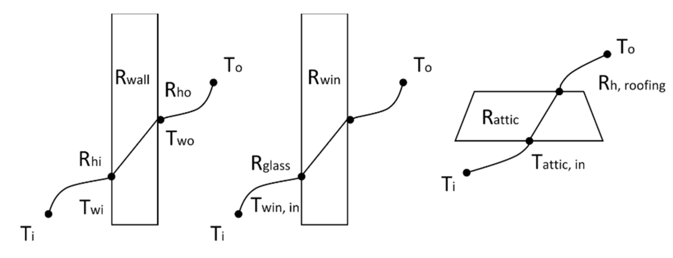
In order to estimate the MRT of a space, the interior temperature of all surfaces enclosing a space is needed. Non-exterior connected surfaces can be estimated to be equal in temperature to the room temperature, which is assumed to be adequately reflected by the measured smart WiFi thermostat temperature. The interior surfaces connected to exterior walls, ceiling, or basement/crawlspace are estimated from knowledge of the real-time room and exterior temperatures and envelope R-values. These temperatures are obtained using a steady-state heat transfer analysis. Application of an energy balance on each exterior connected surface under this assumption, and assuming that the solar gain on any of the surfaces is small, requires that the heat flow through the envelope component be equal to the heat flow from the interior surface of the envelope to the indoor air, as given by Equation (1) and shown in Figure 1.
where
- Rho = convective thermal resistance on exterior surface, typically 0.03 m2—C°/W.
- Rhi = convective thermal resistance on interior surface, typically 0.12 m2—C°/W.
- Re = conductive thermal resistance through envelope component.
- Te,in = interior surface temperature of envelope component.
Rearranging yields the following interior surface temperature of wall, given by
With all surface area information available through a home automation setup by the resident, and with estimates of the exterior envelope component interior surface temperatures, the MRT can be calculated using an area weighted average given by Equation (3).
3.3. Applying Thermal Comfort Control to WiFi Thermostats
A feedback control scenario based upon Fanger’s PMV equation [6], shown in Equation (4) below, was used to control the thermal comfort to be set as the minimum thermal comfort range for cooling. At each sampled time, the PMV was calculated based upon thermostat measurements (room temperature and humidity), and inferred thermostat measurement (MRT) and minimum thermal comfort values for other parameters in Fanger’s equation for the room air velocity, clothing level (Clo), and metabolic rate (MET).
Then the measured PMV was compared to the desired PMV and adjustments were made to the thermostat setpoint level if needed. The control logic was as follows. The thermostat setpoint value was increased/decreased by 1 degree if the PMV value was above 0.5 (minimum cooling thermal comfort condition) and less than 0; otherwise, the setpoint temperature was maintained.
This same logic would apply to a heating situation, except instead, the PMV would be maintained between −0.5 and 0 for minimum thermal comfort.
3.4. Smart Home Automation Assistant to Define Actual Minimum Thermal Comfort in A Residence
This research also considers the idea that the minimum comfort within a residence depends upon where the residents are. For example, if a resident is in a room with a large number of windows and with exposure to two or three exterior connected surfaces, the MRT could be much closer to the outdoor temperature than were a resident or residents in a room with little or no exposure to exterior walls, windows or attic walls. Thus, the determination of the minimum thermal comfort condition in a house should take into account where the residents are within a residence.
In a smart home automation era, it is feasible to know where people are in the residence. All a resident would need to do is say “John is in the living room” or “Sarah is in the dining room” to enable the automation system to know where they are located. Moreover, we could readily imagine an app that helps residents “set-up” their houses. They could identify for each room the following: the room dimensions, which walls are exterior walls, if the room is exposed to the attic space or roof, the number and size of windows in the room, and if the room’s floor is exposed to an unheated/uncooled space beneath.
Moreover, residents could even say what they are doing in each room, whether they are sitting, sleeping, exercising, or other things. Thus it would be feasible to more accurately estimate the metabolic level (MET). Lastly, they could also identify what clothing they are wearing and if they have an open window or a floor or ceiling fan. Thus, the CLO and vair parameters could theoretically be estimated with greater accuracy.
It will thus be possible to estimate the MRT and PMV real-time in each room. Knowledge of where occupants are will enable estimation of a worst-case PMV for the residence. The thermostat setpoint for a single zoned residence could then be adjusted to maintain a minimum comfort PMV in the worst-case occupied zone.
3.5. Assessing the Energy Savings Impact of Minimum Thermal Comfort Control Via Simulation
In this section, we describe a dynamic data-based model used to evaluate the energy-savings impact of the thermal comfort control strategy described in Section 3.3. The developed dynamic model leverages thermostat data for an individual residence, synched with simultaneous weather data. The thermostat data include human times, cool/heat/fan status, cooling/heating setpoint, indoor air temperature, and relative humidity, and outdoor weather conditions.
With the dynamic model developed for a residence, new setpoint targets based upon real-time PMV comfort assurance can be tested, and the resulting cooling (and heating) energy savings can be estimated.
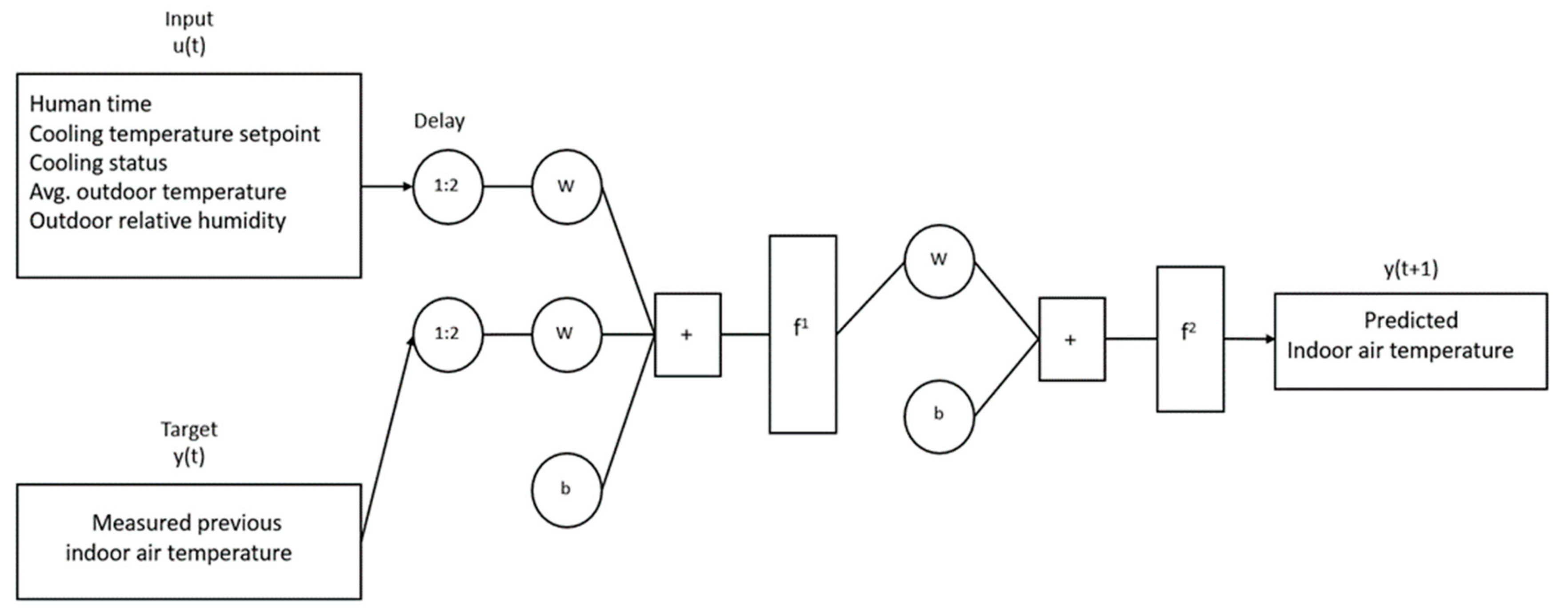
The dynamic model was developed based on a nonlinear autoregressive network with exogenous inputs (NARX) neural network. Figure 2 depicts this approach. The NARX was created in MATLAB 2019a, with 20 hidden neurons and the Levenberg–Marquardt as the training function.
Model validation was achieved by applying the model to data not used for the model training. The validation data inputs were outdoor temperature and humidity and interior thermostat setpoint data. The model was applied to predict indoor temperature and humidity. The predictions for these were compared to the measured values for those inputs in order to assess the efficacy of the developed model. R-squared and RMSE metrics were used to evaluate the quality of the validation.
4. Results
4.1. Case Studies
In this study, we considered smaller two story residences with floor areas of approximately 100 m2. Residences had 3 bedrooms, a living room, a dining room, a family room and a kitchen. Typical room dimensions in these residences are listed in Table 3 below (dimensions in meters).
In order to assess the variability of thermal comfort from room to room, we additionally considered variation in terms of exterior surface connection for the rooms themselves. Table 4 describes the two cases considered for each room. Case 1 for each room was associated with more interior surfaces being exposed to exterior surfaces. Case 2 was associated with less exterior surface connection. The floor condition for all cases was a conditioned full-basement. Thus, the floor surface was assumed to be at the residential ambient temperature in the calculation of the MET.
Lastly, in order to assess the effect of general residential energy effectiveness on thermal comfort control, particularly in terms of insulation, two general types of residences were studied: an energy-efficient one and an energy-inefficient one. Table 5 shows the wall, window, and attic RSI values (R-value in imperial units) employed in these two types of residences.
4.2. NARX Dynamic Model Performance
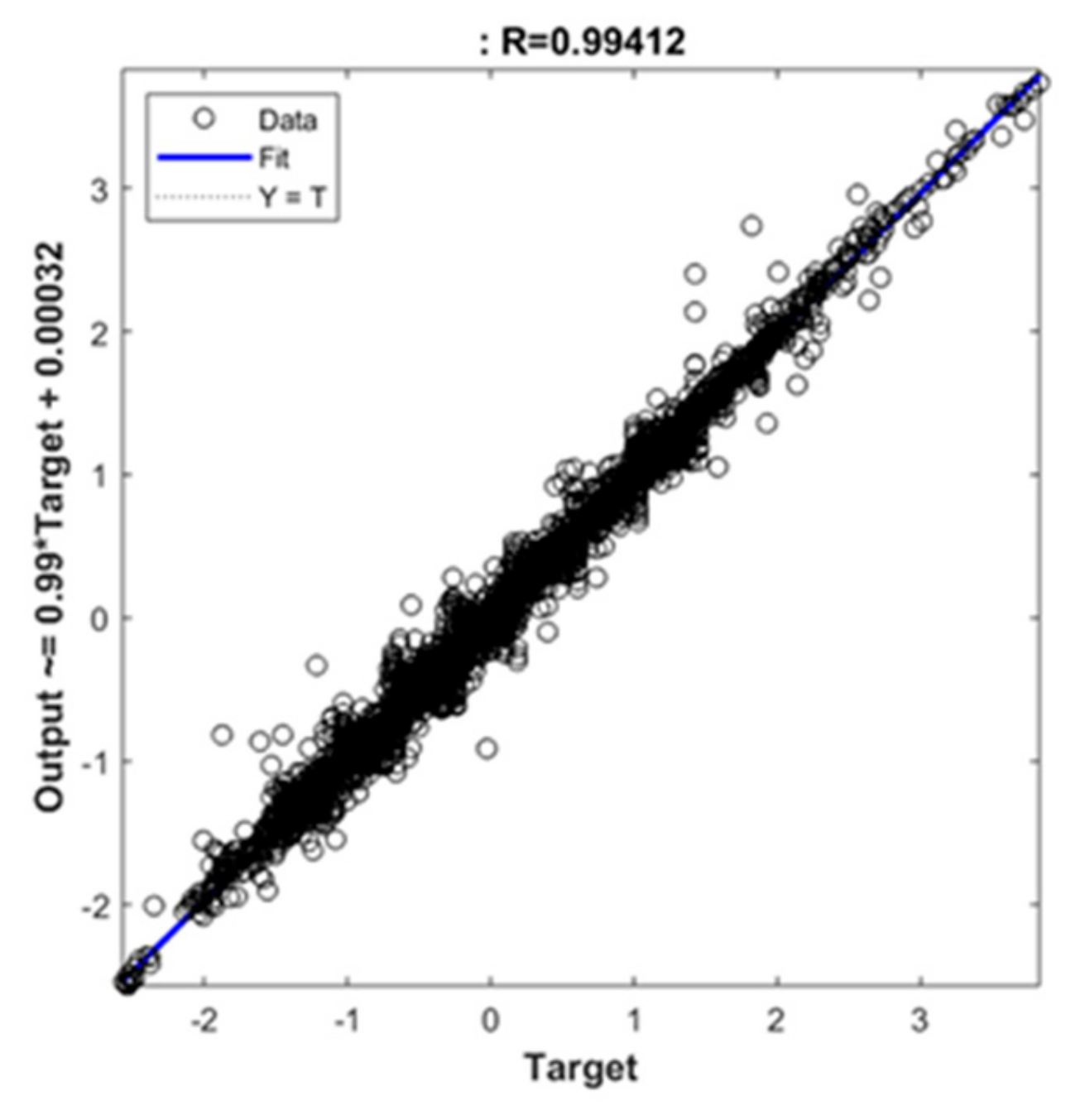
The suitability of the NARX model in predicting the temperature and humidity inside the residence, as estimated by the measured temperature and humidity at the thermostat, was validated. Figure 3 shows a plot of the predicted normalized temperature in the room versus the validated temperature for a high-efficiency residence. This plot illustrates a strong correspondence between the model prediction and the measured temperature. Similar results were seen for the low-efficiency residence case. The model validation metrics for the models developed were exceptional, with R-squared values for all developed models greater than 0.99.
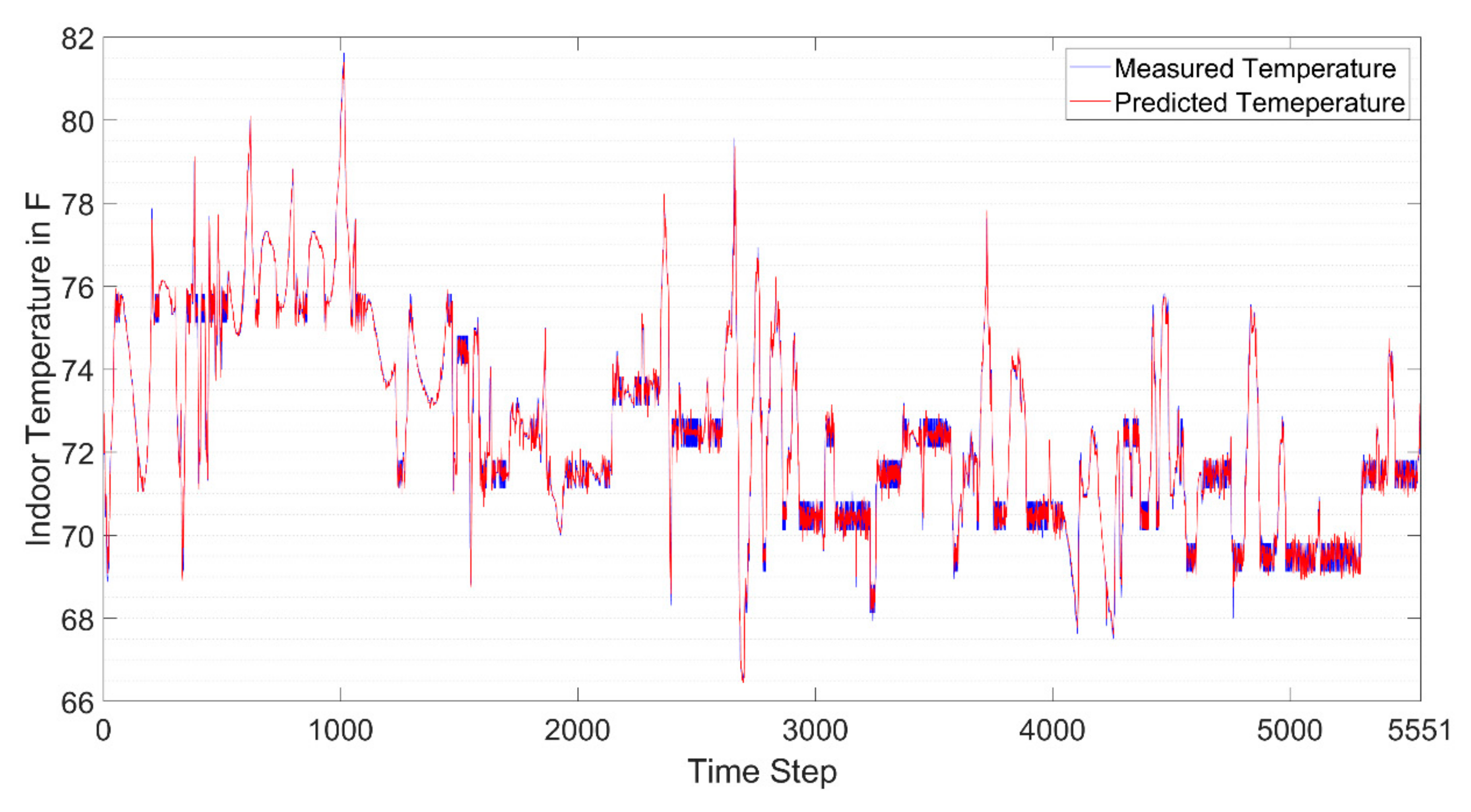
Figure 4 shows a time series plot of both the predicted and measured internal temperature for validation data; e.g., data not used to train the model. The plot again shows excellent correspondence between the two data series.
4.3. Effect of More Accurate Evaluation of MRT from Thermostat Data on the Indicated PMV in a Room
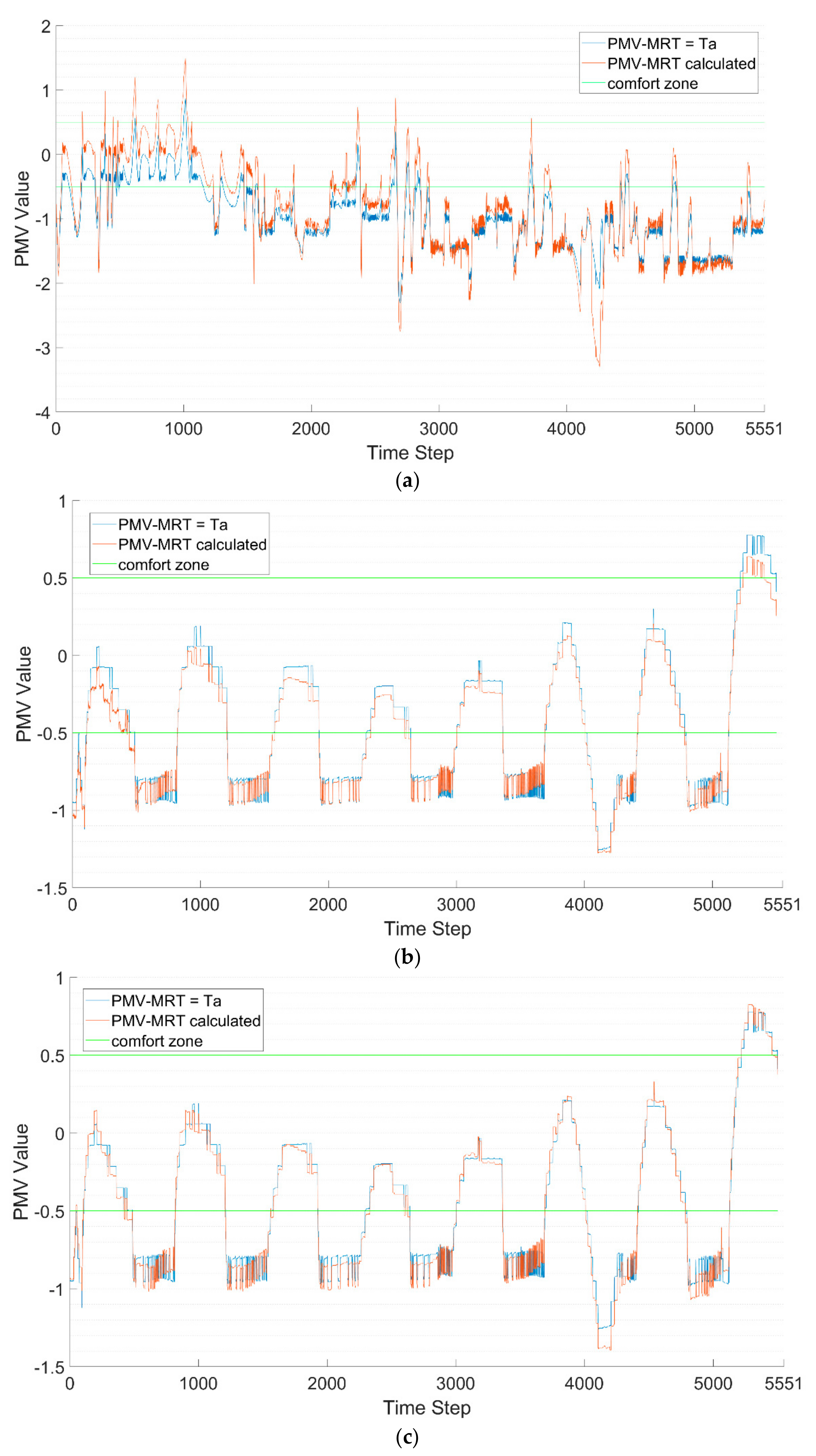
Comparative results are presented for the calculated PMV for non-thermal comfort controlled actual residential data using the standard MRT approximation as equal to the ambient temperature and the more accurate smart WiFi thermostat enabled MRT estimation posed herein. Figure 5a shows the PMV values in an efficient residence in a room with little exterior exposure calculated with the thermostat-enabled improved MRT in orange and the standard MRT in blue. Additionally, the thermal comfort zone, defined by ASHRAE 55, is represented by the region between two green lines. Here the assumed air flow is 0.1 m/s, the people in the space are sedentary, and have clothing levels of 0.36 (typical summer indoor clothing). It is shown that for this case there is little difference between the PMV determined from the two MRT methodologies. A similar result was observed for a room with significant exterior exposure.
Figure 5b,c, which shows the PMV values in an inefficient residence with, respectively, little and significant exterior exposure, shows a significant deviation between the calculated PMV using the new and standard MRT estimations. This is particularly true in Figure 5c, where significant exterior exposure causes greater thermal discomfort than predicted using the standard MRT estimation.
4.4. Simulation of Thermal Comfort Control
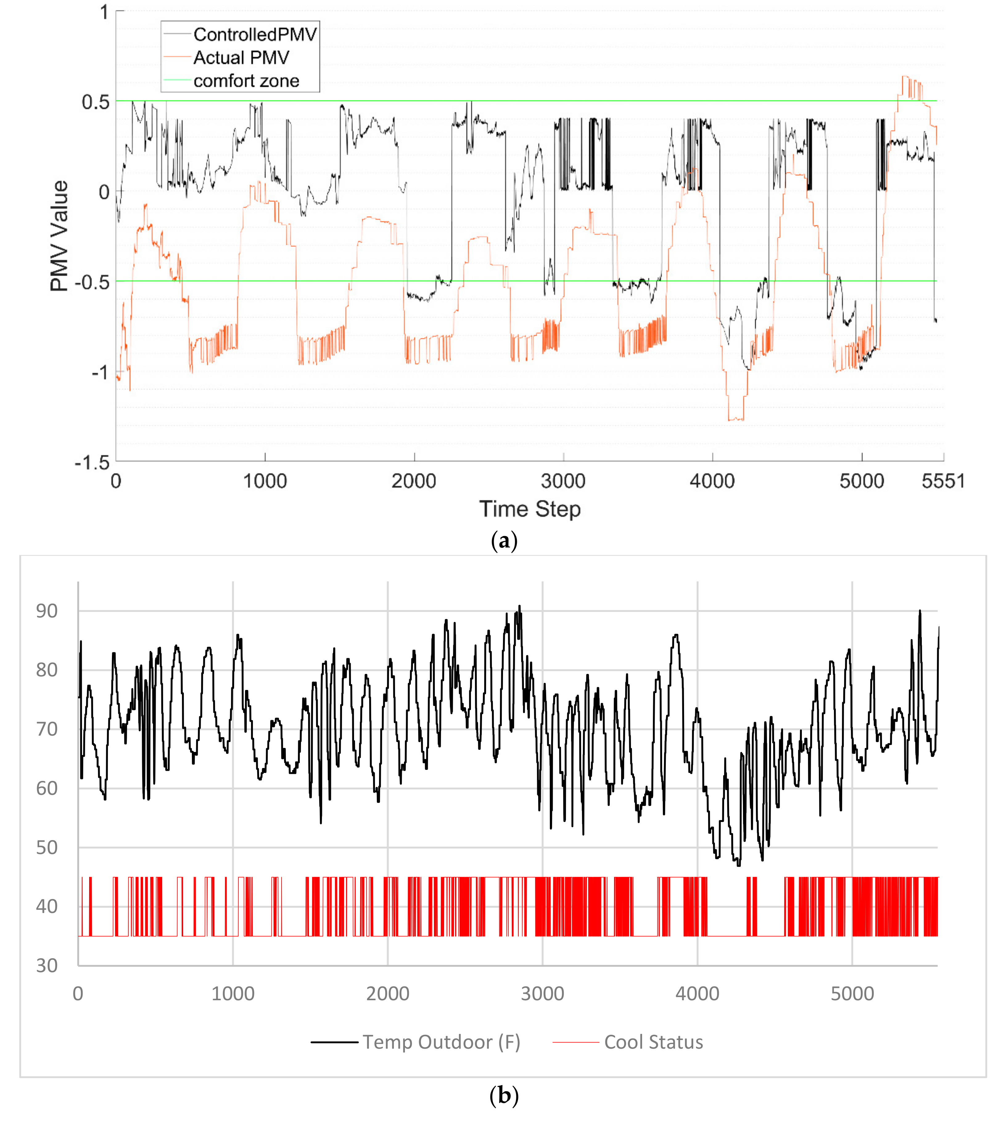
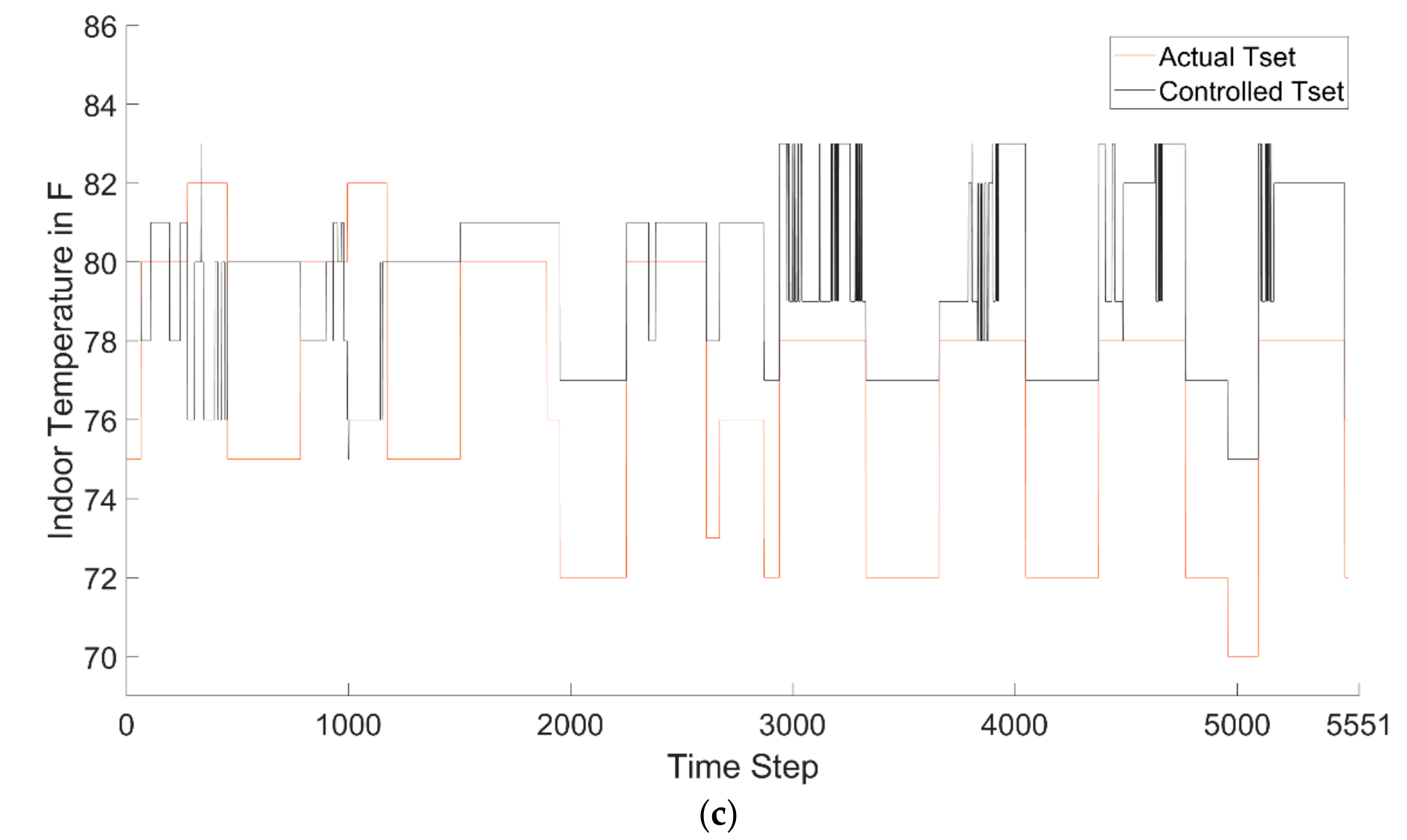
Figure 6 shows data and results from a simulation of thermal comfort control using the dynamic models for room temperature and humidity for a low-efficiency residence. Figure 6a shows the non-controlled outdoor temperature in degrees Fahrenheit and the cooling status (on or off) as a function of time. This plot shows that the cooling duty cycle is high for this period of time. Figure 6b shows the controlled PMV versus the actual non-controlled PMV associated with the case shown in Figure 5c (low-efficiency residence with large surface exposure). In this plot, it is clear that the PMV index is generally maintained within the desired PMV band from 0 to 0.5 using the posited control methodology, except where the outdoor temperature has dropped below the cooling setpoint and cooling is not needed. Figure 6c shows a time series of the setpoint condition established to maintain the desired PMV level in comparison to the actual setpoint for the non-controlled case. It is evident from this figure that a much higher temperature setpoint can be maintained in general to achieve the minimum thermal comfort condition desired. Thus, substantial energy savings are derived.
4.5. Energy Savings Based on Minimum Comfort in Individual Room
To estimate the cooling energy savings derived from minimum thermal comfort control, thermal control simulations such as those described in the previous section, which utilize the dynamic model developed for each residence applied to historical weather data, must be completed. From these simulations, the air conditioner system’s run time using thermal comfort control can be determined. Energy savings are then determined by calculating the difference between the actual and simulated cooling system’s run times.
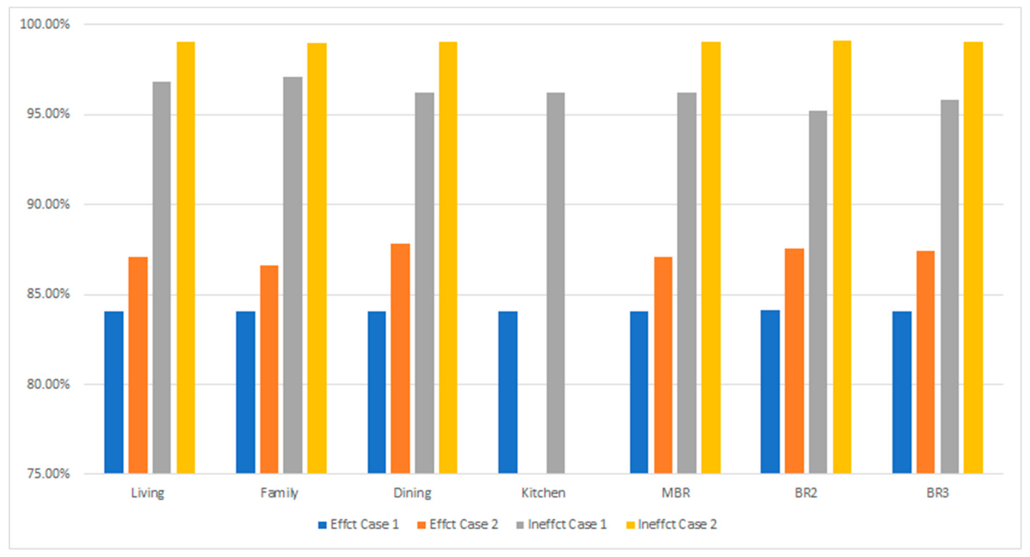
Figure 7 below shows the percentage cooling savings realized from minimum thermal comfort control for the different residential energy effectiveness and room exterior cases considered and for the different rooms described in Table 3, Table 4 and Table 5. The cases shown represent efficient and inefficient residences of equal size. For each room, two cases are shown; one representing a room with significant exterior surface (wall, window, or ceiling) exposure and another with little exterior surface exposure. The blue and grey bars are associated with significant exterior surface connection and the orange and yellow bars are associated with little exterior surface connection. Cooling energy savings relative to no PMV control were, respectively, in the range of 83%–87% for the efficient residential case and above 95% for the inefficient residential case. The savings were slightly less when there was more surface exposure because of a higher MRT, which requires establishment of a lower setpoint temperature in order to maintain minimum thermal comfort. Overall, these results show the potential value of integrating thermal comfort control into home automation systems. For example, if, for the cases considered, the home automation system knew that residents were all in the family room, a higher temperature setpoint could be maintained in order to insure minimum thermal comfort. Even greater savings are potentially derivable from this knowledge.
5. Conclusions
Implementation of a thermal comfort control which relies on a smart WiFi thermostat alone has been demonstrated. In this approach, an improved means to estimate the MRT, based upon prior estimation of exterior wall and ceiling RSI values obtained from smart WiFi thermostat information, was posed. The modified MRT estimation was shown to be particularly valuable in poorly insulated residences, especially if a space has a significant exterior connection.
Additionally, we demonstrated the ability to leverage a dynamic machine learning-based predictive model of the residential temperature and humidity measured by a smart WiFi thermostat using historical thermostat and outdoor weather data to estimate savings with thermal comfort control. Such models are derivable for any smart WiFi-equipped residence. Thus, we have demonstrated the ability to estimate thermal comfort control savings in any residence. This information could be communicated to occupants to enable them to choose to control for comfort rather than temperature alone.
Lastly, through simulated implementation of thermal comfort control using the developed dynamic models in both high- and low-efficiency residences, we have shown potential cooling savings for these types of residences to be, respectively, in the order of 85% and 95%. These results show the promise of smart WiFi thermostats enable thermal comfort control for achieving large scale savings from cooling. This research also reveals the opportunity to leverage home automation systems to permit thermal comfort control based upon the room or rooms where people are present.
The limitation of this research is that these conclusions have been drawn via simulations leveraging developed dynamic models of internal temperature and humidity in residences in order to assess the impact of thermal comfort control using a smart WiFi thermostat controller. Future research is needed to experimentally validate the savings from thermal comfort control in a variety of residences. As well, future research should explore the potential for integrating this type of control into home automation systems to enable room by room estimations of thermal comfort.
Author Contributions
Conceptualization, R.L. and K.P.H.; methodology, R.L., K.P.H. and T.R.; software, R.L. and K.H. validation, R.L. and K.P.H.; formal analysis, R.L.; investigation, R.L. and K.H.; resources, K.P.H. and T.R.; data curation, K.P.H.; writing—original draft preparation, R.L.; writing—review and editing, K.P.H. and T.R.; visualization, R.L.; supervision, K.P.H. and T.R.; project administration, K.P.H.. All authors have read and agreed to the published version of the manuscript.
Funding
This research is internally funded.
Acknowledgments
Emerson Sensi is acknowledged for their permission to access smart WiFi data for the housing set considered in this study.
Conflicts of Interest
The authors declare no conflict of interest.
References
- NEEP Energy. Opportunities for Home Energy Management Systems (HEMS) in Advancing Residential Energy Efficiency. Issuu. Available online: issuu.com/neepenergy/docs/2015_hems_research_report (accessed on 2 March 2020).
- Bonneville Power Administration. Smart Thermostats Market Characterization. 2018. Available online: https://www.bpa.gov/EE/Utility/Momentum-Savings/Documents/181016_BPA_Smart_Thermostats_Market_Characterization (accessed on 2 March 2020).
- Hansen, S.J. Managing Indoor Air Quality; Fairmont Press: Lilburn, GA, USA, 2011; pp. 149–151. ISBN 9780881736618. [Google Scholar]
- Kolokotsa, D.; Tsiavos, D.; Stavrakakis, G.S.; Kalaitzakis, K.; Antonidakis, E. Advanced fuzzy logic controllers design and evaluation for buildings’ occupants thermal-visual comfort and indoor air quality satisfaction. Energy Build. 2001, 33, 31–543. [Google Scholar] [CrossRef]
- Zhao, Q.; Cheng, Z.; Wang, F.; Jiang, Y.; Ding, J. Experimental study of group thermal comfort model. In Proceedings of the 2014 IEEE International Conference on Automation Science and Engineering (CASE), Taipei, Taiwan, 18–22 August 2014; pp. 1075–1078. [Google Scholar]
- Fanger, P.O. Thermal Comfort: Analysis and Applications in Environmental Engineering; McGraw-Hill: New York, NY, USA, 1970. [Google Scholar]
- Chaudhuri, T.; Soh, Y.C.; Bose, S.; Xie, L.; Li, H. On assuming Mean Radiant Temperature equal to Air Temperature during PMV-based Thermal Comfort Study in Air-conditioned Buildings. In Proceedings of the IECON 2016-42nd Annual Conference of the IEEE Industrial Electronics Society, Florence, Italy, 23–26 October 2016. [Google Scholar] [CrossRef]
- ASHRAE. Thermal Environmental Conditions for Human Occupancy; ASHRAE: Atlanta, GA, USA, 2004; Volume 55. [Google Scholar]
- ASHRAE. Addendum a to Standard 55-2013; ASHRAE: Atlanta, GA, USA, 2014. [Google Scholar]
- Dounis, A.I.; Tiropanis, P.; Argiriou, A.; Diamantis, A. Intelligent control system for reconciliation of the energy savings with comfort in buildings using soft computing techniques. Energy Build. 2011, 43, 66–74. [Google Scholar] [CrossRef]
- Ferreira, P.M.; Ruano, A.E.; Silva, S.; Conceição, E.Z.E. Neural networks based predictive control for thermal comfort and energy savings in public buildings. Energy Build. 2012, 55, 238–251. [Google Scholar] [CrossRef] [Green Version]
- Torres, J.L.; Martin, M.L.; Adaptive Control of Thermal Comfort Using Neural Networks. In Argentine Symposium on Computing Technology; 2008. Available online: https://www.researchgate.net/profile/Marcelo_Martin2/publication/268274253_Adaptive_Control_of_Thermal_Comfort_Using_Neural_Networks/links/54f713960cf28d6dec9d3616/Adaptive-Control-of-Thermal-Comfort-Using-Neural-Networks.pdf. (accessed on 2 March 2020).
- Ferreira, A.A.; Ludermir, T.B.; Aquino, R. Comparing recurrent networks for time-series forecasting. In Proceedings of the 2012 International Joint Conference on Neural Networks (IJCNN), Brisbane, Australia, 10–15 January 2012. [Google Scholar]
- Deng, Z.; Chen, Q. Artificial neural network models using thermal sensations and occupants’ behavior for predicting thermal comfort. Energy Build. 2018, 174, 587–602. [Google Scholar] [CrossRef]
- Ciabattoni, L.; Cimini, G.; Ferracuti, F.; Grisostomi, M.; Ippoliti, G.; Pirro, M. Indoor thermal comfort control through fuzzy logic PMV optimization. In Proceedings of the 2015 International Joint Conference on Neural Networks (IJCNN), Killarney, Ireland, 12–17 July 2015; pp. 1–6. [Google Scholar] [CrossRef]
- Marvuglia, A.; Messineo, A.; Nicolosi, G. Coupling a neural network temperature predictor and a fuzzy logic controller to perform thermal comfort regulation in an office building. Build. Environ. 2014, 72, 287–299. [Google Scholar] [CrossRef]
- Alanezi, A.; Huang, K.; Hallinan, K.P.; University of Dayton, Dayton, OH, USA. Personal Communication, 2018.
- NOAA’s Climate Divisional Database (NCLIMDIV). Data.gov, Responsible Party DOC/NOAA/NESDIS/NCEI > National Centers for Environmental Information, NESDIS, NOAA, U.S. Department of Commerce (Point of Contact), 27 February 2019. Available online: catalog.data.gov/dataset/noaas-climate-divisional-database-nclimdiv (accessed on 2 March 2020).
Figure 1.
Thermal resistance analysis of heat flow through envelope components.

Figure 2.
NARX architecture used to predict the indoor temperature. The model uses synched smart WiFi and weather data.
Figure 2.
NARX architecture used to predict the indoor temperature. The model uses synched smart WiFi and weather data.

Figure 3.
Predicted versus actual temperature validation data, not used to develop model, for high-efficiency residences
Figure 3.
Predicted versus actual temperature validation data, not used to develop model, for high-efficiency residences

Figure 4.
Time series plot for predicted (red) and actual (blue) measured indoor temperature as a function of time for a high-efficiency house case and no external surface exposure
Figure 4.
Time series plot for predicted (red) and actual (blue) measured indoor temperature as a function of time for a high-efficiency house case and no external surface exposure

Figure 5.
Thermal comfort simulation result: the PMV value with calculated MRT versus the ASHRAE standard MRT for (a) high-efficiency residence in a room with little exterior exposure; (b) low-efficiency residence with little exterior exposure; and (c) low-efficiency residence with significant exterior exposure.

Figure 6.
Thermal comfort control in a low-efficiency residence with significant room exterior exposure plots documenting the (a) baseline time series for the outdoor temperature and non-controlled cooling status; (b) PMV time series from thermal comfort control in comparison to no control; and (c) temperature setpoint time-series comparisons of the actual thermostat setpoint and the thermostat setpoint required to maintain the PMV in the range of 0 to 0.5.


Figure 7.
Percentage cooling energy savings using minimum thermal comfort control for both an efficient and inefficient residence for various rooms with significant (blue and grey) and little exterior surface connection (orange and yellow).
Figure 7.
Percentage cooling energy savings using minimum thermal comfort control for both an efficient and inefficient residence for various rooms with significant (blue and grey) and little exterior surface connection (orange and yellow).


Table 1.
Fanger’s PMV level values and associated thermal sensation.
| Value | Sensation |
|---|---|
| +3 | Hot |
| +2 | Warm |
| +1 | Slightly warm |
| 0 | Neutral |
| −1 | Slightly cool |
| −2 | Cool |
| −3 | Cold |
Table 2.
Summary of calculation of MRT for use in thermal comfort calculations.
| Author (Year) | MRT | Thermal Comfort Assessment | Assumed Factors | Control Technique | Energy Savings | Sensors/Other Hardware |
|---|---|---|---|---|---|---|
| Torres et al. (2008) [12] | Suggested consideration of thermal radiation to/from walls; however, no clear method described | Standard Fanger’s PMV formulation | Clothing = 0.6–0.8 Clo (summer) Airflow = 0.1 m/s MET = 1–1.7 | NN based on PMV index to control setpoint through a PI controller | Not directly measured | Not mentioned |
| Ferreira et al (2012) [13] | Measured by room-based thermometer | Standard Fanger’s PMV formulation | Clothing = 0.65–1.0 Clo (summer) Air flow = 0.08–0.1 m/s MET = 1 | Models developed to predict indoor temperature and PMV. Used in model predictive control bounded by PMV | 41%–77% compared to traditional controls | Significant use of additional sensors |
| Zheng et al. (2018) [14] | Assumed equal to room air temperature | From occupant surveys | Clothing level obtained by questionnaire Airflow <0.2 m/s MET = 1 | No control. Merely assessed thermal comfort | NA | Thermostat, building automation system, data logger |
| Ciabattoni et al. (2015) [15] | Assumed equal to room air temperature | Standard Fanger’s PMV formulation | Clothing = 0.65 Clo Airflow = 0.2 m/s MET = 1 | FLC used to control fan speed | Not mentioned | Humidity and temperature sensors with EnOcean technology |
| Marvuglia et al. (2014) [16] | Assumed equal to room air temperature | Not directly addressed | Not mentioned | Coupled NARX/FLC controller | Not mentioned | Air temperature airspeed data logger |
Table 3.
Typical room dimensions in residences considered in the study
| Living room 3.7 × 5.5 | Dining room 3.4 × 3.7 | Family room 3.7 × 4.9 |
| Kitchen 3 × 3 | Bedroom 3.4 × 3.4 | Master bedroom 3.7 × 4.6 |
Table 4.
Types of rooms considered with two different cases of exterior surface connection.
| Room Name | Case 1—Significant Exterior Connection | Case 2—Little Exterior Connection |
|---|---|---|
| Living room | 2 exterior walls, 2 windows, ceiling, 1st floor | 1 exterior wall, no window, ceiling, 1st floor |
| Family room | 2 exterior walls, 4 windows, ceiling, 1st floor | 1 exterior wall, 1 window, ceiling, 1st floor |
| Dining room | 2 exterior walls, 2 windows, ceiling, 1st floor | 1 exterior wall, no window, ceiling, 1st floor |
| Kitchen | 1 exterior wall, 1 window, ceiling, 1st floor | N/A |
| Master bedroom | 2 exterior walls, 2 windows, ceiling (attic), 2nd floor | 1 exterior wall, 1 window ceiling (attic), 2nd floor |
| Bedroom 2 | 2 exterior walls, 2 windows, ceiling (attic), 2nd floor | 1 exterior wall, 1 window, ceiling (attic), 2nd floor |
| Bedroom 3 | 2 exterior walls, 2 windows, ceiling (attic), 2nd floor | 1 exterior wall, 1 window, ceiling (attic), 2nd floor |
Table 5.
RSI value of inefficient and efficient building envelope.
| Envelope RSI Value | Inefficient Residence | Efficient Residence |
|---|---|---|
| RSIwall | 0.88 | 2.47 |
| RSIwindow | 0.18 | 0.35 |
| RSIattic | 1.06 | 5.28 |
© 2020 by the authors. Licensee MDPI, Basel, Switzerland. This article is an open access article distributed under the terms and conditions of the Creative Commons Attribution (CC BY) license (http://creativecommons.org/licenses/by/4.0/).
Share and Cite
MDPI and ACS Style
Lou, R.; Hallinan, K.P.; Huang, K.; Reissman, T. Smart Wifi Thermostat-Enabled Thermal Comfort Control in Residences. Sustainability 2020, 12, 1919. https://doi.org/10.3390/su12051919
AMA Style
Lou R, Hallinan KP, Huang K, Reissman T. Smart Wifi Thermostat-Enabled Thermal Comfort Control in Residences. Sustainability. 2020; 12(5):1919. https://doi.org/10.3390/su12051919
Chicago/Turabian StyleLou, Robert, Kevin P. Hallinan, Kefan Huang, and Timothy Reissman. 2020. "Smart Wifi Thermostat-Enabled Thermal Comfort Control in Residences" Sustainability 12, no. 5: 1919. https://doi.org/10.3390/su12051919
Note that from the first issue of 2016, this journal uses article numbers instead of page numbers. See further details here.