The Effect of Globalization on Economic Development Indicators: An Inter-Regional Approach


Departamento de Economía y Empresa, Universidad de Almería, 04120 Almería, Spain
*
Author to whom correspondence should be addressed.
Sustainability 2020, 12(5), 1942; https://doi.org/10.3390/su12051942
Submission received: 18 November 2019
/
Revised: 27 February 2020
/
Accepted: 29 February 2020
/
Published: 3 March 2020
(This article belongs to the Special Issue Local and Regional Development in the Conditions of Globalisation)
Abstract
:Background: The analysis of the problems derived from globalization has become one of the most densely studied topics at the beginning of this millennium, as they can have a crucial impact on present and future sustainable development. This paper analyzes the differential patterns of globalization in four worldwide areas predefined by The World Bank (namely, High-, Upper-Middle-, Lower-Middle-, and Low-Income countries). The main objective of this work is to estimate the effect of globalization on some economic development indicators (specifically per capita income and public expenditure on health) in 217 countries over the period 2000–2016. Methods: Our empirical approach is based on the implementation of a novel econometric methodology: The so-called Toda–Yamamoto procedure, which has been used to analyze the possible causal relationships between the involved variables. We employ World Development Indicators, provided by The World Bank, and the KOF Globalization Index, elaborated by the KOF Swiss Economic Institute. Results: The results show that there is a causal relationship in the sense of Granger between globalization and public expenditure on health, except in High-Income countries. This can be interpreted both negatively and positively, confirming the double character of globalization, as indicated by Stiglitz.
1. Introduction
At the end of the 1970s of the last century, Krugman [1] warned of the advent of a new economic phenomenon, the so-called globalization, which, if due measures were not taken, would sooner or later end up dominating the international economic concert, as finally happened. This process would soon transcend the economic field to become a multidimensional phenomenon [2], annexed to subjectivity and, therefore, difficult to analyze objectively. Usually, globalization does not highlight its “neutral” nature [3], but mainly its negative externalities [4], bypassing the positive externalities [5]. Additionally, globalization plays a leading role as an amplifying element that would contribute to further increase of socio-economic inequalities between different countries and international areas.
This paper, inspired by the New Economic Geography [1,6,7], responds to the need to analyze globalization objectively by considering it, according to the cumulative causation described by Myrdal [8], as a “concatenation of causal relationships”. Moreover, it studies the evolution of globalization in four worldwide inter-regional areas predefined by The World Bank in terms of per capita income and according to the Atlas methodology [9]. The KOF Globalization Index, provided by the KOF Swiss Economic Institute [10], and two variables (per capita income and per capita public spending on health) intrinsically related to globalization have served to perform a causal analysis by implementing the Toda–Yamamoto [11] procedure throughout the period 2000–2016, with data obtained from The World Bank (World Development Indicators) [12].
Based on this econometric test, implemented in four worldwide inter-regional areas (High, Upper-Middle, Lower-Middle, and Low Income countries), three types of causal relationships have been detected. Indeed, given the externalities always associated to the globalization process, this can have both positive [13] and negative repercussions [4].
This paper has been structured as follows. Section 2 presents a literature review of the main empirical approaches to globalization, taking into account its relationship with the New Economic Geography. Section 3 describes the data and the methodology. This section also contextualizes, at an exploratory level, the four analyzed global areas and the nature of the variables implemented in the empirical analysis based on the Toda–Yamamoto methodology. Section 4 presents the results derived after applying this methodology. Finally, Section 5 includes the discussion, and Section 6 summarizes and concludes.
2. Literature Review
2.1. Globalization
Globalization is a “complex and multifaceted” phenomenon [14] which has a permanent influence on world economies, increasingly integrated and open to the exterior [15]. Consequently, the limits of the economies are no longer their transnational borders, but the whole world itself.
In practice, for [16], globalization supposes the creation of a transnational single market guided by the principles of free trading and enhanced by dynamic flows of exchange of information, which offers the opportunity for organizations and individuals to carry out practically any kind of economic transaction, without having to be subordinated to national borders.
The hypothesis of globalization could be explained by the so-called New Economic Geography (hereinafter, NEG) by Krugman [3,6,7]. In effect, the classical macroeconomic model ignores some concepts such as the distances between the production centers based in different countries and geographical areas, the level of transport costs, or “space” as a key magnitude for the analysis of internationalized economies. Krugman’s approach is completely different from the classical approach because, independently of the considered degree of openness of the economies, the traditional approach does not take into account the impact of economic globalization.
According to [17], the NEG is a theory of the emergence of large agglomerations, based on the analysis of increasing returns to scale and transport costs by fundamentally studying the links between transnational companies and suppliers. Mainly the reduction of transport costs would validate the initial assumptions of globalization [1,18], given that this reduction allowed the intensification of the increasing returns to manufacturing scale, encouraging the geographical concentration of the production of each good.
The NEG [19], in addition to verifying these initial hypotheses about globalization, establishes a very adequate analytical formulation of so-called Space Economics at the level of countries and geographical areas [20]. A first sketch of the effect of internationalization on a set of macroeconomic variables was pointed out by [21].
The approach of this paper is the causal analysis of globalization in relation to two noteworthy macroeconomic variables, viz. per capita income and government health expenditure. The choice of these variables is justified in the following two paragraphs.
2.1.1. Per Capita Income
The theoretical literature focused on the relationship between globalization and economic growth reports a contradictory discussion of this relationship. In this way, globalization is expected to have a positive effect on growth through the effective improvement of productivity factors and technology [22]. In contrast, according to [23], globalization does not incentivize economic growth because of its negative effects on job creation and on increase of risk. In addition, the authors of [24] argue that globalization has a negative effect on economic growth in countries with weak institutions and political instability.
On the other hand, there is a wide range of empirical literature about the above relationship (see Section 2.2). However, this study empirically examines the link between globalization and the level of per capita income, rather than focusing on the link between globalization and the economic growth effect.
2.1.2. Government Health Expenditure
Theoretically, globalization has also been analyzed as a phenomenon that can affect government size. In this way, there are two main hypotheses on the relationship between globalization and government expenditures. The first hypothesis, called the competition hypothesis, claims that governments are induced to diminish the sizes of public sectors via reducing expenditures and revenues (e.g., [25]). Oppositely, the second hypothesis, called the compensation hypothesis, states that globalization increases government expenditures in order to correct the adverse effects derived from the globalization process, such as inequality in income distribution (e.g., [26]).
There exists a large amount of empirical literature based on the potential link between globalization and the sizes of governments, the latter measured by government expenditure as a whole or welfare expenditures in particular (see Section 2.2). However, there is a gap in the literature particularly in the case of public health expenditure, one of the main components of welfare expenditure. From this perspective, public healthcare expenditure can be considered as a proxy of the size of a government and as an indicator of the social development of a country. In consequence, this study employs (considers) this type of public expenditure to test both the compensation and the competition hypotheses. In addition, we considered a broad sample of countries to include both countries that substantially subsidize health care and those that do not.
2.2. Empirical Literature Review
Many efforts have been made to empirically explain the association between globalization and other economic and social phenomena. Since globalization is a multifaceted process, the previous literature has analyzed whether globalization influences issues as different as labor market institutions [27], financial intermediation [28], inequality [29], human rights [30], and human development [31], among others.
From a macroeconomic perspective, a first group of empirical literature concentrates on the effect of globalization on economic growth and per capita gross domestic product (GDP). With regard to GDP growth, part of the previous research used five-year averages of per capita GDP growth to consider long-run GDP growth [32]. The author of [33] analyzes the nexus between the globalization index and five-year averages of per capita GDP growth by using data of 123 countries which cover the time period 1970–2000. The data are again five-year averages and cover the time period 1970–2004 for 122 countries in [34]. The authors of [35] examine the relationship between government size and economic growth in 29 OECD (Organisation for Economic Co-operation and Development) countries over the periods 1970–1995 and 1970–2005. The KOF index is used as an explanatory variable. Reference [36] investigates the nexus between government ideology and economic growth in a panel of 23 OECD countries over the period 1971–2004 and considers the overall KOF globalization index as control variable. The authors of [37] investigate the association between KOF globalization indices and economic growth in 101 developing and developed countries over the period 1970–2005. The authors of [38] extend this type of analysis to Singapore, Malaysia, Thailand, India, and the Philippines over the period 1974–2004. Reference [39] investigates the impact of globalization on economic growth in 21 low-income African countries. The authors of [40] analyze the influence of economic globalization and economic crisis on economic growth by employing data for 41 African countries over the period 1970–2009. The authors of [10] use the KOF globalization index to examine whether globalization promotes economic growth. Their sample includes 137 developed and developing countries over the period 1975–2010. They follow related studies, such as [33], and estimate the model based on five-year averages.
Other studies have employed annual GDP growth to consider how this variable is affected by globalization [41,42] or by other variables when globalization is included as an explanatory variable to overcome the bias by omission of variables [36,43]. The authors of [41] analyze the association between economic globalization and annual GDP growth in 189 countries over the period 1950–2009. Reference [42] examines how globalization and energy exports influence annual GDP growth in five South Caucasus countries between 1990 and 2009. On the other hand, Reference [36] investigates the influence of electoral cycles and government ideology on annual GDP growth in a panel of 23 OECD countries over the period 1971–2004, whilst Reference [43] examines the influence of political cycles in a panel of 21 OECD countries during the period 1971–2006.
Rather than focusing exclusively on average growth effects, other researches have concentrated on per capita GDP or income when studying the macroeconomic impact of globalization. The authors of [44] employ data for 23 OECD countries over the period 1970–2006 to investigate the influence of globalization indices on per capita GDP, whilst the authors of [45] use data for the G7 countries over the period 1970–2006. In a different region, Reference [46] extends this type of analysis to 31 Sub-Saharan African countries over the period 1980–2005. The authors of [47] examine the relationship between economic globalization and growth in a panel of selected Organization of Islamic Cooperation (OIC) countries over the period 1980–2008. Furthermore, these authors explore whether the growth effects of economic globalization depend on the set of complementary policies and income levels of OIC countries. The authors of [48] study economic globalization as a multidimensional process and investigate its effect on income in a panel of 147 countries during the period 1970–2014.
A second group of researches are concentrated on the relationship between globalization and size of government measured by government expenditures and revenues (for the latter case of public revenues, see [33,49,50,51]). Focusing on public expenditure, some researches consider the impact of globalization on overall government expenditure. The authors of [52] evaluate the relationship between globalization indices and overall public expenditure by using data of 186 countries from 1970 to 2004. The authors of [53] extend this type of analysis to a sample of 42 Sub-Saharan African countries in the period 1970–2009. Both of the above studies consider five-year averages. In other studies focused on evaluating political budget cycles, globalization is included as a control variable and fiscal policies are measured by the budget balance and total government expenditure in 65 democratic countries over the period 1970–2005 [54]. In addition, Reference [55] examines the fiscal performance under minority governments by using data on central and general governments of 23 OECD countries over the period 1960–2015. This study considers the “trade openness” (sum of imports and exports as a share of GDP) as an explanatory variable, as well as the KOF globalization index.
More specifically, part of the literature has concentrated on a specific government expenditure, such as social welfare expenditure. Reference [56] examines the impact of globalization on the social welfare expenditure in developed and developing countries during 1990–2003. References [57] and [51] study the correlation between globalization and social expenditure by using data of EU-27 countries over the period 1990–2006 and EU-15 countries over the period 1970–2007, respectively. Reference [58] investigates how government ideology is correlated with social expenditures, depending on whether globalization took place quickly or slowly, in a sample of 20 OECD countries from 1980 to 2003. On the contrary, globalization is incorporated as an explanatory variable when the authors of [59] investigate the relationship between social expenditure and international migration in 25 OECD countries in the period 1980–2008. Other functions of government expenditure have been taken into account in the studies based on the effects of globalization. The authors of [60] incorporate the globalization indices to investigate political cycles in social and military expenditures in 22 OECD countries from 1988 to 2009. The authors of [61] assess whether globalization was correlated with education expenditures in a sample of 104 countries over the period 1992–2006. These authors distinguish between expenditures for primary, secondary, and tertiary education. Reference [62] examines the relationship between economic growth, industrialization, urbanization, globalization, and population aging and the size of government health expenditure in 10 Association of Southeast Asian Nations (ASEAN) member countries from 2002 to 2011. In addition, the authors of [63] analyze whether globalization has indeed influenced the composition of government expenditures. They use a data set of the economic expenditure categories (capital expenditures, expenditures for goods and services, interest payments, subsidies, and other current transfers) for a sample of 60 countries during the period 1971–2001. Additionally, they employ data of some functions of government expenditures (defense, order, economic affairs, environment, housing, health, recreation, education, and social expenditures) for OECD countries.
Whilst previous literature has investigated the existence of a potential link between globalization and government expenditures, there is still a gap, particularly in the case of public health expenditures and this relationship with globalization. Therefore, the objective of this paper is to analyze the effect of globalization on public health expenditure and per capita income as measures of economic development indicators in 217 countries over the period 2000–2016.
3. Materials and Methods
3.1. Data
To carry out the empirical part of this work, the planet has been subdivided into four economic areas according to their corresponding categorizations relative to the level of income displayed in each specific area [64] according to the Atlas methodology established by The World Bank [9], as detailed in Table 1.
Specifically, this differentiation establishes four areas or worldwide subregions, as indicated in Figure 1: High-Income countries, Upper-Middle-Income countries, Lower-Middle-Income countries, and Low-Income countries (hereinafter, LI, UMI, LMI, and HI).
Having defined the period 2000–2016 as the time horizon to which the proposed causal analyzes are attached, the KOF index was chosen as a proxy variable for globalization (last index revision, see [10]). This index was used because it reflects the multidimensional nature of globalization through 43 variables structured in three differentiated dimensions: Economic, social, and political, distinguishing two fields in the conceptualization of economic globalization: Financial and exports, in addition to the following variables obtained from The World Bank database [12]: HEALTH (domestic general government health expenditure per capita—current US $) and INCOME (adjusted net national income per capita—current US $). The main descriptive statistics of the dataset, derived from the formerly defined variables KOF, HEALTH, and INCOME, over the period 2000–2016, are reported in Table 2. Since the variations of the INCOME variable (arithmetic terms) were used for the implementation of the causal analysis, the descriptive statistics have been delimited to the 2001–2016 period.
Among other conclusions, it can be inferred a priori that there would seem to be a direct relationship between the income level according to the Atlas methodology [12] and the globalization measured by the KOF index of each world area. It is necessary to remark on the inter-regional heterogeneity at the per capita income level with a substantial difference between two antagonistic poles, represented by the countries of the HI and LI areas, which, today, seems insurmountable in terms of real convergence. A similar consideration could be made of per capita public health expenditure, whose diagnosis seems to be equivalent to the previous one since, inexcusably, the material poverty of some regions (especially LI and LMI countries) limits the realization of extensive governmental efforts. This is necessary to cover the minimum vital needs in terms of health care or of establishing structures properly comparable to those of the Welfare State, capable of offering social services [65] in those nations established in areas whose purchasing power is extremely low.
The descriptive statistics (Table 2) offer a significant but eminently static picture of the four studied areas. Conversely, in Figure 2, we can observe a clorophet map which shows, individually and for all the nations of the planet (with the sole exceptions of South Sudan and Greenland), to what extent globalization, conceptualized according to the KOF index during the period 2000–2016, becomes itself the economic factor, without being the only one, which determines this phenomenon given its multidimensional character.
3.2. Methodology
The use of the KOF index as an objective measure of globalization presents enormous benefits for the analysis of this phenomenon, to such an extent that its representativeness has made it one of the standards of the empirical literature [32]. However, its implementation may present certain problems related to its robustness [66,67], a fact that, in any empirical analysis, can lead to the obtaining of regressions and causal inferences of a purely spurious nature. In this sense, Reference [32], based on [44,45,46,68,69], indicates that KOF indices exhibit a unit root, thus increasing the possibility of generating spurious regressions when both this index and any other variables jointly analyzed are not stationary. Obviously, these limitations are not exclusive to this particular index, since, in general terms, reaching spurious causal regressions and inferences may be due to other reasons, such as those indicated by [70,71] and, in particular, the presence of a “third confounding factor” (see, e.g., [72]). In any case, these reasons do not inhibit the performance of a rigorous causal analysis, such as that suggested by [32], taking into account the causal procedure by Toda–Yamamoto [11].
The Toda–Yamamoto procedure begins from the following premise: The implementation of the classic Granger Causality test [73] from a VAR (Vector AutoRegressive) model can lead to non-stationarity problems in the series, as it is necessary to confirm the type of existing cointegration [74]. The authors of [11,75] point out that the “conventional” Wald test produces integrated or cointegrated causal VAR models, which would inevitably lead to obtaining spurious Granger causality relationships [76]. However, the Toda–Yamamoto [11] procedure drastically avoids this handicap by developing a Modified Wald test (MWALD) for restrictions on the parameters of a VAR (p) model. This test is generated on a distribution, with (or number of time lags [77]). In Wolfe-Rufael’s words [78], the fundamental idea underlying this procedure is to “artificially augment the correct VAR order, p, by the maximal order of integration, say . Once this is done, a -th order of VAR is estimated and the coefficients of the last lagged vector are ignored” [79]. The resulting VAR model is formulated in Equations (1) and (2):
where and are the VAR error terms and is the maximum order of integration, according to the original specification of the Toda–Yamamoto procedure [11]. Therefore, in Equation (1), causality in the sense of Granger between X and Y will be detected, provided that for every i, and, on an identical basis, Equation (2) will imply causality in the sense of Granger between X and Y, if for every i.
Once the VAR model is obtained, the implementation of the Toda–Yamamoto [11] procedure in practice requires the realization of a series of steps [80], which Reference [74] summarizes in three differentiated steps: Testing each time-series to conclude the maximum order of integration of the variables by using, individually or jointly, the following tests: ADF (Augmented Dickey–Fuller) [81], KPSS (Kwiatkowski–Phillips–Schmidt–Shin) [82], and/or PPE (Phillips-Perron) [83]. Next, the optimal lag length (p) should be obtained based on the criteria: AIC (Akaike Information Criterion) [84], FPE (Akaike’s Final Prediction Error) [85], SC (Schwartz) [86], HQ (Hannan and Quinn) [87], and LR (Likelihood-Ratio) [88], seeking, as much as possible, an optimal length supported by the maximum degree of unanimity between criteria. Finally, the Granger causality test between the variables X and Y (in both directions) is properly performed by considering that the rejection of the null hypothesis implies the existence of causality in the sense of Granger according to the Toda–Yamamoto procedure [11] and that a reciprocal rejection would indicate a bilateral causal relationship between the analyzed variables.
4. Results
For the application of this procedure, the robustness of the series was estimated by using the ADF test [81]. Any of these constitutes one of the necessary tasks for implementing the Toda–Yamamoto procedure [11]. The results of these tests are summarized in Table 3.
Next, the following VAR models were generated for each differentiated area by applying an approach completely analogous to those of other works, such as [72,74,77,78,89,90,91,92]:
where the superscript variable, V, denotes the membership in each of the four areas analyzed, that is to say, V = HI, UMI, LMI, and LI. In the same way, the different null hypotheses were elaborated [74]:
Finally, Table 4 collects the causal analysis according with the four predefined areas:
Obviously, the fact of having a relatively reduced time horizon for the set of analyzed variables was due to the lack of available data that would have allowed a more robust analysis based on the different VAR models created. This methodology is especially suitable for the field of macroeconomics, which requires a high number of variables. This does not imply that it was specifically restricted to this specific area. With regard to the analysis carried out in this work, the use of a limited number of variables (small-dimension VAR), with the omission of any other important variable, can induce the detection of causality when, in purity, such causal relationships could be nonexistent. Another necessary consideration is to highlight the possibility that, given a VAR model, this could be affected by the so-called confounding variable, that is, an existing causal relationship between two variables that, in reality, is the result of the interaction of a third (see, e.g., [72]).
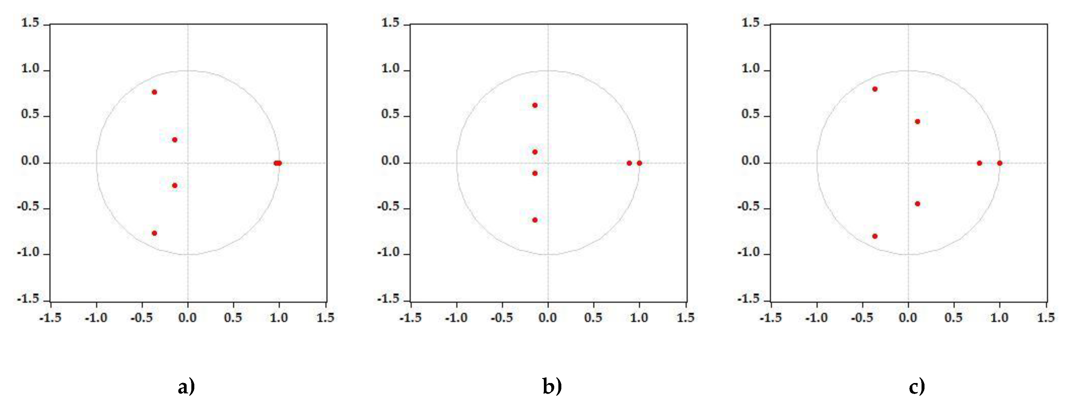
For these reasons, Figure 3, Figure 4, Figure 5 and Figure 6 show the stability of the parameters of the built VAR by analyzing them through the inverse roots of the characteristic AR (AutoRegressive) polynomial displayed in an Argand Diagram (or Argand Plane, see, e.g., [80]). According to this procedure, all of the points included in the circle determine a stable model. In this sense, all of the elaborated VAR models can be considered stable, with the exception of c) in the UMI and LI countries (Figure 4c and Figure 6c).
5. Discussion
This paper aims to analyze the causal relationships between globalization and government health expenditures and per capita income by using data of 217 countries during the period 2000–2016. Our findings have concluded that, according to the Toda–Yamamoto procedure, the KOF globalization index causes public health expenditure in the UMI, LMI, and LI areas. Additionally, in LI countries, government health expenditure also has a causal relationship with globalization, which means that, in this area, there is a bilateral causal relationship in Granger’s sense between both variables. In addition, our model shows that per capita income has a causal relationship with public expenditure on health in HI and LMI countries, and that globalization has a causal relationship with per capita income in the UMI area.
In consequence, a main result of our model is the causal relationship between globalization and public health expenditure in all areas except HI countries. Most previous researches have explored whether globalization is correlated with government expenditures (overall or social expenditure, mainly), but causal relationships have received less attention. In this way, if we consider the studies referring to total public expenditure, the authors of [52] find that globalization, especially social globalization, was positively correlated with government expenditures in OECD countries. On the contrary, the authors of [53] conclude that social and political globalization is negatively correlated with overall government expenditure, whereas economic globalization is positively correlated for a sample of Sub-Saharan African countries. In addition, the authors of [54] found out that overall globalization was neither correlated with the budget balance nor with total public expenditure in a sample of democratic countries. Focusing on social expenditures, the authors of [57] show that, in Western Europe, globalization was positively correlated with social expenditures, whereas globalization was negatively correlated with social expenditures in Eastern Europe. The authors of [51] conclude that economic globalization was positively correlated with social expenditures in the EU-15 countries. On the contrary, the authors of [59] confirm that economic globalization was negatively correlated with social expenditures in a sample of OECD countries. Finally, in the case of government healthcare expenditure, Reference [62] finds that government health expenditures increase significantly with industrialization and direct foreign investment, supporting the compensation theory, which states that globalization has a positive impact on public expenditure because governments need to intervene to correct market failure caused by globalization.
Therefore, unlike previous works that give contradictory results (positive, negative, or no effect) on the influence of globalization on public expenditure, we contribute to the literature by detecting a causal relationship. However, this result does not support the compensation hypothesis or the efficiency (or competitiveness) hypothesis.
On the other hand, our study shows that per capita income causes public expenditure on health in some areas. In general terms, it is expected that increased GDP may also result in higher tax revenues and hence more resources for governments. At the same time, increased public resources would result in higher public health expenditure [93]. However, based on our results, a causal relationship is only revealed in some countries.
From a macroeconomic performance perspective, our findings show that the effect of globalization also depends on the country’s level of income. In this sense, globalization has a causal relationship with per capita income in the UMI countries. Several researches suggest that some dimensions of globalization have a positive impact on per capita GDP [44,45,46]. There is even empirical evidence that assumes a nonlinear impact of globalization on incomes, suggesting that there are diminishing marginal returns to globalization [48].
In summary, the influence of globalization on economic development indicators such as government health expenditure and per capita income is conditioned by the sample of considered countries, the employed methodology, and the period specifications, among others. Therefore, further research is needed on this topic, specifically considering that this type of relationship is especially important for the design of economic policies.
6. Conclusions
The main contribution of this paper is twofold. First, one main shortcoming of empirical studies using the KOF indices is the limited attention paid to the causal relationship between the phenomenon of globalization and other macroeconomic variables across countries. This paper overcomes that limitation by analyzing the causal relationship between globalization and per capita income and government health expenditure. In this way, it is necessary to highlight that the presence of a correlation between two variables does not necessarily imply the existence of causality.
Second, a lot of literature has focused on the relationship between globalization and welfare expenditure, but there are currently few studies on globalization as a factor influencing government health expenditures. In consequence, this study aims to fill this gap in this field of knowledge.
Regarding the limitations of this work, the weakness of the KOF index (it presents a unit root, [32]) must be remarked. This type of limitation entails several problems related with the estimate based on this index and, most especially, when some of the analyzed variables are not stationary. Precisely for this reason, we used the Toda–Yamamoto procedure (an extension of the Granger causality test) to perform a causal analysis like that required by [32]. Given these limitations, future lines of research should be conducted to analyze this index from a non-linear perspective (see, e.g., [66]), according to which the lack of robustness of traditional linear models can be lessened for non-linear models that more effectively represent long-term globalization (KOF) behavior.
On the other hand, since this study only considers public health expenditure as a proxy of healthcare resources but not of the health status of a population, further research needs to be conducted incorporating new variables, such as life expectancy (a major indicator of the social and economic development of a country) and other components of budgetary expenditures.
Author Contributions
The individual contribution of each author was as follows: Conceptualization, methodology, software, and validation, P.A.M.C.; writing, supervision, and funding acquisition, S.C.R.; review and editing, visualization, supervision, N.R.L. All authors have read and agreed to the published version of the manuscript.
Funding
This research was funded by the Spanish Ministry of Economy and Competitiveness, grant number DER2016-76053R.
Acknowledgments
We are very grateful for the valuable comments and suggestions offered by the three anonymous reviewers.
Conflicts of Interest
The authors declare no conflict of interest.
References
- Krugman, P.R. Increasing returns, monopolistic competition, and international trade. J. Int. Econ. 1979, 9, 469–479. [Google Scholar] [CrossRef]
- Hassi, A.; Storti, G. Chapter 1: Globalization and Culture: The Three H Scenarios. In Globalization; Cuadra-Montiel, H., Ed.; IntechOpen: Rijeka, Croatia, 2012. [Google Scholar]
- Stiglitz, J.E. Globalization and Its Discontents; W. W. Norton & Company: New York, NY, USA, 2002. [Google Scholar]
- Rudra, N. Globalization and the strengthening of democracy in the developing world. Am. J. Political Sci. 2005, 49, 704–730. [Google Scholar] [CrossRef]
- Gartzke, E.; Li, Q. War, peace, and the invisible hand: Positive political externalities of economic globalization. Int. Stud. Q. 2003, 47, 561–586. [Google Scholar] [CrossRef] [Green Version]
- Fujita, M.; Krugman, P.R. The new economic geography: Past, present and the future. Pap. Reg. Sci. 2004, 83, 139–164. [Google Scholar]
- Ascani, A.; Crescenzi, R.; Iammarino, S. New Economic Geography and Economic Integration: A Review. Available online: http://www.ub.edu/searchproject/wp-content/uploads/2012/02/WP-1.2.pdf (accessed on 28 February 2020).
- Myrdal, G. Economic Theory and Under-developed Regions; Gerald Duckworth: London, UK, 1957. [Google Scholar]
- The World Bank. The World Bank Atlas Method—Detailed Methodology. Available online: https://datahelpdesk.worldbank.org/knowledgebase/articles/378832-the-world-bank-atlas-method-detailed-methodology (accessed on 28 February 2020).
- Gygli, S.; Haelg, F.; Potrafke, N.; Sturm, J.E. The KOF globalisation index—Revisited. Rev. Int. Organ. 2019, 14, 543–574. [Google Scholar] [CrossRef] [Green Version]
- Toda, H.Y.; Yamamoto, T. Statistical inference in vector autoregressions with possibly integrated processes. J. Econom. 1995, 66, 225–250. [Google Scholar] [CrossRef]
- The World Bank. World Development Indicators. Available online: https://databank.worldbank.org/reports.aspx?source=world-development-indicators (accessed on 20 September 2019).
- ESCAP. Meeting the Challenges in An Era of Globalization by Strengthening Regional Development Cooperation; United Nations: New York, NY, USA, 2004. [Google Scholar]
- Guttal, S. Globalisation. Dev. Pract. 2007, 17, 523–531. [Google Scholar] [CrossRef]
- Gandolfo, G.; Federici, D. International Finance and Open-Economy Macroeconomics, 2nd ed.; Springer: Berlin, Germany, 2016. [Google Scholar]
- Čiarnienė, R.; Kumpikaitė, V. The impact of globalization on migration processes. Soc. Res. 2008, 3, 42–48. [Google Scholar]
- Schmutzler, A. The new economic geography. J. Econ. Surv. 1999, 13, 355–379. [Google Scholar] [CrossRef] [Green Version]
- Krugman, P.R.; Venables, A.J. Globalization and the inequality of nations. Q. J. Econ. 1995, 110, 857–880. [Google Scholar] [CrossRef]
- Krugman, P.R. Increasing returns and economic geography. J. Political Econ. 1991, 99, 483–499. [Google Scholar] [CrossRef]
- Krugman, P.R. Geography and Trade; MIT Press: Cambridge, MA, USA, 1991. [Google Scholar]
- Sassen, S. Chapter 6: When National Territory is Home to the Global: Old Borders to Novel Borderings. In Key Debates in New Political Economy; Payne, A., Ed.; Routledge: London, UK, 2006; pp. 106–127. [Google Scholar]
- Grossman, G.M.; Helpman, E. Trade, knowledge spillovers, and growth. Eur. Econ. Rev. 1991, 35, 517–526. [Google Scholar] [CrossRef] [Green Version]
- Stiglitz, J.E. Globalization and Growth in Emerging Markets. J. Policy Model. 2004, 26, 465–484. [Google Scholar] [CrossRef] [Green Version]
- Bergh, A.; Krueger, A.O. Trade, growth, and poverty: A selective survey. IMF Work. Pap. 2003. [Google Scholar] [CrossRef]
- Allan, J.P.; Scruggs, L. Political partisanship and welfare state reform in advanced industrial societies. Am. J. Political Sci. 2004, 48, 496–512. [Google Scholar] [CrossRef]
- Brady, D.; Beckfield, J.; Seeleib-Kaiser, M. Economic globalization and the welfare state in affluent democracies, 1975–1998. Am. Sociol. Rev. 2005, 70, 921–948. [Google Scholar] [CrossRef] [Green Version]
- Potrafke, N. Labor Market Deregulation and Globalization: Empirical Evidence from OECD Countries. Rev. World Econ. 2010, 146, 545–571. [Google Scholar] [CrossRef] [Green Version]
- Aggarwal, R.; Goodell, J.W. Markets and Institutions in Financial Intermediation: National Characteristics as Determinants. J. Bank. Financ. 2009, 33, 1770–1780. [Google Scholar] [CrossRef]
- Dorn, F.; Fuest, C.; Potrafke, N. Globalisation and Income Inequality Revisited. Available online: http://www.ecineq.org/ecineq_nyc17/FILESx2017/CR2/p196.pdf (accessed on 28 February 2020).
- Dreher, A.; Gassebner, M.; Siemers, L.H. Globalization, Economic Freedom and Human Rights. J. Confl. Resolut. 2012, 56, 509–539. [Google Scholar] [CrossRef] [Green Version]
- Sapkota, J.B. Globalization and Human Aspect of Development in Developing Countries: Evidence from Panel Data. J. Glob. Stud. 2011, 2, 78–96. [Google Scholar]
- Potrafke, N. The Evidence on Globalisation. World Econ. 2015, 38, 509–552. [Google Scholar] [CrossRef]
- Dreher, A. The influence of globalization on taxes and social policy—An empirical analysis for OECD countries. Eur. J. Political Econ. 2006, 22, 179–201. [Google Scholar] [CrossRef]
- Dreher, A.; Gaston, N.; Martens, P. Measuring Globalization—Gauging Its Consequences; Springer: Berlin, Germany, 2008. [Google Scholar]
- Bergh, A.; Karlsson, M. Government Size and Growth: Accounting for Economic Freedom and Globalization. Public Choice 2010, 142, 195–213. [Google Scholar] [CrossRef] [Green Version]
- Osterloh, S. Words Speak Louder Than Actions: The Impact of Politics on Economic Performance. J. Comp. Econ. 2012, 40, 318–336. [Google Scholar] [CrossRef] [Green Version]
- Villaverde, J.; Maza, A. Globalization, Growth and Convergence. World Econ. 2011, 34, 952–971. [Google Scholar] [CrossRef]
- Rao, B.B.; Tamazian, A.; Vadlamannati, K.C. Growth Effects of a Comprehensive Measure of Globalization with Country-specific Time Series Data. Appl. Econ. 2011, 43, 551–568. [Google Scholar] [CrossRef] [Green Version]
- Rao, B.B.; Vadlamannati, K.C. Globalization and Growth in the Low Income African Countries with Extreme Bounds Analysis. Econ. Model. 2011, 28, 795–805. [Google Scholar] [CrossRef] [Green Version]
- Ali, A.; Imai, K.S. Crisis, Economic Integration and Growth Collapses in African Countries. J. Afr. Econ. 2015. [Google Scholar] [CrossRef] [Green Version]
- Quinn, D.; Schindler, M.; Toyoda, A.M. Assessing Measures of Financial Openness and Integration. IMF Econ. Rev. 2011, 59, 488–522. [Google Scholar] [CrossRef]
- Chang, C.P.; Berdiev, A.N.; Lee, C.C. Energy Exports, Globalization and Economic Growth: The Case of South Caucasus. Econ. Model. 2013, 33, 333–346. [Google Scholar] [CrossRef]
- Potrafke, N. Political Cycles and Economic Performance in OECD Countries: Empirical Evidence from 1951–2006. Public Choice 2012, 150, 155–179. [Google Scholar] [CrossRef] [Green Version]
- Chang, C.P.; Lee, C.C. Globalization and Growth: A Political Economy Analysis for OECD Countries. Glob. Econ. Rev. 2010, 39, 151–173. [Google Scholar] [CrossRef]
- Chang, C.P.; Lee, C.C.; Hsieh, M.C. Globalization, Real Output, and Multiple Structural Breaks. Glob. Econ. Rev. 2011, 40, 421–444. [Google Scholar] [CrossRef]
- Sakyi, D. Economic Globalization, Democracy and Income in Sub-Saharan Africa: A Panel Cointegration Analysis. Available online: https://www.econstor.eu/obitstream/10419/48313/1/72_sakyi.pdf (accessed on 28 February 2020).
- Samimi, P.; Jenatabadi, H.S. Globalization and economic growth: Empirical evidence on the role of complementarities. PLoS ONE 2014, 9, e87824. [Google Scholar] [CrossRef] [Green Version]
- Lang, V.F.; Tavares, M.M. The distribution of gains from globalization. IMF Work. Pap. 2018. [CrossRef] [Green Version]
- Garrett, G. Capital mobility, trade and the domestic politics of economic policy. Int. Organ. 1995, 49, 657–687. [Google Scholar] [CrossRef]
- Swank, D.H. Mobile capital, democratic institutions, and the public economy in advanced industrial societies. J. Comp. Policy Anal. 2001, 3, 133–162. [Google Scholar] [CrossRef]
- Onaran, O.; Boesch, V. The Effect of Globalization on the Distribution of Taxes and Social Expenditures in Europe: Do Welfare State Regimes Matter? Environ. Plan. A 2014, 46, 373–397. [Google Scholar] [CrossRef] [Green Version]
- Meinhard, S.; Potrafke, N. The Globalization-welfare State Nexus Reconsidered. Rev. Int. Econ. 2012, 20, 271–287. [Google Scholar] [CrossRef] [Green Version]
- Adams, S.; Sakyi, D. Globalization, Democracy, and Government Spending in Sub-Saharan Africa: Evidence from Panel Data. In Globalization and Responsibility; Delic, Z., Ed.; InTech: Rijeka, Croatia, 2012; pp. 137–152. [Google Scholar]
- Klomp, J.; de Haan, J. Political Budget Cycles and Election Outcomes. Public Choice 2013, 157, 245–267. [Google Scholar] [CrossRef] [Green Version]
- Potrafke, N. Fiscal performance of minority governments: New empirical evidence for OECD countries. Party Politics 2019. [Google Scholar] [CrossRef] [Green Version]
- Glenn, J. Welfare Spending in an Era of Globalization: The North-South Divide. Int. Relat. 2019, 23, 27–50. [Google Scholar] [CrossRef]
- Leibrecht, M.; Klien, M.; Onaran, O. Globalization, Welfare Regimes and Social Protection Expenditures in Western and Eastern European Countries. Public Choice 2011, 148, 569–594. [Google Scholar] [CrossRef] [Green Version]
- Potrafke, N. Did Globalization Restrict Partisan Politics? An Empirical Evaluation of Social Expenditures in a Panel of OECD Countries. Public Choice 2009, 140, 105–124. [Google Scholar] [CrossRef]
- Gaston, N.; Rajaguru, G. International Migration and the Welfare State Revisited. Eur. J. Political Econ. 2013, 29, 90–101. [Google Scholar] [CrossRef]
- Bove, V.; Efthyvoulou, G.; Navas, A. Political cycles in public expenditure: Butter vs guns. J. Comp. Econ. 2017, 45, 582–604. [Google Scholar] [CrossRef] [Green Version]
- Baskaran, T.; Hessami, Z. Public Education Spending in a Globalized World: Is There a Shift in Priorities Across Educational Stages? Int. Tax Public Financ. 2012, 19, 677–707. [Google Scholar] [CrossRef]
- Sagarik, D. Determinants of health expenditures in ASEAN region: Theory and evidence. Millenn. Asia 2016, 7, 1–19. [Google Scholar] [CrossRef]
- Dreher, A.; Sturm, J.E.; Ursprung, H.W. The impact of globalization on the composition of government expenditures: Evidence from panel data. Public Choice 2008, 134, 263–292. [Google Scholar] [CrossRef] [Green Version]
- The World Bank. New Country Classifications by Income Level: 2019–2020. Available online: https://blogs.worldbank.org/opendata/new-country-classifications-income-level-2019-2020 (accessed on 28 February 2020).
- Sachs, I. A Welfare State for Poor Countries. Econ. Political Wkly. 1971, 6, 367, 369–370. [Google Scholar]
- Chang, C.P.; Lee, C.C.; Hsieh, M.C. Does globalization promote real output? Evidence from quantile cointegration regression. Econ. Model. 2015, 44, 25–36. [Google Scholar] [CrossRef]
- Gozgor, G. Robustness of the KOF index of economic globalisation. World Econ. 2018, 41, 414–430. [Google Scholar] [CrossRef]
- Potrafke, N. The growth of public health expenditures in OECD countries: Do government ideology and electoral motives matter? J. Health Econ. 2010, 29, 797–810. [Google Scholar] [CrossRef] [PubMed] [Green Version]
- Chang, C.P.; Lee, C.C. The partisan comparisons for global effect on economic growth: Panel data analysis of former communist countries and European OECD members. East. Eur. Econ. 2011, 49, 5–27. [Google Scholar] [CrossRef]
- Granger, C.W.J. Testing for Causality. A Personal Viewpoint. J. Econ. Dyn. Control 1980, 2, 329–352. [Google Scholar] [CrossRef]
- Granger, C.W.J. Some recent developments in a concept of causality. J. Econom. 1988, 39, 199–211. [Google Scholar] [CrossRef]
- Asghar, Z. Simulation Evidence on Granger Causality in Presence of a Confounding Variable. Int. J. Appl. Econom. Quant. Stud. 2008. Available online: http://www.usc.es/economet/reviews/ijaeqs526.pdf (accessed on 28 February 2020).
- Granger, C.W.J. Investigating causal relations by econometric models and cross-spectral Methods. Econometrica 1969, 37, 424–438. [Google Scholar] [CrossRef]
- Meriem Bel Haj, M.; Sami, S.; Abdeljelil, F. Testing the causal relationship between Exports and Imports using a Toda-Yamamoto approach: Evidence from Tunisia. ESMB 2014, 2, 75–80. [Google Scholar]
- Sims, C.A.; Stock, J.H.; Watson, M.W. Inference in Linear Time Series Models with some Unit Roots. Econometrica 1990, 58, 113–144. [Google Scholar] [CrossRef]
- He, Z.; Maekawa, K. On spurious Granger causality. Econ. Lett. 2001, 37, 307–313. [Google Scholar] [CrossRef]
- Dritsaki, C. Toda-Yamamoto Causality Test between Inflation and Nominal Interest Rates: Evidence from Three Countries of Europe. Int. J. Econ. Financ. Issues 2017, 7, 120–129. [Google Scholar]
- Wolde-Rufael, Y. Energy demand and economic growth: The African experience. J. Policy Model. 2005, 27, 891–903. [Google Scholar] [CrossRef]
- Zapata, H.; Rambaldi, A. Monte Carlo evidence on cointegration and causation. Oxf. Bull. Econ. Stat. 1997, 59, 285–298. [Google Scholar] [CrossRef] [Green Version]
- Giles, D. Testing for Granger Causality. Available online: http://davegiles.blogspot.com.es/2011/04/testing-for-granger-causality.html (accessed on 3 March 2020).
- Dickey, D.A.; Fuller, W.A. Distribution of the estimators for autoregressive time series with a unit root. J. Am. Stat. Assoc. 1979, 74, 427–431. [Google Scholar]
- Kwiatkowski, D.; Phillips, P.C.B.; Schmidt, P.; Shin, Y. Testing the null hypothesis of stationarity against the alternative of a unit root. J. Econom. 1992, 54, 159–178. [Google Scholar] [CrossRef]
- Phillips, P.C.B.; Perron, P. Testing for a unit root in time series regression. Biometrika 1988, 75, 335–346. [Google Scholar] [CrossRef]
- Akaike, H. Statistical predictor identification. Ann. Inst. Stat. Math. 1970, 22, 203–221. [Google Scholar] [CrossRef]
- Akaike, H. A new look at the statistical model identification. IEEE Trans. Autom. Control 1974, 19, 716–723. [Google Scholar] [CrossRef]
- Schwarz, G.E. Estimating the dimension of a model. Ann. Stat. 1978, 6, 461–464. [Google Scholar] [CrossRef]
- Hannan, E.; Quinn, B. The determination of the order of an autoregression. J. R. Stat. Soc. 1979, 41, 190–195. [Google Scholar] [CrossRef]
- Stuart, A.; Ord, J.K.; Arnold, S. Kendall’s Advanced Theory of Statistics: Classical Inference and the Linear Model; John Wiley & Sons: Hoboken, NJ, USA, 1999. [Google Scholar]
- Wolde-Rufael, Y. Disaggregated industrial energy consumption and GDP: The case of Shanghai. Energy Econ. 2004, 26, 69–75. [Google Scholar] [CrossRef]
- Wolde-Rufael, Y. Electricity consumption and economic growth: A time series experience for 17 African countries. J. Policy Model. 2006, 34, 1106–1114. [Google Scholar] [CrossRef]
- Alimi, S.R.; Ofonyelu, C.C. Toda-Yamamoto Causality Test Between Money Market Interest Rate and Expected Inflation: The Fisher Hypothesis Revisited. Eur. Sci. J. 2013, 9, 125–142. [Google Scholar]
- Bajaj, S.; Dua, V. Investigation of Causal Relationship between Stock Prices and Trading Volume using Toda and Yamamoto Procedure. Eurasian J. Bus. Econ. 2014, 7, 155–181. [Google Scholar] [CrossRef]
- Pritchett, L.; Summers, L. Wealthier is healthier. JSTOR 1996, 31, 841–868. [Google Scholar] [CrossRef]
Figure 1.
List of the countries that make up each of the four predefined areas related to the level of income according to the current methodology used by The World Bank. Source: Authors’ own elaboration based on [12].
Figure 1.
List of the countries that make up each of the four predefined areas related to the level of income according to the current methodology used by The World Bank. Source: Authors’ own elaboration based on [12].

Figure 2.
Clorophet map of the variability of the KOF index in the period 2000–2016. Source: Authors’ own elaboration.
Figure 2.
Clorophet map of the variability of the KOF index in the period 2000–2016. Source: Authors’ own elaboration.

Figure 3.
Estimated VAR (Vector AutoRegressive) parameter model stability analysis (HI countries). Source: Authors’ own elaboration. (a) KOF–INCOME. (b) KOF–HEALTH. (c) HEALTH–INCOME.
Figure 3.
Estimated VAR (Vector AutoRegressive) parameter model stability analysis (HI countries). Source: Authors’ own elaboration. (a) KOF–INCOME. (b) KOF–HEALTH. (c) HEALTH–INCOME.

Figure 4.
Estimated VAR (Vector AutoRegressive) parameter model stability analysis (UMI countries). Source: Authors’ own elaboration. (a) KOF–INCOME. (b) KOF–HEALTH. (c) HEALTH–INCOME.
Figure 4.
Estimated VAR (Vector AutoRegressive) parameter model stability analysis (UMI countries). Source: Authors’ own elaboration. (a) KOF–INCOME. (b) KOF–HEALTH. (c) HEALTH–INCOME.

Figure 5.
Estimated VAR (Vector AutoRegressive) parameter model stability analysis (LMI countries). Source: Authors’ own elaboration. (a) KOF–INCOME. (b) KOF–HEALTH. (c) HEALTH–INCOME.
Figure 5.
Estimated VAR (Vector AutoRegressive) parameter model stability analysis (LMI countries). Source: Authors’ own elaboration. (a) KOF–INCOME. (b) KOF–HEALTH. (c) HEALTH–INCOME.

Figure 6.
Estimated VAR (Vector AutoRegressive) parameter model stability analysis (LI countries). Source: Authors’ own elaboration. (a) KOF–INCOME. (b) KOF–HEALTH. (c) HEALTH–INCOME.
Figure 6.
Estimated VAR (Vector AutoRegressive) parameter model stability analysis (LI countries). Source: Authors’ own elaboration. (a) KOF–INCOME. (b) KOF–HEALTH. (c) HEALTH–INCOME.


Table 1.
Thresholds for countries’ classifications by income level (1 July 2019). Source: Authors’ own elaboration based on [64].
Table 1.
Thresholds for countries’ classifications by income level (1 July 2019). Source: Authors’ own elaboration based on [64].
| Threshold | Income Level (US $) | |
|---|---|---|
| LI | Low income | ≤ 1025 |
| LMI | Lower-middle income | 1026–3995 |
| UMI | Upper-middle income | 3996–12,375 |
| HI | High income | > 12,375 |
Table 2.
Main descriptive statistics of the four world income-specified areas. Source: Authors’ own elaboration.
Table 2.
Main descriptive statistics of the four world income-specified areas. Source: Authors’ own elaboration.
| High-Income (HI) countries | Low Income (LI) countries | ||||||
| HI | HI | HI | LI | LI | LI | ||
| (KOF) | (INCOME) | (HEALTH) | (KOF) | (INCOME) | (HEALTH) | ||
| Mean | 70.72865 | 0.069559 | 30516.94 | Mean | 42.83907 | 0.044920 | 449.1318 |
| Median | 71.36185 | 0.058342 | 32177.03 | Median | 43.64560 | 0.046297 | 471.7890 |
| Maximum | 73.00259 | 0.276571 | 35696.60 | Maximum | 46.94528 | 0.161740 | 668.2046 |
| Minimum | 67.23964 | −0.025798 | 21084.40 | Minimum | 36.14030 | −0.080990 | 231.3491 |
| Std. Dev. | 1.931975 | 0.070692 | 4764.386 | Std. Dev. | 3.827895 | 0.075056 | 162.1113 |
| Skewness | −0.641956 | 1.515666 | −0.840320 | Skewness | −0.512262 | −0.210454 | −0.064749 |
| Kurtosis | 2.141084 | 5.713142 | 2.418694 | Kurtosis | 1.872613 | 1.878923 | 1.477868 |
| Upper-Middle-Income (UMI) countries | Lower-Middle-Income (LMI) countries | ||||||
| UMI | UMI | UMI | LMI | LMI | LMI | ||
| (KOF) | (INCOME) | (HEALTH) | (KOF) | (INCOME) | (HEALTH) | ||
| Mean | 58.81514 | 0.122372 | 4234.512 | Mean | 51.53164 | 0.085256 | 16.56138 |
| Median | 60.11391 | 0.121716 | 4277.367 | Median | 52.36505 | 0.071551 | 17.44201 |
| Maximum | 62.59149 | 0.273930 | 6770.775 | Maximum | 55.55013 | 0.203761 | 25.59472 |
| Minimum | 52.54353 | −0.056147 | 1605.009 | Minimum | 46.03989 | −0.008512 | 6.517638 |
| Std. Dev. | 3.530773 | 0.100162 | 1955.944 | Std. Dev. | 3.346340 | 0.066801 | 7.144332 |
Table 3.
Tests for integration. Source: Authors’ own elaboration.
| High-Income (HI) countries | Low Income (LI) countries | ||||
| (KOF) | (INCOME) | (HEALTH) | (KOF) | (INCOME) | (HEALTH) |
| I(1) | I(1) | I(1) | I(2) | I(1) | I(2) |
| Upper-Middle-Income (UMI) countries | Lower-Middle-Income (LMI) countries | ||||
| (KOF) | (INCOME) | (HEALTH) | (KOF) | (INCOME) | (HEALTH) |
| I(0) | I(1) | I(2) | I(2) | I(2) | I(2) |
Note: In all cases, the null hypothesis of stationarity was tested at a 5% confidence level.
Table 4.
Granger non-causality test. Source: Authors’ own elaboration.
| Area | Null Hypothesis | Order of VAR | Significance of the MWALD Statistic Chi-Square p-Value | Causality Detection | |
|---|---|---|---|---|---|
| HI | 4 | 3.88613 | 0.4216 | No | |
| 4 | 0.993161 | 0.9108 | No | ||
| 4 | 2.202523 | 0.6986 | No | ||
| 4 | 3.563716 | 0.4683 | No | ||
| 3 | 0.392386 | 0.9418 | No | ||
| 3 | 10.21845 | 0.0168 ** | Causality | ||
| UMI | 4 | 0.661323 | 0.956 | No | |
| 4 | 25.05843 | 0 ** | Causality | ||
| 4 | 1.083258 | 0.8969 | No | ||
| 4 | 21.70995 | 0.0002 ** | Causality | ||
| 3 | 7.046429 | 0.0704 | No | ||
| 3 | 2.076591 | 0.5567 | No | ||
| LMI | 3 | 1.12799 | 0.7703 | No | |
| 3 | 7.52388 | 0.0569 | No | ||
| 4 | 0.821021 | 0.9356 | No | ||
| 4 | 23.88167 | 0.0001 ** | Causality | ||
| 2 | 10.73634 | 0.0047 ** | Causality | ||
| 2 | 3.252038 | 0.1967 | No | ||
| LI | 4 | 8.048196 | 0.0898 | No | |
| 4 | 0.675045 | 0.9544 | No | ||
| 3 | 7.818418 | 0.0499 ** | Causality | ||
| 3 | 9.900808 | 0.0194 ** | Causality | ||
| 2 | 1.404299 | 0.4955 | No | ||
| 2 | 0.382545 | 0.8258 | No | ||
© 2020 by the authors. Licensee MDPI, Basel, Switzerland. This article is an open access article distributed under the terms and conditions of the Creative Commons Attribution (CC BY) license (http://creativecommons.org/licenses/by/4.0/).
Share and Cite
MDPI and ACS Style
Martín Cervantes, P.A.; Rueda López, N.; Cruz Rambaud, S. The Effect of Globalization on Economic Development Indicators: An Inter-Regional Approach. Sustainability 2020, 12, 1942. https://doi.org/10.3390/su12051942
AMA Style
Martín Cervantes PA, Rueda López N, Cruz Rambaud S. The Effect of Globalization on Economic Development Indicators: An Inter-Regional Approach. Sustainability. 2020; 12(5):1942. https://doi.org/10.3390/su12051942
Chicago/Turabian StyleMartín Cervantes, Pedro Antonio, Nuria Rueda López, and Salvador Cruz Rambaud. 2020. "The Effect of Globalization on Economic Development Indicators: An Inter-Regional Approach" Sustainability 12, no. 5: 1942. https://doi.org/10.3390/su12051942
Note that from the first issue of 2016, this journal uses article numbers instead of page numbers. See further details here.