Comments on “On a Continuum Model for Avalanche Flow and Its Simplified Variants” by S. S. Grigorian and A. V. Ostroumov


Natural Hazards Division, Norwegian Geotechnical Institute, 0855 Oslo, Norway
Geosciences 2020, 10(3), 96; https://doi.org/10.3390/geosciences10030096
Submission received: 5 February 2020
/
Revised: 21 February 2020
/
Accepted: 26 February 2020
/
Published: 2 March 2020
(This article belongs to the Special Issue Snow Avalanche Dynamics)
Abstract
:This note first summarizes the history of the manuscript “On a Continuum Model for Avalanche Flow and Its Simplified Variants” by Grigorian and Ostroumov—published in this Special Issue—since the early 1990s and explains the guiding principles in editing it for publication. The changes are then detailed and some explanatory notes given for the benefit of readers who are not familiar with the early Russian work on snow avalanche dynamics. Finally, the editor’s personal views as to why he still considers this paper of relevance for avalanche dynamics research today are presented in brief essays on key aspects of the paper, namely the role of simple and complex models in avalanche research and mitigation work, the status and possible applications of Grigorian’s stress-limited friction law, and non-monotonicity of the dynamics of the Grigorian–Ostroumov model in the friction coefficient. A comparison of the erosion model proposed by those authors with two other models suggests to enhance it with an additional equation for the balance of tangential momentum across the shock front. A preliminary analysis indicates that continuous scouring entrainment is possible only in a restricted parameter range and that there is a second erosion regime with delayed entrainment.
1. On the History of the Paper by Grigorian and Ostroumov
The paper “On a Continuum Model for Avalanche Flow and Its Simplified Variants” by Grigorian and Ostroumov [1] has a long, tortuous history, the knowledge of which is a prerequisite for assessing its value and for understanding why it is published in this Special Issue of Geosciences about a quarter century after it was written and almost half a century after important parts of the work had been completed.
Starting in the early 1960s, a vigorous research program on snow avalanche dynamics was started in the Soviet Union, with Samvel S. Grigorian (1930–2015) and Margarita E. Eglit at Lomonossov Moscow State University (MSU) as the key figures. They applied modern concepts of fluid mechanics and hydraulics to the problem, thus going far beyond Voellmy’s work [2]. While the latter was designed for simple engineering applications using a slide ruler, the effort at MSU included both powerful mathematical analysis and numerical simulation on digital computers, applying state-of-the-art numerical techniques. Already in 1966, a consistent quasi-two-dimensional (depth-integrated) hydraulic model with frontal snow-cover entrainment was formulated, implemented as a computer code and its results compared to avalanche experiments in the Caucasus [3]—more than two decades before the influential work of Savage and Hutter [4].
A fair part of the snow avalanche work by Eglit and her co-workers has been made accessible to western researchers through translations [5,6] and papers written in English [7,8,9,10,11], but only three papers by Grigorian in English translation are known to me [12,13,14], with [14] not explicitly focusing on snow avalanches. Snow avalanches represent but a small part of Grigorian’s research interests—they ranged from the mechanics and fracture of rocks and soil, surging glaciers, seismology, explosion dynamics and missile penetration over practical problems arising in deep-well drilling, bio-mechanical questions connected to blood circulation and its regulation, sports mechanics, to the theory of ball lightning, typhoons and tornadoes, tectonic volcanism, celestial mechanics and cosmology [15].
After the end of the Soviet Union, scientists in Russia and the other successor states were in dire straights, with many research institutions—notably defense-related ones—dismantled or salaries grotesquely lagging behind the galloping inflation. Recognizing the potential threats from this situation, the European Union financially supported INTAS (International Association for the Promotion of Cooperation with Scientists from the Independent States of the Former Soviet Union; see for example, [16]), which promotes joint research projects between research institutions in the FSU (former Soviet Union) and in Europe and provides funding for the partners from the FSU.
Having long-standing relations with leading Soviet snow and avalanche researchers, Dr. Bruno Salm from the Swiss Federal Institute for Snow and Avalanche research (SLF) obtained an INTAS grant for supporting Grigorian’s work on avalanche dynamics. Salm mentioned the project occasionally during lunch converations at SLF in the mid-1990s. The final report arrived by telefax in 1994 or 1995, but for unknown reasons was not circulated. At the occasion of SLF’s 60 year jubilee symposium in Davos in the fall of 1996, Grigorian was one of the invited speakers. When the overhead projector failed right before his talk and could not be repaired on the spot, Grigorian closed his eyes while facing the audience, put his finger tips against his temples, concentrated for two minutes, and then delivered an improvised, yet impressive talk without any slides or other graphical support. However, as the reader will immediately see by skimming the paper [1], it is not possible to convey any of the (important) mathematical details about the models or the results obtained with them in this way.
Before or shortly after the symposium, Grigorian with co-author Alexander V. Ostroumov, who had contributed to the original work in the 1970s and again in the 1990s, submitted a manuscript for the planned proceedings volume. For various reasons, putting together the proceedings volume at SLF took about three years. At that point, I was able to obtain a photocopy of Grigorian and Ostroumov’s paper. Even though finally completed, the proceedings volume has never been published, and it seems that the files with the electronically submitted papers are now lost.
In the context of the present Special Issue of Geosciences, I pondered the question whether Grigorian would be interested in finally publishing this manuscript, preferably in an updated form. From Margarita E. Eglit I learned, however, that Grigorian had passed away in 2015 and that Ostroumov had given her an old manuscript on this topic in electronic form, which turned out to be the very same paper except for the figures, which were not included in the electronic version.
To the best of my knowledge, Grigorian’s manuscript was not subjected to peer review or substantial editing at SLF between 1996 and 1999. Publishing it unedited two decades later would neither do justice to this work nor comply with the standards of a peer-reviewed journal. Since Grigorian no longer can approve or reject changes to the manuscript, I decided to (i) make the original manuscript accessible as Supplementary Materials Document (SMD) 1, (ii) to edit the text correcting some minor errors and emphasizing grammatical correctness, standard terminology and ease of reading over strict adherence to the original wording, (iii) to write figure captions and insert selected figures in the text, relegating the others to SMD 2 for the sake of succinctness, and (iv) in the present Comment paper to explain both my editorial choices and a number of technical points that may not immediately be understandable for readers unfamiliar with the early work of the MSU school. Ostroumov confirmed that he had no objections against publication and carefully checked the edited version of the paper as well as the Supplementary Materials. Four short essays (Section 3, Section 4, Section 5 and Section 6) discuss points of potential relevance for today’s research. I hope that this, together with Reference [17], will give western researchers a fuller appreciation of the pioneering work on avalanche dynamics from the Soviet era and further the progress in this field.
2. Notes on Editor’s Changes and on Technical Points in the Paper by Grigorian and Ostroumov
- Note 0
- The title was changed following the suggestion of an anonymous reviewer.
- Note 1
- Note 2
- Equation (3) can be derived from the modified dry-friction law stated below in Equation (4) by assuming that the normal pressure decreases linearly with the height. Then the two channel sidewalls combined contribute a force per unit length of in the case . Dividing by the density , the flow depth h and the channel width L to obtain an acceleration, one verifies the upper part of Equation (3). In order to obtain the formula for the case , one first needs to find the height where the internal shear stress equals from the equationand then add the contributions from the channel bottom, , the channel walls up to , that is, , and the channel walls above , which amount to . Again, the sum is to be divided by to obtain the frictional deceleration.
- Note 3
- See Section 4 for the editor’s comments on Grigorian’s modified friction law. An obvious misprint in the lower line () was corrected to . The optical appearance of the conditions for the two alternatives was made consistent between Equations (3) and (4) without changing their mathematical content.
- Note 4
- The jump conditions (5) and (6) can be derived by considering the mass and momentum balances in infinitesimally thin boxes enclosing a short piece of the erosion front (see Figure 1). These boxes are assumed to move with the erosion front. The mass and momentum changes inside each of these boxes during a time interval must vanish—if this were not the case, the density and/or the speed of the boxes would diverge because the box volume and thus the mass and momentum content are infinitesimally small.Let be the length of the box measured along the interface and and v the interface-normal velocities of the interface and the moving snow, respectively, right above the interface (measured relative to the fixed Earth coordinate system). Then the snow mass per unit width flowing from the snow cover into the box in a time interval isOn the avalanche side, the massleaves the box. Equating these two mass increments and dividing by immediately gives equality of the fluxes according to Equation (5).In deriving the momentum jump condition, care is required with regard to the signs of momentum fluxes and the choice of coordinate system. Here we choose to describe the process in a coordinate system that moves with the interface and whose x-axis is perpendicular to the interface, pointing from the snowcover into the avalanche. Then the momentum flux (i.e., momentum per unit area and unit time) into the box is given byis the compressive strength of the snowcover that is mobilized at the interface and is a non-negative quantity. It leads to momentum entering the box in the -direction and is therefore counted positive. The corresponding momentum flux on the avalanche side isThe pressure from the avalanche acts in the -direction, reducing the momentum inside the box. This corresponds to a positive momentum flux out of the box; the pressure being a positive quantity, it is added to the mass-related momentum flux . Equating to and using from the jump condition for the mass, one arrives at (6). Equation (7) then follows by simple algebra. For further comments on the assumptions behind this erosion model, see (Reference [9], [A.1.2.1]) and Section 5 of this paper.
- Note 5
- The correct formulation of the momentum balance equation in the presence of entrainment has been a source of confusion and heated debates for decades. The authors formulate the problem such that the eroded snow enters the avalanche with speed 0. Moreover, they write an equation of motion rather than a momentum balance equation and therefore—correctly—include the pseudo-force , which arises because the eroded snow must be accelerated to the mean speed of the avalanche, u. See the beginning of Section 5.4 of this paper for details.
- Note 6
- The original computer code used in Reference [1] is lost, but A. V. Ostroumov [18] described its key features, which are summarized below. The approach anticipates many features of the numerical technique now known as the Material Point Method (MPM) in that two separate grids, one moving and one fixed, are used for numerically solving Equations (1)–(10) in Reference [1]. The equations for (cross-sectional area of the flow), (depth-averaged velocity), (front velocity and (front position) are solved on a moving grid G with a constant, user-selected number of nodes, . The uppermost node is held fixed at the fracture line of the avalanche while the last node moves with the avalanche front. To avoid loss of precision due to large gradients of the flow depth near the front of the avalanche, the cell length is kept constant at a user-selected value between the nodes and near the front. In contrast, the cell lengths between the rear nodes grow uniformly in the process of avalanche propagation.The variables (erodible snow depth), (inclination of the snow surface relative to the terrain) and (volumetric entrainment rate integrated over the avalanche width) are calculated on a spatially fixed grid G with uniform, user-selected spacing . At each time step, the currently active portion of G is determined as follows: The rearmost active node of G, , is chosen such that for and for , that is, behind node the snow cover is already completely eroded. The frontmost node, , is set at ; thus the number of active G nodes is .Simulations are advanced by one time step from t to by first calculating the new values , and on G by applying the formulas (5)–(9) to the known values and , which are obtained by interpolating from G to G. After interpolating the so obtained values from G to G, , and can be used to compute the new values , , , on G.For calculating each of the different cases listed in (Reference [1], Table 1), suitable values of , , and are selected to obtain sufficiently precise results. The variable time step is determined from the stability condition of the numerical scheme.
- Note 7
- In the original manuscript, the authors erroneously state that they omitted the last two terms of Equation (1) in Reference [1], that is, . In reality, they drop the longitudinal pressure gradient and the entrainment deceleration , but retain the resistance term .Similar assumptions have been used in applications to various types of gravity mass flows. If the momentum balance equations are integrated over the entire (instantaneous) length of the flow, the pressure-gradient term integrates to zero. Grigorian and Ostroumov do not explicitly carry out such an integration and therefore have to neglect the pressure-gradient term explicitly. If one assumes a constant shape (but variable length and height) of the longitudinal section of the flow, the local velocities and flow depths can be expressed in terms of the center-of-mass velocity (or, alternatively, the front velocity), the maximum instantaneous height over the entire body of the flow, and the assumed shape functions. With this, important local variables like the bed shear stress or the entrainment rate can be computed and integrated. In an early model of powder-snow avalanches, a half-ellipse was assumed as the shape function [19], whereas uniform height leads to so-called “box models” (e.g., Reference [20]).Grigorian and Ostroumov integrate the mass balance equation over the avalanche length, but do not carry out this step for the momentum balance (or equation of motion). Instead, they argue that only the frontal region is of importance and, effectively, only write down the equation of motion of the front. The combined assumptions of no entrainment and constant longitudinal profile shape allow expressing the frontal flow depth simply as .
- Note 8
- In the original manuscript, the gravitational metric system (GMS) is used. This means that densities and stresses have units of kg s m and kg m, respectively, that is, they are densities and stresses divided by the standard gravitational acceleration, . In the edited text, SI units have been used consistently together with the approximation , but GMS units are used in some of the original figures.
- Note 9
- The Tables 3.2 and 4.1 in the original manuscript were combined into the single Table 1 to make the text more concise and to facilitate direct comparison between the results of the full model and different approximations.
- Note 10
- In the argument of the first exponential function of the second term under the root sign, a minus sign was omitted in the original manuscript. Note also that this formula assumes tacitly that the value of D is constant within each segment. If D changes at some point because crosses the value , the segment needs to be subdivided at that point.
- Note 11
- The original manuscript reads , which clearly is a misprint.
- Note 12
- The point-mass model can be derived from the full model by integrating over the length of the avalanche body. The gradient of the hydrostatic pressure thereby integrates to the difference of its values at the front and tail of the avalanche, which individually are 0. this reflects the fact that this is an internal force and does not influence the motion of the center of mass. Note, however, that in this derivation and should be understood as their mean values along the avalanche body at this instant.
- Note 13
- Subsection titles added by the editor.
- Note 14
- In the original manuscript, is used instead of . Since is declared constant, including an explicit -dependence may be confusing. To emphasize that the value of to use is the one from the first (inclined) segment, the subscript was added. Moreover, the condition was added because the formula is not valid in the (admittedly unrealistic) case where the avalanche has an uphill initial velocity.
- Note 15
- The original manuscript reads u instead of .
- Note 16
- The full run-out distance is measured along the path and not along its projection onto the horizontal plane, as would be more customary in hazard-mapping applications.
- Note 17
- The formula given in the original manuscript isThis is correct only in the case . If and , it givesinstead of tending to the correct asymptotic valueSolving the differential equation, one finds that a factor was omitted from the first term under the root. Moreover, if , the original equation gives all the while the avalanche is moving in the -direction.After Equation (5.16) in the original manuscript (corresponding to (57) in the edited text), the authors stated that the run-out distance does not depend on the size of the avalanche, even though both the original and corrected equation show an approximately linear dependence on the flow depth H. This statement has therefore been deleted.
- Note 18
- A small misprint ( instead of L on the left-hand side) has been corrected.
- Note 19
- The original manuscript erroneously subtracts from the right-hand side of Equation (64). That would give the same result as for in (63).
- Note 20
- A spurious factor of H in the denominator of the expression for has been removed.
- Note 21
- The original manuscript states in the first case with Coulomb dry friction and for the case of stress-limited dry friction.
- Note 22
- Compared to friction parameters typically used in the simulation of medium-size to large avalanches with Voellmy-type models (see, e.g., Reference [21]), (corresponding to ) appears rather large. With a more typical value (or ), results with Coulomb-type dry friction and for the stress-limited friction law.
- Note 23
- A. V. Ostroumov confirmed that the authors observed this behavior only in simulations with both entrainment and the stress-limited friction law [18].
- Note 24
- This table was compiled by the editor on the basis of the information contained in Figures 8 and 9 and S2.10–S2.14.
3. Grigorian and Ostroumov’s Work in the Context of Present-Day Avalanche Dynamics Research—Is There Still a Use for Simple Avalanche Models in the 21st Century?
The rapid increase of computational power at the users’ fingertips has made it possible to numerically simulate complex natural processes in an ever increasing degree of detail. During the past decade, codes simulating depth-averaged snow avalanche flow on arbitrary surfaces have become the de facto standard in hazard mapping. With the widespread availability of digital terrain models with a grid resolution of 10 m or better and user-friendly geographical information systems, quasi-3D avalanche simulations can now be set up and carried out more rapidly than calculations with simpler models along a profile line, which needs to be carefully defined by an expert. When it comes to avalanche dynamics, the question has been raised, however, whether our knowledge of the underlying physical processes, the material properties and the initial conditions is sufficient to justify the use of complicated models [22]. Moreover, complicated non-linear models may exhibit unexpected solutions or chaotic behavior, that is, infinitesimal differences in the initial conditions may lead to qualitatively different solutions.
This ongoing debate has not always been very fruitful because one approach is usually put against the other. In contrast, the results of this paper suggest that combining simple and more comprehensive models may often increase insight. The simple models often allow one to understand the effect of one process or one specific parameter by inspecting the analytic solution of the problem. They also make it easier and quicker to scan a multi-dimensional parameter space. Grigorian and Ostroumov show, however, in Section 5 that large deviations from the solution provided by the full model can arise if simplification is carried only a little too far. In the present case, the evolution of the maximum flow depth near the front was found to be crucial because it strongly influences the retarding force per unit mass. Thus the simplest (mass-point) model is useful for comparing the general behavior of the solutions for different friction laws, but hardly for obtaining approximate solutions to the full equations. In contrast, the simplified (box) model captures the effect of decreasing maximum flow depth quite well, but at the expense of two dynamical variables and a substantially more involved analytic treatment.
The analysis presented in Reference [1] applies to models of dense-flow avalanches with the Voellmy friction law and variants thereof. Much of the approach to simplification should be applicable to other rheological assumptions or to models of powder-snow or mixed avalanches.
My personal experience with students at the master’s level in the geosciences suggests that the present paper might also serve as teaching material in self-study or courses on natural hazards. These students often have a good background in geomorphology, geology, geotechnics or geomatics, but most of them lack a solid understanding of the physical and mathematical foundations underlying the modeling of the dynamics of gravity mass flows. Modern software packages make it easy to run simulations, but they provide little assistance in the critical interpretation of the simulation results. A student who has worked through Section 2 of Reference [1] will easily understand the assumptions and simplifications upon which modern two-dimensional depth-averaged models are built. After assimilating the rest of the paper, their mathematical skills will have increased significantly (even though hardly anything beyond the level of first-year or at most second-year mathematics in a physics or engineering curriculum is required). Additionally, they will have gained insight into the key features of the solutions to the simplified equations in an archetypical situation in hazard mapping, namely an avalanche path with a hockeystick profile. Such a foundation in the mechanics of these phenomena will contribute greatly to the quality of their hazard-mapping and hazard-mitigation work in their future professional activities.
4. A Brief Discussion of Grigorian’s Stress-Limited Friction Law
Like the majority of snow avalanche models developed and used in the West over the past six decades, the Soviet work on avalanche dynamics—including large parts of the present paper—mostly uses Voellmy’s [2] friction law, which can be expressed as
The bed shear stress, , is written as the sum of a velocity-independent Coulomb-type contribution proportional to the normal stress on the bed, , and a Chézy-type term proportional to , the square of the velocity. The dimensionless coefficients and k can be considered as the tangent of the bed friction angle and a drag coefficient, respectively. The Voellmy friction law has several properties that are widely believed to at least qualitatively agree with observations [2]: (i) Avalanches may stop on sufficiently gentle slopes, so there must be some velocity-independent component of friction. (ii) Avalanches may have a tendency to reach a terminal velocity on a long inclined plane, which requires the bed shear stress to increase with velocity (see, however, References [23,24] for recent inferences based on statistical analysis of aggregated measurements). (iii) Larger avalanches (with larger flow depth) attain higher velocities and longer run-out [24]. Besides this, Voellmy’s friction law has important shortcomings and can only be considered a heuristic model of a granular flow.
One should expect the Voellmy friction law to apply equally well to rock avalanches and landslides. These phenomena exhibit an intriguing dependence on the size: The run-out ratio R is defined as the total drop height divided by the horizontal run-out distance from the escarpment or fracture line to the distal end of the deposit and is essentially equal to the effective friction coefficient . Observations of giant landslides show that with and that R can attain values that are smaller than any plausible value of or . With the Voellmy friction law, however, the inequality
must necessarily hold so that it cannot reproduce the scaling behavior of large landslides, unless one chooses according to the size of the landslide.
In a very short paper [14], Grigorian proposed a simple solution to this conundrum. He asserted that the Coulomb friction law (or more precisely, the Coulomb failure criterion), which stipulates proportionality of shear stresses and normal loads, cannot be valid for normal stresses beyond some material-dependent limit. He therefore postulated the existence of an upper limit of the shear strength that a given material can mobilize and modified the Coulomb criterion accordingly (Equation (3) of Reference [1]; see Section 5.5 for a discussion of the relation of to the snow strength in the erosion model):
No limitation is imposed on the Chézy-type contribution to the shear stress. With Grigorian’s friction law (GFL), the run-out ratio will decrease as for large flow depths h, or as if one supposes that the length and width scale linearly with h. Grigorian considered this stress-limited friction law a break-through with many diverse engineering applications [15] and also applied it to snow avalanches [1]. It has, however, received very little attention in the West—the author is not aware of any publication of non-Soviet researchers citing it.
Grigorian does not discuss the physical mechanisms that would limit the shear stress in a geophysical medium irrespective of the applied normal stress, but some insight can be gained by discussing possible scenarios. Let us first consider highly contractive and completely saturated soils or quick clays. They are examples of materials whose intricate texture will be destroyed if the shear stress exceeds some threshold. Large amounts of pore water are liberated thereby and lead to complete liquefaction. The residual yield strength can be orders of magnitude smaller than the peak strength during initial loading. Since the effective stress vanishes in this case and the whole load is borne by the (essentially incompressible) pore water, the shear stress will depend on the shear rate, but there is no obvious reason for the yield strength to grow with the normal stress. The yield strength of sensitive clay is almost independent of the normal stress applied in a controlled experiment; it depends, however, about linearly on the overburden it was exposed to in its natural environment. Not having stress-history dependence built in, the GFL law is too simple to fully capture such materials, but they support his notion of an upper limit of the frictional shear stress, independent of the normal stress.
Another important scenario, especially in connection with mega-landslides, concerns a granular material at the interface under such high load that the granules are crushed. Crushing will lead to denser packing and a larger average number of grain–grain contacts because small debris can fill the voids between larger particles. In this way, the load will be distributed over a larger number of force chains and the compressive or shear stress acting on a single particle will eventually decrease below the strength of the material. At that stage, one expects, however, the Coulomb friction law to become applicable again, perhaps with a somewhat lower friction angle because the particles are more rounded. The comminution of the granular material is expected to have a significant effect on the collisional shear stresses: According to the kinetic theory of granular flows, the collisional stresses are proportional to the square of the particle size. This would mean that comminution will allow large flows to attain much higher speeds than small ones, but it is questionable whether this mechanism can explain the observed volume dependence of the run-out angle of mega-landslides.
One may further consider flows in which the normal and shear stresses are large enough to melt a thin shear layer at the interface between the flow and the substrate. Prime candidates for such a mechanism are glaciers, wet-snow avalanches or very large landslides. Such melting will not occur along the entire bed–flow interface at once, but patch-wise; the size of the melted patches will grow with the normal and shear stresses. Accordingly, one should expect the average value of the dry-friction coefficient to decrease with the normal stress. The GFL may well capture the qualitative features of the bed shear stress evolution in such situations.
The GFL appears to be less suited for describing the surprisingly low friction in the (fluidized) head of dry-snow avalanches that is primarily observed under conditions with a substantial layer of cold, light new snow. In such avalanches, the largest normal basal stresses tend to occur in the non-fluidized, dense body of the flow. While Reference [1] does not consider density changes in avalanche flow, full-scale experiments at Mt. Elbrus (see Reference [25], Figure 60 on page 195) for a succinct summary of the experimental findings), in which Grigorian was involved, indicated the existence of an intermediate, fluidized flow regime. Grigorian and Ostroumov may well have been aware of the challenges offered by the experimental results when they wrote the last paragraph of Reference [1].
These considerations suggest that the GFL should be considered a heuristic description of diverse and complex mechanisms that limit the growth of the shear stress in some systems when they are subjected to normal loads that are large compared to some system-specific, intrinsic scale. As the examples discussed above suggest, detailed physical models of these mechanisms may be complicated, difficult to validate in detail and unsuitable for practical applications. In such situations, the GFL offers a simple and elegant alternative, especially if one can estimate the order-of-magnitude of from a simplified formulation of the relevant process. For example, an estimate of for rock avalanche events exhibiting basal melting and frictionite formation would allow comparing the predictions of Grigorian’s model to those of a model that incorporates the melting process explicitly [26].
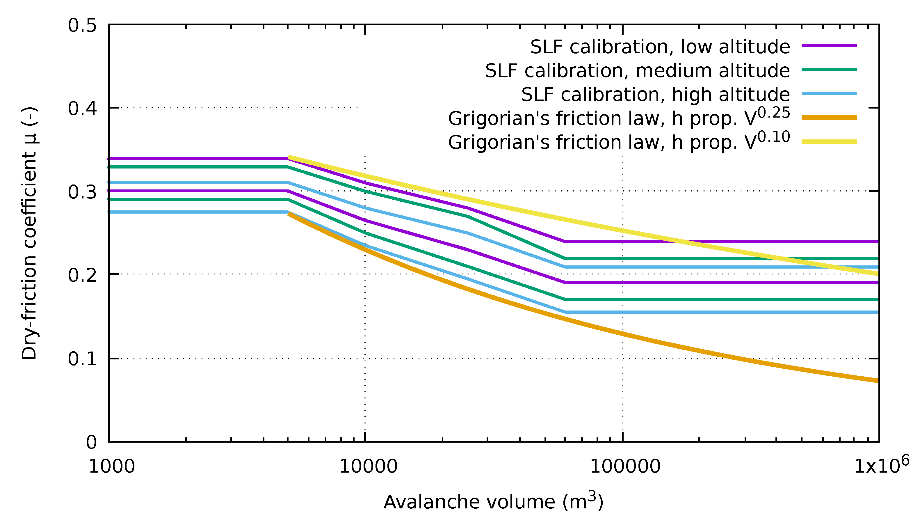
To conclude this discussion of the GFL, we ask whether it could be used to absorb the strong volume dependence in the standard calibration of the friction coefficients and k of Voellmy-type models for dry-snow avalanches. Figure 2 shows the volume dependence of according to Reference [21] for avalanches with a return period of 300 years. The different curves correspond to selected combinations of three altitude zones and four classes of terrain characteristics. Experience confirms that these values give plausible run-out distances in the majority of cases. In the range
captures the volume dependence of the calibrated values reasonably well. The GFL implies instead
is the dry-friction coefficient for . To compare the calibration of the Voellmy model to the GFL, one has to assume a (statistical) relation between the avalanche volume and the fracture depth/flow depth. Postulating , GFL matches the behavior of Equation (4) in the range (Figure 2). However, to avoid unrealistically low values for very large avalanches, h must be assumed to scale with an exponent much closer to 0 (Figure 2, yellow curve).
In which range is expected to lie? To match the calibration [21] of , should typically be reached in avalanches with a volume of 5000–10,000 m, corresponding to fracture or flow depths m. With the density in the range 200–300 , one estimates –1.5 kPa, which is encouragingly similar to the shear strength of a new-snow layer. To test the practical applicability of the GFL, one needs to compare its overall performance in a large number of avalanche cases to that of a Voellmy-type model with the standard calibration. The test cases should span a wide range of avalanche sizes, climatic conditions and terrain characteristics.
5. Some Remarks on the Grigorian–Ostroumov Erosion Model
From today’s perspective, the most relevant aspect of Reference [1] is how erosion and entrainment are modeled. The Grigorian–Ostroumov formula for the erosion rate was applied in References [27,28], but is not implemented in any code used in practice today. Below we discuss some aspects of this remarkable formula and try to assess its applicability in dynamical models of snow avalanches.
5.1. How Does the Grigorian–Ostroumov Erosion Formula Relate to Other Erosion and Entrainment Models?
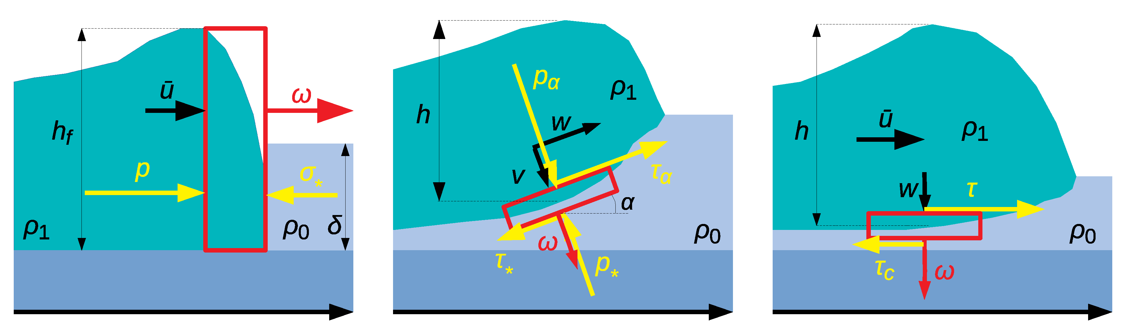
Already the first depth-averaged avalanche model by the Moscow State University group [3]—called the Eglit–Grigorian–Yakimov erosion model (EGYEM) below—described entrainment, in this case plowing entrainment at the front, formulated as a jump condition at the moving boundary of the computational domain. This entrainment mechanism can often be observed visually in slowly moving wet-snow avalanches but is absent in fast-moving dry-snow avalanches, which tend to have relatively low density at the front. Such avalanches erode the snow cover more gradually along the bottom of the flow. The Grigorian–Ostroumov erosion model (GOEM) was developed to address this situation [1]. A simpler, yet conceptually related model for basal entrainment in depth-averaged flow models that assume a uniform velocity profile and sliding at the bottom was formulated in References [29,30] and is termed tangential-jump entrainment model (TJEM) in the following. A brief comparison of the three models will help understanding the particular features of the GOEM.
These three models conceptualize the avalanche–snow cover interface as a moving non-material shock front where the eroded snow abruptly changes its velocity and usually also its density. Accordingly, jump conditions for mass and momentum (and total energy) apply at the shock. The compressive or shear strength of the snow cover enters the jump conditions for the momentum and together with the dynamical variables—flow depth, velocity, density—determines the entrainment rate uniquely; it can, in principle, be measured independent of an avalanche event, thus there are no empirical parameters that need to be fixed a posteriori. This is a fundamental difference from the vast majority of entrainment models and crucial for practical applications because no further parameter is introduced that needs to be fitted from scarce or high-uncertainty data.
The concept of the bed–flow interface being a shock applies to situations where the velocity and possibly the density change considerably in the process. One expects this to be the case if the bed material can be characterized as brittle so that erosion is a sudden process rather than a relatively slow deformation over an extended period. If the eroded material is strongly dilatant or contractive, a density shock is to be expected. These conditions are met in dense, strongly eroding gravity mass movements like snow avalanches, debris flows and pyroclastic flows that flow over beds that are granular or fracture into a granular material. They are also fulfilled in dilute flows if the erosion rate is strong, for example, in powder-snow avalanches, turbidity currents and nuées ardentes. The shock concept applies neither to slow flows over a highly plastic, cohesive bed, in which it is hard to define an interface between substrate and flow, nor to flows that only sporadically manage to erode a particle from a very strong bed, for example, a torrent flowing over bedrock.
Figure 3 shows the control volumes across which the jump conditions are evaluated. The EGYEM evaluates the jump conditions of longitudinal momentum across a vertically oriented control volume at the front end of the (expanding) computational domain. In contrast, the TJEM considers the jump in tangential momentum (determined by the longitudinal velocity and the shear stresses); it neglects the variable inclination of the erosion interface relative to the terrain surface. The GOEM accounts for the inclination of the interface relative to the terrain and evaluates the jump conditions for the momentum components normal to the interface.
5.2. The Eglit–Grigorian–Yakimov Model for Frontal Entrainment
The jump conditions in the EGYEM are essentially the same as in a hydraulic jump or bore in hydraulics. The only difference is that the pressure from the downstream side is not hydrostatic fluid pressure, but the resistance of the (solid) snow cover. A derivation of the shock velocity in terms of the depth , density , and compressive strength of the snow cover as well as the frontal flow depth , density , and near-front velocity can be found in, for example, Reference [17], the result being
The EGYEM has a number of notable features: (i) The differential mass balance equation and the equation of motion do not contain entrainment terms—all entrainment occurs at the boundary of the computational domain and manifests itself as a boundary condition. (ii) Rearranging Equation (6) as shows directly how the hydrostatic pressure exerted by the avalanche head is used partly for overcoming the resistance of the entrainable snow cover, partly for accelerating the eroded snow cover mass to the internal velocity of the avalanche. (iii) The density change from in the snow cover to in the avalanche is assumed given, but it could, in principle, be calculated from an appropriate constitutive law. (iv) The model idealizes the front as an infinitesimally thin shock, but in reality it is extended in the flow direction and the snow motion inside it is complicated, with comminution of the snow cover, compression or dilation from to and lifting of the center-of-mass from the height to . As in hydraulic jumps, some of the pressure work done by the avalanche is dissipated across the shock. The shape of the front is largely determined by the effective friction angle, implying that the control volume in reality extends over a length of the order of the flow depth.
Equation (6) assumes the hydrostatic pressure in the avalanche front to be sufficient to erode and entrain the entire erodible snow cover. In (Reference [17], Equation (5)) three alternative modifications of the model in the case of Equation (6) predicting are suggested, but no unique solution is singled out. However, the mass jump equation implies the strong constraint , that is, ; this problem deserves further study.
5.3. Main Features of the Tangential-Jump Entrainment Model
The TJEM neglects the contribution of normal pressure to the erosion process; instead, the snow cover is assumed to fracture at a critical value of the shear stress, . The difference between the shear stress exerted by the avalanche and is available for accelerating the eroded mass from rest to the avalanche velocity . Thus the tangential momentum jump condition leads to the entrainment rate
Here, if and 0 otherwise. When erosion occurs, .
Although disregarded in Reference [29], the jump conditions for mass and bed-normal momentum may also be evaluated. The mass jump condition, , implies that the flow body must have a small negative (positive) velocity w normal to the terrain if the substrate is contractive (dilatant). The jump condition for bed-normal momentum states that the eroded mass is accelerated from 0 to w by the jump in normal pressure across the interface. This effect has little practical significance, however.
At first sight, the TJEM appears to achieve closure without any adjustable parameters and is the unique consistent solution under the stated conditions. However, there is a critical hidden assumption: The bed shear stress over an eroding bed as a function of flow velocity and depth h differs in general from that over a non-erodible bed under the same flow conditions. If one considers that the interface is, in reality, a thin layer across which the eroded particles are accelerated, it is evident that the shear rate or sliding velocity at the interface between this accelerating layer and the quasi-stationary flow is less than it is at the bottom of a non-eroding flow. A simple friction law like Voellmy’s, which depends only on the depth-averaged velocity and h does not contain enough information for finding a consistent solution [30]. If one uses the standard friction law for non-erodible beds in Equation (7), one will likely overestimate the erosion rate.
5.4. Particular Features of the Grigorian–Ostroumov Erosion Model
The GOEM is based on a control volume parallel to the instantaneous interface between the avalanche and the snow cover, which is inclined by the angle relative to the terrain. Like the EGYEM, the GOEM evaluates the jump conditions for mass and the interface-normal momentum component across the control volume, which in this case read
and v are the interface-normal components of the shock propagation velocity and flow velocity, respectively. is the interface-normal stress exerted by the avalanche, the (compressive) strength of the snow cover. As in the EGYEM and TJEM, the avalanche density, , is assumed known rather than computed from a constitutive equation. Equation (9) is valid only if ; if not, . This leads to
Due to the factor , would become imaginary if . In contrast to the EGYEM and TJEM, the GOEM is thus not applicable to the fluidized and suspended parts of mixed avalanches.
Surprisingly, the Formula (10) is independent of the avalanche velocity u, and the erosion speed grows with the square root of the excess pressure, , whereas both the EGYEM and TJEM lead to an inverse dependence on the flow velocity and a linear dependence on the relevant excess stress. Technically, this comes about because v is eliminated in (9) with the help of (8). The same procedure could be applied to the EGYEM, leading to
instead of Equation (6), with . Conversely, in deriving the GOEM one can choose to substitute for in Equation (9) to obtain
showing that the erosion or entrainment speed has the same dependence on the excess stress and the interface-normal component of the flow speed in all three models.
In their review of erosion and entrainment models, Eglit and Demidov ([9], A.1.2.1) criticized the expression that Grigorian and Ostroumov use for the pressure at the interface between the avalanche and the snow cover,
is the depth-averaged velocity, h the flow depth, and the mean avalanche density, which may differ from the density at the interface, ; , where is the curvature of the path profile. There is no explanation given in Reference [1] why the second term, which resembles dynamic pressure or turbulent friction drag, should be present; neither is the origin and physical significance of the parameter C discussed. Eglit and Demidov argue that only the so-called static pressure should enter the momentum balance equation from which the jump condition is derived; the stagnation or dynamic pressure is already accounted for by the advective terms. This may explain why the entrainment speeds simulated in Reference [1] are an order of magnitude larger than observed in Nature—whenever erosion occurs in the simulations, a snowpack of 1 m is typically eroded over a distance of 5 m or less.
The simplest way to amend the GOEM would be to drop the velocity-dependent term in (10), simultaneously disposing of the empirical parameter C. This leads to smaller, more realistic entrainment rates with significantly lower values of rather than the values used in (Reference [1], Table 3). However, a more thorough analysis is warranted because the GOEM does not enforce the jump condition for the momentum tangential to the control volume, effectively treating an oblique shock as a normal shock. This work remains to be done, but a few pointers can be given here. First consider that, even though the GOEM only involves the normal stress on the interface between the avalanche and the snow cover, there is also a shear stress, . Accordingly, the maximum shear stress (inclined relative to the interface) in the new-snow layer is
where –0.35 is Poisson’s ratio for snow [31] and is in the range , typically –0.8. With the typical range , the two terms in (14) are of similar magnitude, but there may be a significant velocity dependence in . The threshold condition for erosion in (10) thus should be , with from Equation (14) and the shear strength of the snow cover. Next, examine and ; they refer to the interface, which is inclined at the angle to the terrain, relative to which the flow model is formulated. The tensor transformation laws lead to
The hydrostatic pressure is assumed isotropic. If , the bed shear stress tangential to the terrain, is calculated from the Voellmy friction law, Equations (13) and (15) behave qualitatively similar.
The next task is to relate to the shear strength so that the shock propagation velocity can be computed. The GOEM disregards the shear stresses at the interface so that Equation (14) simplifies to and one obtains in terms of the shear strength of the snow cover. However, the problem is more involved with shear stresses because there is no justification for assuming that the ratio between and remains unchanged across the shock. At this point, one needs to use the constraint from the jump condition for the interface-parallel momentum component:
If one assumes a uniform velocity profile and neglects the small component of parallel to the terrain, and , implying that the jump in the shear stress accelerates the eroded mass to the mean avalanche speed as in the TJEM. (not to be confused with in Grigorian’s modified friction law, see Section 4) indicates the critical shear stress along the interface; it is related to and by
The shock speed has to be the same, whether calculated from Equation (12) or (19), requiring
and are given by Equations (15) and (16) and related to the maximum shear stress by (14). This leads to a quadratic equation with the solution
To find the approximate conditions for the existence of a physical solution, assume the erosion angle to be small—measurements at Vallée de la Sionne point towards typical values of 0.01 or less. Then, and . Furthermore, the ratio is typically in the range 0.3–1. A physical solution to Equation (20) thus only exists if , , , and . Hence, a rough estimate for the admissible range of the hydrostatic pressure is
The lower limit of is typically (0.9–1.5) , the upper limit (1.2–1.7) .
If falls below the lower limit, entrainment ceases. What happens if exceeds the upper limit? On the one hand, the conditions for erosion, that is, the propagation of the shock, are still fulfilled and obtained from Equation (12) increases with . On the other hand, is too small to satisfy Equation (19). This means that the eroded mass cannot be accelerated to the full avalanche speed at once and forms a bottom layer that is dragged along by the main flow above.
5.5. Can the Grigorian–Ostroumov Erosion Formula Be Used in Practice?
The importance of modeling entrainment has been acknowledged among avalanche dynamics researchers for half a century, but it will probably still take years until flow models with entrainment (and deposition) become a standard in avalanche hazard mapping procedures. There are both a fundamental modeling problem and a number of practical issues to be overcome.
On the practical side, the following challenges persist: (i) Data suitable for testing entrainment models is still scarce. (ii) Entrainment models can be validated only in conjunction with a specific avalanche rheology or bed friction law. (iii) Many authors argue that entrainment models just add to the list of poorly constrained initial conditions and friction parameters (see, e.g., Reference [22]). First, published data [27,32] already allows for at least qualitative validation. The situation can be further improved by pooling observations and data from different sites to create a sound basis for quantitatively validating dynamical models. The second problem can be approached by implementing the EGYEM, GOEM and TJEM in flow models based on different friction laws or rheologies and comparing their performance with and without entrainment for selected test cases. Thirdly, a practical method needs to be developed for prescribing the erodible snow depth and the shear strength as functions of the return period, regional precipitation data, winter temperature, slope orientation, and the dominant wind directions. This task appears feasible where distributed data of temperature, snow depth and precipitation are available; however, additional measurements of snow shear strength at different altitudes and under different topographical conditions might also be required.
The first theoretical problem is to understand how the snow-strength parameter in the GOEM, the limit shear strength in the GFL, in the EGYEM and in the TJEM are related to each other and to measurable properties of the snow cover. At this point, only a tentative answer can be offered. First, note that all four process models for friction or erosion originally refer to the top layer of the substrate (the new-snow layer in the case of snow avalanches). However, a weak layer underneath the top layer or poor bonding between the layers will greatly influence the behavior of the system; with regard to the erosion models, see the discussion below. In the GFL and TJEM, shear stresses are transmitted across a competent top layer to the weak layer, which will fail before the top layer. Thus, the shear strength of the weakest layer is decisive. In the original GOEM, the propagation of the primary shock front is determined by the strength of the top layer, but the normal stress is transmitted across the top layer and may induce failure of a weak layer or interface underneath. Describing this situation is, however, beyond the scope of the GOEM. Perhaps surprisingly, the weak-layer shear strength does not contribute to the momentum jump condition in the EGYEM if the shock is infinitesimally thin. This implies that the strength of the top layer is the decisive parameter in the EGYEM whereas the weak layer determines the erosion depth. In a refined version of the EGYEM with a finite-width transition zone, the weak-layer strength will contribute to some degree.
A second point to note is that the parameters of all four process models are failure criteria for a solid under given normal and shear stresses. All models implicitly assume that there are confining lateral stresses (only in the spanwise direction for the EGYEM). This implies that both the normal and the shear stress have to be taken into account to determine the maximum shear stress, as shown in Equation (14). The failure criterion is exceeding the shear strength of the snow cover. The GOEM, TJEM and GFL neglect one of the two contributions to , but this can easily be improved. The shear strength of snow can, in principle, be determined as half the difference between the major and minor normal stress at failure in a triaxial compression test—a standard procedure in soil mechanics. However, with snow these tests have to be conducted at high compression rates to enter the brittle-failure regime.
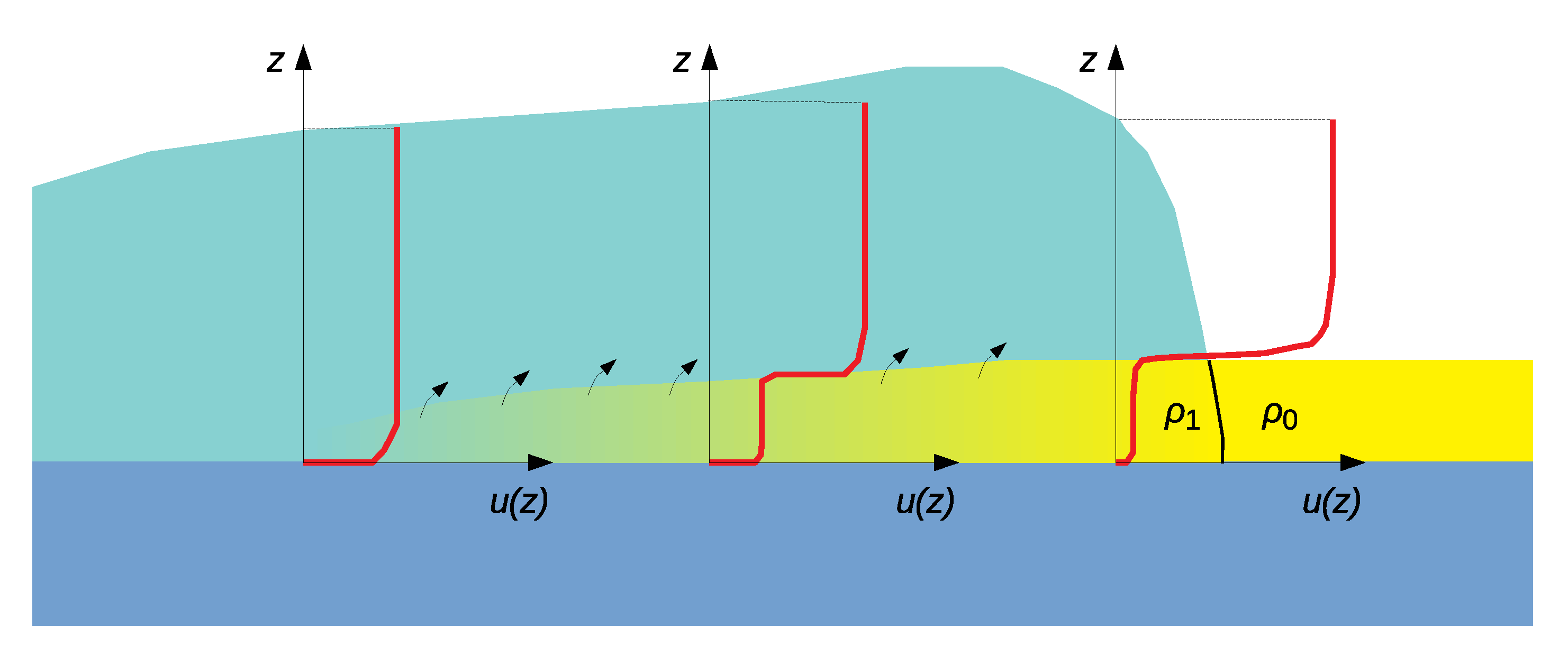
The second theoretical question in entrainment modeling concerns the layered structure of natural snowpacks: Profiling-radar measurements at the test site Vallée de la Sionne in 1999 gave evidence for continuous, scouring-type erosion and entrainment ([33], Figure 3) as described by the GOEM or TJEM. However, later measurements at the same locations frequently show step-wise (“ripping” [34]) erosion [27,28] where the erosion front at the radar location quasi-instantaneously jumps, presumably either because the layer is weak or because a weak layer underneath fails. In general, one has to expect that both erosion modes coexist in the same event. We conjecture that scouring occurs when the new-snow shear strength increases with depth and the layer bonds well to the underlying snowpack. With step-wise erosion, the eroded slab is too massive to be entrained immediately. It is compressed, comminuted and gradually accelerated while the erosion front advances with the avalanche front.
A simple approach to this problem is to disregard the weak layer and to use a model for scouring erosion, hoping that the effects of delayed entrainment are small on the scale of the entire flow. Alternatively, one may envisage an extended model that treats the new-snow layer as dynamical. Where the shear stress at the interface to the old snow exceeds the weak-layer shear strength , fracture is assumed and is replaced by a suitable friction law. The slab is accelerated by the difference in the shear stresses from the avalanche and the substrate and by the longitudinal pressure gradient. The mass-exchange term between the two layers should describe instantaneous entrainment of a slab segment when the relative velocity difference is nearly zero. The model should also account for possible scouring entrainment from the moving slab into the avalanche. Transforming this concept (Figure 4) into a consistent set of equations and a working model is left for future work.
The time appears right for a new attempt to solve the problem of entrainment and deposition—Sovilla et al. [35] found inclusion of entrainment to improve the modeling results when compared to observations and to substantially reduce the unphysical scatter of friction parameter values needed to reproduce the observed run-out distances. Recently, Rauter and Köhler [36] demonstrated that two rather dissimilar avalanches released in the same path on the same day could be modeled with the same parameter set, provided that the avalanche model accounts for both entrainment and deposition. The GOEM (with the modifications discussed above and preferably an extension for dynamically calculating the avalanche density) provides a physically consistent description of continuous, scouring erosion of a homogeneous snowpack without empirical parameters. Being one of the few serious contenders in this field, it clearly deserves further study.
6. Do Avalanches Behave Non-Monotonically in the Friction Coefficients?
Probably the most surprising finding in Reference [1] is the non-monotonic behavior with regard to variations of the dry-friction parameter under otherwise identical conditions: The avalanche “ignited” only in a limited range of , both with larger or smaller friction coefficients entrainment soon ceased and the flow stopped. Such behavior was observed only in the complete model and only if both GFL and the GOEM were activated [18]. If such behavior were to generally occur in models with non-smooth friction law and a threshold for entrainment, the practical usefulness of advanced, complex models would be put in question. One way to investigate this problem is to reimplement the “complete” model as a numerical code to confirm that the observed non-monotonous behavior is not caused by numerical artifacts and to explore the phase diagram of the model.
Grigorian and Ostroumov did not observe non-monotonic behavior in the “simplified” models, but those models do not include entrainment, which seems to be an essential prerequisite for this phenomenon to occur. It may therefore be instructive to study the “simplified” model enhanced by an entrainment term derived from the GOEM because it has only two degrees of freedom—the maximum of the instantaneous flow depth, H, and the front velocity U—in contrast to the infinite number of degrees of freedom contained in the fields and of the “complete” model. One can thus study such an “enhanced simplified” model with the techniques developed in the mathematical theory of dynamical systems. In principle, this can be done for any given path profile described by , but in practice one will select a few elementary types like an inclined plane or the hockeystick profile with slope angle .
Such a study remains yet to be done, but we briefly derive the set of equations here. The mass balance, initially expressed as an integral over space and time,
transforms into a spatial evolution equation for the longitudinal section area with if one uses the front position as the independent variable instead of the time and sets :
The equation of motion reads
The appearance of an integral in (24) but not in (25) is a direct consequence of the assumptions that (i) the shape of the longitudinal section of the avalanche remains self-similar and (ii) only the front is relevant for the dynamics of the flow. To evaluate Equation (24), some further simplifying assumptions are required. Grigorian and Ostroumov mention that the shape of the avalanche is well described by the parabola
which leads to the value for the shape parameter, close to the recommended value 0.36. If there were no entrainment, self-similarity of the shape through time would imply
In the presence of entrainment (which diminishes with distance from the front), the velocity must be smaller than the value given by Equation (27) so that part of the eroded snow is transported towards the tail to maintain the parabolic shape. However, for the purpose of investigating the qualitative properties of this dynamical system, it seems justifiable to use Equation (27) as an approximation. The integral over the erosion rate can then be evaluated in terms of H and U, the resulting expression depending on the one choice for the pressure , as discussed in Section 5.4.
The two Equations (24) and (25) determine the trajectories of the system in the phase space . Of particular interest are its fixed points, that is, pairs of values for which , and critical lines with . Fixed points —corresponding to avalanches that stop—can exist only if over a suitable interval in . In contrast to the classic examples of dynamical systems found in textbooks, the Grigorian–Ostroumov model on a hockeystick profile with slope angles has a continuum of such fixed points, with their basins of attraction degenerated to a single line.
In Reference [37], a rather general asymptotic solution to a simplified model for an entraining flow on an infinite inclined plane was found; it corresponds to a critical line tending to a straight line parallel to . A characteristic property of that model is that the bed shear stress is limited to the shear strength of the snow (the TJEM is a limiting case with the depth of the shear layer shrunk to 0). It remains to be seen whether such a solution also exists for the Grigorian–Ostroumov model.
Once the structure of the phase space with its fixed points, critical lines and basins of attraction is determined for given values of , , k, and , one may proceed to study the dependence of this structure on , with the other three parameters held fixed. Figure 5 visualizes the dependence of the phase-space structure for different values of in a strongly simplified way. The non-monotonicity found in Reference [1] would manifest itself in the way that some starting point in the phase space lies within the basin of attraction of some fixed point for and , but belongs to the basin of attraction of another fixed point or tends towards a critical line with if .
Almost half a century after the main work by Grigorian and Ostroumov summarized in Reference [1] and close to a quarter century since the writing of that paper, our insight into the flow behavior of snow avalanches has been dramatically deepened through new experiments, and a large number of new numerical models have been developed and are being applied in practical work. Yet, the span of topics discussed in the present Comments paper, the open questions raised by the Grigorian–Ostroumov model and the new avenues for research that a fresh reading of their paper suggests are proof enough that this work can inspire the work of today’s generation of avalanche researchers. The same holds for early and more recent work summarized in the review paper by Eglit et al. [17], which extends the scope of Reference [1].
Funding
The writing of this paper was in part supported by NGI’s Strategic Projects SP 4—Snow Avalanche Research and SP 11 MERRIC—Multi-scale Erosion Risk under Climate Change. The latter is jointly funded by the Research Council of Norway and NGI, the former by the Norwegian Petroleum and Energy Department through a grant administrated by the Norwegian Directorate of Water Resources and Energy.
Acknowledgments
D.I. thanks A. V. Ostroumov and M. E. Eglit for their most valuable help with a number of technical points concerning the Eglit–Grigorian–Yakimov and Grigorian–Ostroumov erosion models as well as for supplementing aspects of the history of Reference [1]. Insightful remarks from an anonymous reviewer improved the manuscript.
Conflicts of Interest
The author declares no conflict of interest. The funders had no role in the writing of the manuscript, or in the decision to publish it.
References
- Grigorian, S.S.; Ostroumov, A.V. On a continuum model for avalanche flow and its simplified variants. Geosciences 2020, 10, 35. [Google Scholar] [CrossRef] [Green Version]
- Voellmy, A. Über die Zerstörungskraft von Lawinen. Schweiz. Bauztg. 1955, 73, 159–165, 212–217, 246–249, 280–285. [Google Scholar]
- Briukhanov, A.V.; Grigorian, S.S.; Miagkov, S.M.; Plam, M.Y.; Shurova, I.Y.; Eglit, M.E.; Yakimov, Y.L. On some new approaches to the dynamics of snow avalanches. In Physics of Snow and Ice, Proc. Intl. Conf. Low Temperature Science, Sapporo, Japan, 1966; Ôura, H., Ed.; Institute of Low Temperature Science, Hokkaido University: Sapporo, Japan, 1967; Volume I, Part 2; pp. 1223–1241. [Google Scholar]
- Savage, S.B.; Hutter, K. The motion of a finite mass of granular material down a rough incline. J. Fluid Mech. 1989, 199, 177–215. [Google Scholar] [CrossRef]
- Eglit, M.E. Teoreticheskie podkhody k raschetu dvizheniia snezhnyk lavin. (Theoretical approaches to avalanche dynamics). Itogi Nauki. Gidrologiia Sushi. Gliatsiologiia 1967, 69–97. (In Russian) English translation in: Soviet Avalanche Research—Avalanche Bibliography Update: 1977–1983. Glaciological Data Report GD–16, pages 63–116. World Data Center A for Glaciology [Snow and Ice], 1984 [Google Scholar]
- Bakhvalov, N.S.; Eglit, M.E. Issledovanie reshenii upravlenii dvizheniia snezhnykh lavin (Investigations of the solutions to snow avalanche movement equations). Akad. Nauk SSSR Inst. Geogr. Mat. Gliatsol. Issledov. Khr. Obsuzhdeniia 1969, 15, 31–38. (In Russian) Translated in: Glaciological Data, Soviet Avalanche Research—Avalanche Bibliography Update: 1977–1983, World Data Center A for Glaciology, Boulder, CO, USA, Report GD-16, 1984 [Google Scholar]
- Eglit, E.M. Some mathematical models of snow avalanches. In Advances in the Mechanics and the Flow of Granular Materials, 1st ed.; Shahinpoor, M., Ed.; Trans Tech Publications: Clausthal-Zellerfeld, Germany, 1983; Volume II, pp. 577–588. [Google Scholar]
- Eglit, M.E. Mathematical and physical modelling of powder-snow avalanches in Russia. Ann. Glaciol. 1998, 26, 281–284. [Google Scholar] [CrossRef]
- Eglit, M.E.; Demidov, K.S. Mathematical modeling of snow entrainment in avalanche motion. Cold Reg. Sci. Technol. 2005, 43, 10–23. [Google Scholar] [CrossRef]
- Kulibaba, V.S.; Eglit, M.E. Numerical modeling of an avalanche impact against an obstacle with account of snow compressibility. Ann. Glaciol. 2008, 49, 27–32. [Google Scholar] [CrossRef] [Green Version]
- Eglit, M.E.; Yakubenko, A.E. Numerical modeling of slope flows entraining bottom material. Cold Reg. Sci. Technol. 2014, 108, 139–148. [Google Scholar] [CrossRef]
- Grigorian, S.S. Mechanics of snow avalanches. In Snow Mechanics Symposium Mécanique de la Neige— Proceedings of the Grindelwald Symposium, April 1974; LaChapelle, E.R., Kuroiwa, D., Salm, B., Eds.; International Association of Hydrological Sciences: Wallingford, UK, 1975; pp. 355–368. [Google Scholar]
- Grigoryan, S.S.; Urumbayev, N.A. On the nature of an avalanche air wave. Nauchnye trudy Instituta Mekhaniki Moskovskogo Gosudarstvennogo Universiteta [Scientific Works of the Institute of Mechanics of Moscow State University] 1975, 42, 74–82. (In Russian) English translation in: 34 Selected Papers on Main Ideas of the Soviet Glaciology, 1940s–1980s. Kotlyakov, V.M., Ed.; Glaciological Association of Russia: Moscow, Russia, 1997; pp. 289–296. [Google Scholar]
- Grigoryan, S.S. A new law of friction and mechanism for large-scale avalanches and landslides. Sov. Phys. Dokl. 1979, 24, 110–111. [Google Scholar]
- Sadovnichii, V.A.; Nigmatulin, R.I. Samvel Samvelovich Grigoryan (On his Eightieth Birthday). J. Appl. Math. Mech. 2010, 74, 255–266. [Google Scholar] [CrossRef]
- Available online: https://cordis.europa.eu/event/rcn/1575/en (accessed on 31 May 2019).
- Eglit, M.E.; Yakubenko, A.; Zayko, J. A review of Russian snow avalanche models—From analytical solutions to novel 3D models. Geosciences 2020, 10, 77. [Google Scholar] [CrossRef] [Green Version]
- Ostroumov, A.V.; (Institute of Mechanics, Lomonossov State University, Moscow, Russia). Personal communication, to D. Issler. September 2019.
- Kulikovskiy, A.G.; Sveshnikova, Y.I. Model’dlya rasheta dvizheniya pylevoy snezhnoy laviny (A model for calculating the motion of a powder-snow avalanche). Mater. Glyatsiol. Issled. 1977, 31, 74–80. (In Russian) [Google Scholar]
- Dade, W.B.; Huppert, H.E. A box model for non-entraining, suspension-driven gravity surges on horizontal surfaces. Sedimentology 1995, 42, 453–471. [Google Scholar] [CrossRef]
- Bartelt, P.; Bühler, Y.; Christen, M.; Deubelbeiss, Y.; Salz, M.; Schneider, M.; Schumacher, L. RAMMS::AVALANCHE User Manual; WSL Institute for Snow and Avalanche Research SLF: Davos Dorf, Switzerland, 2017. [Google Scholar]
- Salm, B. A short and personal history of snow avalanche dynamics. Cold Reg. Sci. Technol. 2004, 39, 83–92. [Google Scholar] [CrossRef]
- Gauer, P. Comparison of avalanche front velocity measurements and implications for avalanche models. Cold Reg. Sci. Technol. 2014, 97, 132–150. [Google Scholar] [CrossRef]
- McClung, D.M.; Gauer, P. Maximum frontal speeds, alpha angles and deposit volumes of flowing snow avalanches. Cold Reg. Sci. Technol. 2018, 153, 78–85. [Google Scholar] [CrossRef]
- Bozhinskiy, A.N.; Losev, K.S. The Fundamentals of Avalanche Science; Institut für Schnee- und Lawinenforschung: Davos, Switzerland, 1998. [Google Scholar]
- De Blasio, F.V.; Medici, L. Microscopic model of rock melting beneath landslides calibrated on the mineralogical analysis of the Köfels frictionite. Landslides 2017, 14, 337–350. [Google Scholar] [CrossRef]
- Sovilla, B. Field Experiments and Numerical Modelling of Mass Entrainment and Deposition Processes in Snow Avalanches. Ph.D. Thesis, ETH Zürich, Zürich, Switzerland, 2004. [CrossRef]
- Sovilla, B.; Burlando, P.; Bartelt, P. Field experiments and numerical modeling of mass entrainment in snow avalanches. J. Geophys. Res. 2006, 111, F03007. [Google Scholar] [CrossRef]
- Issler, D.; Jóhannesson, T. Dynamically Consistent Entrainment and Deposition Rates in Depth-Averaged Gravity Mass Flow Models; NGI Technical Note 20110112-01-TN; Norwegian Geotechnical Institute: Oslo, Norway, 2011. [Google Scholar] [CrossRef]
- Issler, D. Dynamically consistent entrainment laws for depth-averaged avalanche models. J. Fluid Mech. 2014, 759, 701–738. [Google Scholar] [CrossRef] [Green Version]
- Shapiro, L.H.; Johnson, J.B.; Sturm, M.; Blaisdell, G.H. Snow Mechanics—Review of the State of Knowledge and Applications; CRREL Report 97-3; US Army Corps of Engineers, Cold Regions Research and Engineering Laboratory: Hanover, NH, USA, 1997.
- Sovilla, B.; Sommavilla, F.; Tomaselli, A. Measurements of mass balance in dense snow avalanche events. Ann. Glaciol. 2001, 32, 230–236. [Google Scholar] [CrossRef] [Green Version]
- Issler, D. Experimental information on the dynamics of dry-snow avalanches. In Dynamic Response of Granular and Porous Materials under Large and Catastrophic Deformations; Lecture Notes in Applied and Computational Mechanics; Hutter, K., Kirchner, N., Eds.; Springer: Berlin, Germany, 2003; Volume 11, pp. 109–160. [Google Scholar] [CrossRef]
- Gauer, P.; Issler, D. Possible erosion mechanisms in snow avalanches. Ann. Glaciol. 2004, 38, 384–392. [Google Scholar] [CrossRef] [Green Version]
- Sovilla, B.; Margreth, S.; Bartelt, P. On snow entrainment in avalanche dynamics calculations. Cold Reg. Sci. Technol. 2007, 47, 69–79. [Google Scholar] [CrossRef]
- Rauter, M.; Köhler, A. Constraints on Entrainment and Deposition Models in Avalanche Simulations from High-Resolution Radar Data. Geosciences 2020, 10, 9. [Google Scholar] [CrossRef] [Green Version]
- Issler, D.; Pastor Pérez, M. Interplay of entrainment and rheology in snow avalanches: A numerical study. Ann. Glaciol. 2011, 52, 143–147. [Google Scholar] [CrossRef] [Green Version]
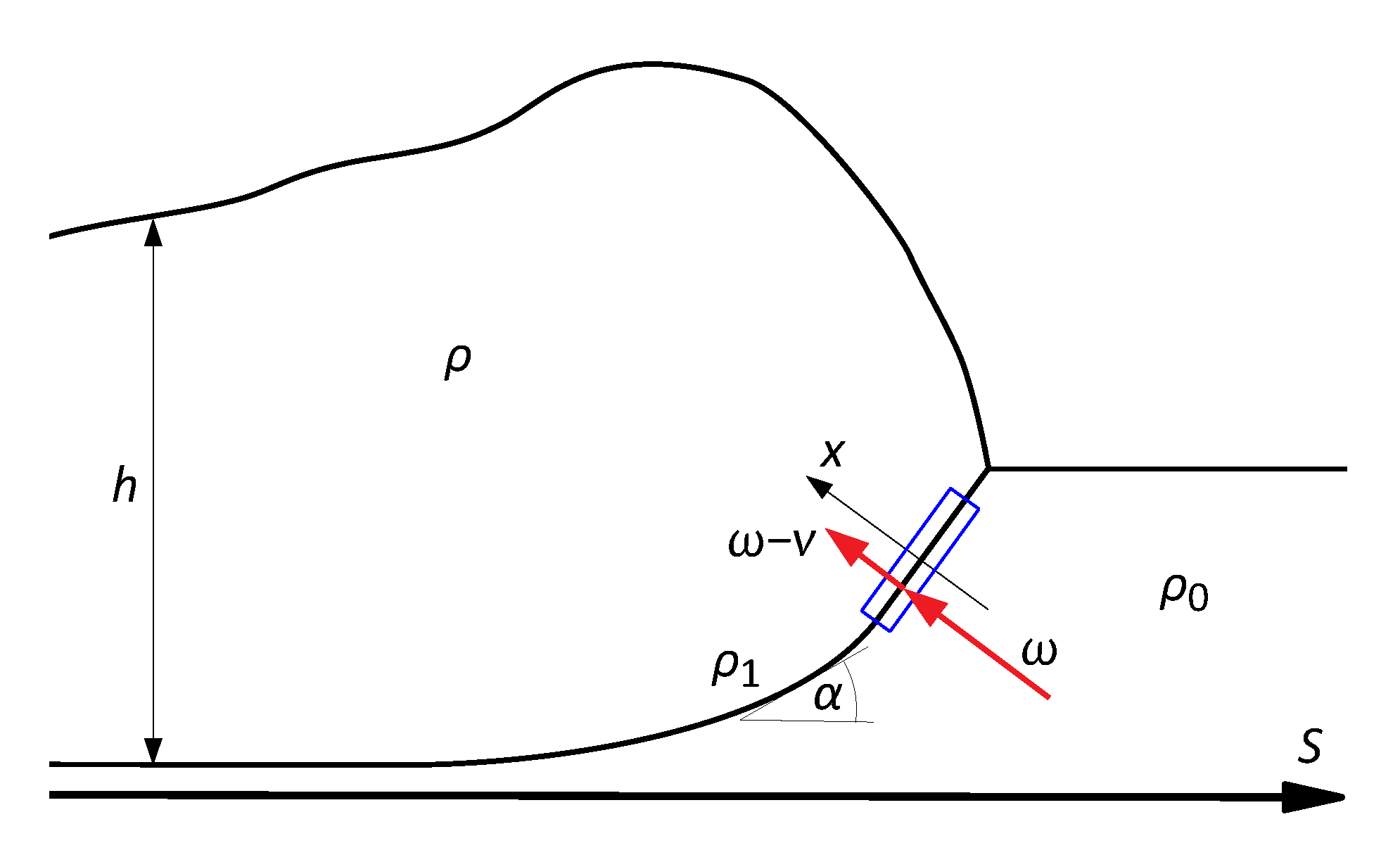
Figure 1.
Schematic representation of the integration volume (blue box) for the mass and momentum jump conditions across the interface between snowcover (density ) and avalanche (density ). The normal velocity components on both sides of the interface (red arrows) refer to the coordinate system moving with the front.

Figure 2.
Volume dependence of dry-friction coefficient in the recommended calibration for the flow model RAMMS::AVALANCHE for different altitude zones and two types of terrain characteristics. With an assumed scaling relation , the Grigorian’s friction law (GFL) captures that behavior well up to (brown curve). To avoid large discrepancies for large volumes, the scaling exponent of h needs to be reduced to about 0.1 (yellow curve).

Figure 3.
Control volumes used in the derivation of the Eglit–Grigorian (EGYEM, left), Grigorian–Ostroumov (GOEM, middle), and tangential-jump (TJEM, right) entrainment models. Note that the EGYEM and GOEM evaluate the jump equations for the velocity and momentum components normal to the “long” side of the control volume while the TJEM considers tangential velocity and shear stresses.

Figure 4.
Schematic representation of the entrainment process for entire slabs. At the avalanche front, the new-snow layer (yellow, density ) is compressed to density , but only partially accelerated, as shown by the rightmost velocity profile. Friction from the overriding avalanche body (turquoise) reduces the velocity deficit of the slab (represented by color changing from yellow to turquoise) until it becomes a part of the main body. During the process, scouring entrainment may also occur (small arrows).

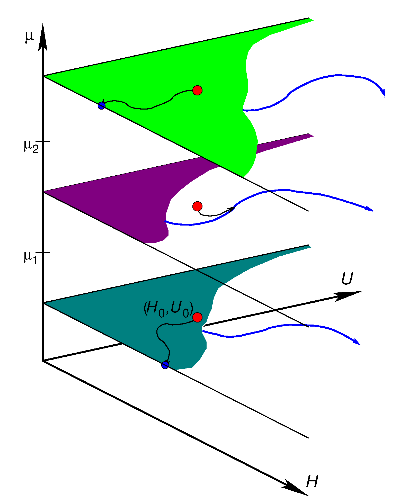
Figure 5.
Strongly simplified representation of a hypothetical structure of the phase space of the “enhanced simplified” Grigorian–Ostroumov model. Three copies of the phase-space plane, representing different values of the friction coefficient , are shown; the parameters k, and are held fixed. The red dots mark an (arbitrarily chosen) initial condition . The avalanche evolves either to a final rest state indicated by the blue points on the axis (if or ) or towards and along a critical line (in blue) that approaches either a fixed point corresponding to a moving steady state or to a state where the avalanche grows and/or accelerates indefinitely. The colored areas indicate the basin of attraction of the fixed points on the axis .

© 2020 by the author. Licensee MDPI, Basel, Switzerland. This article is an open access article distributed under the terms and conditions of the Creative Commons Attribution (CC BY) license (http://creativecommons.org/licenses/by/4.0/).
Share and Cite
MDPI and ACS Style
Issler, D. Comments on “On a Continuum Model for Avalanche Flow and Its Simplified Variants” by S. S. Grigorian and A. V. Ostroumov. Geosciences 2020, 10, 96. https://doi.org/10.3390/geosciences10030096
AMA Style
Issler D. Comments on “On a Continuum Model for Avalanche Flow and Its Simplified Variants” by S. S. Grigorian and A. V. Ostroumov. Geosciences. 2020; 10(3):96. https://doi.org/10.3390/geosciences10030096
Chicago/Turabian StyleIssler, Dieter. 2020. "Comments on “On a Continuum Model for Avalanche Flow and Its Simplified Variants” by S. S. Grigorian and A. V. Ostroumov" Geosciences 10, no. 3: 96. https://doi.org/10.3390/geosciences10030096
Note that from the first issue of 2016, this journal uses article numbers instead of page numbers. See further details here.