Application of a Model-Based Controller for Improving Internal Combustion Engines Fuel Economy


Department of Mechanical, Energy and Management Engineering, University of Calabria, Ponte Bucci, Cubo 46C, 87036 Rende, Italy
*
Author to whom correspondence should be addressed.
Energies 2020, 13(5), 1148; https://doi.org/10.3390/en13051148
Submission received: 23 January 2020
/
Revised: 17 February 2020
/
Accepted: 20 February 2020
/
Published: 3 March 2020
(This article belongs to the Special Issue Advances in Spark-Ignition Engines)
Abstract
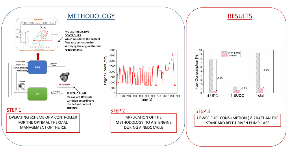
:Improvements in internal combustion engine efficiency can be achieved with proper thermal management. In this work, a simulation tool for the preliminary analysis of the engine cooling control is developed and a model-based controller, which enforces the coolant flow rate by means of an electrically driven pump is presented. The controller optimizes the coolant flow rate under each engine operating condition to guarantee that the engine temperatures and the coolant boiling levels are kept inside prescribed constraints, which guarantees efficient and safe engine operation. The methodology is validated at the experimental test rig. Several control strategies are analyzed during a standard homologation cycle and a comparison of the proposed methodology and the adoption of the standard belt-driven pump is provided. The results show that, according to the control strategy requirements, a fuel consumption reduction of up to about 8% with respect to the traditional cooling system can be achieved over a whole driving cycle. This proves that the proposed methodology is a useful tool for appropriately cooling the engine under the whole range of possible operating conditions.

1. Introduction
Steadily increasing challenges for climate change are leading to the development of new technologies for sustainable mobility, which include powertrain electrification like hybrids, plug-in hybrids, and fully electric vehicles. These solutions provide a very interesting opportunity in terms of fuel-saving and air quality, especially in very congested areas; however, they have the drawback of being expensive and some environmental issues seen from a life-cycle assessment (LCA) point of view are still unresolved [1]. In this context, internal combustion engines, and in particular spark ignition (SI) engines, still offer significant developmental margins to meet future requirements, both in terms of CO2 emissions reduction within the limits prescribed by the regulatory agencies [2,3] and in terms of engine performance and will presumably be widespread in the automotive industry for the next few decades [4].
Several technical solutions have been developed to optimize SI engines in terms of fuel consumption, performance, and emissions. Gasoline engines “downsizing” and supercharging boosting [5], innovative intake strategies [6,7,8], cooled external exhaust gas recirculation [9], and innovative after-treatment technologies [10,11] have been shown to improve the efficiency of spark-ignited gasoline engines. A further contribution to fuel consumption reduction is given by the adoption of an optimized engine thermal management [12,13]. In fact, with optimized thermal management, a contribution of about 3% over the total CO2 decrease was estimated [5] and, if compared to different technological options, it is the most cost-effective by accounting for about 200 Euro/(km/L saved) [14].
The primary requirement of optimized thermal management is the reduction of the warm-up time, which, by speeding-up lubricant heating, reduces frictional losses [13,14,15] and improves engine efficiency as a direct consequence. Lower coolant flow rates than the ones delivered by the traditional engine cooling system are, therefore, needed in this case. On the contrary, higher coolant flow rates than the ones commonly used under low-speed, high-load conditions, can be effective in mitigating knock and, therefore, diminishing the use of more fuel-consuming strategies like spark retard and mixture enrichment [16]. Unfortunately, the regulation capabilities of a standard engine cooling system are restricted by the adoption of a crank-shaft driven pump and a wax thermostat valve. These devices cause engine overcooling for about 95% of its operating time [17], during which the single-phase forced convection takes place. The possibility of optimizing the cooling system relies, therefore, on the removal of the standard crankshaft-driven pump and the inclusion of electrically driven pumps and of advanced electronic actuators, associated with proper control strategies. Solutions, which include an electrically driven pump, whose control is based on empirical methods can be found in [18,19], where improvement in specific fuel consumption of up to 2% is achieved. The adoption of electrically driven pumps and actuators presents a further advantage: the possibility of moving towards nucleate boiling flow regimes and to achieve a precision cooling strategy, which can provide a reduction in warm-up time of about 18% and a remarkable reduction of the power supplied to the coolant pump (up to 1.85 kW) [20]. To this aim, more sophisticated control approaches than the empirical ones are needed for keeping the boiling regime under control.
A control method, which has gained attention in recent years, is model predictive control (MPC), which permits the control of multi-input multi-output (MIMO) systems with constraints in an optimized way [21] and has found wide application in many slow-dynamic areas of engine control [22,23]. MPC was primarily implemented on compression-ignition (CI) engines [24,25,26] and recent attempts on spark-ignited (SI) engines [27,28,29] have also been proposed. The working principle of the MPC is based on the definition of a quadratic cost function, which integrates the deviation of an engine parameter from its desired values over a period of time, which is the prediction horizon; the cost function is minimized by manipulating the actuator set-points; in such a way, the optimal control actions are determined. In particular, the MPC algorithm requires the use of an engine model, which determines the current state of the engine from the sensors signals; the model is linearized about the current states and is then used to determine new actuator set-points that meet the cost function requirements within prescribed constraints. Linearization is carried out off-line for a variety of operating points and the results of the optimization problem are stored in the onboard controller.
A systematic control approach for the optimal thermal management of the coolant flow rate in an SI engine, based on MPC, was proposed by Pizzonia et al. [30]. The controller is based on the development of an engine thermal model, which predicts the heat transfer regime occurring between the engine walls and the coolant for a given engine operating condition. The model also predicts the occurrence of nucleate boiling and defines an index, namely the NB_Index, which operates as a virtual sensor for the detection of the boiling intensity. The control actuator is an electric pump, which gives the possibility of operating with reduced coolant flow rates when compared to the ones delivered by the belt-driven pump. The controller can also operate higher coolant flow rates under low-speed, high-load conditions and can keep the pump running after engine switch-off to avoid after-boiling [31,32,33].
In this work, a simulation tool for the proposed controller is developed with the aim to preliminarily evaluate different control strategies and give an estimation of the controller’s effectiveness in terms of constraint requirements and engine efficiency. The proposed engine simulator is validated at the experimental test rig during a standard homologation cycle. Then, a variety of controllers are proposed and the benefits in terms of fuel consumption reduction, when compared to the crankshaft-driven pump, are quantified.
The model developed for the controller design and the controller working principle are summarized in Section 2. A simulation algorithm, which predicts the controller behavior, is validated in Section 3. Different control strategies are developed and simulated during a New European Driving Cycle (NEDC) homologation cycle and the results in terms of fuel consumption reduction and CO2 emissions are presented in Section 4. Several engine operating conditions different from the NEDC cycle are analyzed in Section 5. Finally, the achieved results are discussed in Section 6.
2. Materials and Methods
The proposed approach is based on the development of a controller, which is able to optimize the coolant flow rate in the presence of nucleate boiling. For this purpose, a lumped-parameters model for the thermal exchange between the coolant and the engine walls is developed. The model predicts the occurrence of nucleate boiling by defining a metric for nucleate boiling detection. An extensive description of the model and controller is included in [30,34]; however, both the model and the controller are briefly described in the following subsections for the sake of clarity.
In the present work, the operating scheme of the controller is implemented numerically, with the aim to preliminarily simulate its behavior under various engine operating conditions, to predict the effects of the control strategy on fuel consumption and eventually to improve the controller design. The controller is also implemented at the experimental test rig and is tested under real engine operation.
2.1. Engine Thermal Model
A zero-dimensional approach is adopted for modeling the heat transfer between the engine walls and the coolant; the model dynamically predicts the occurrence of nucleate boiling [34]. The spatial-averaged wall and coolant temperatures, and are obtained from the following energy conservation equations:
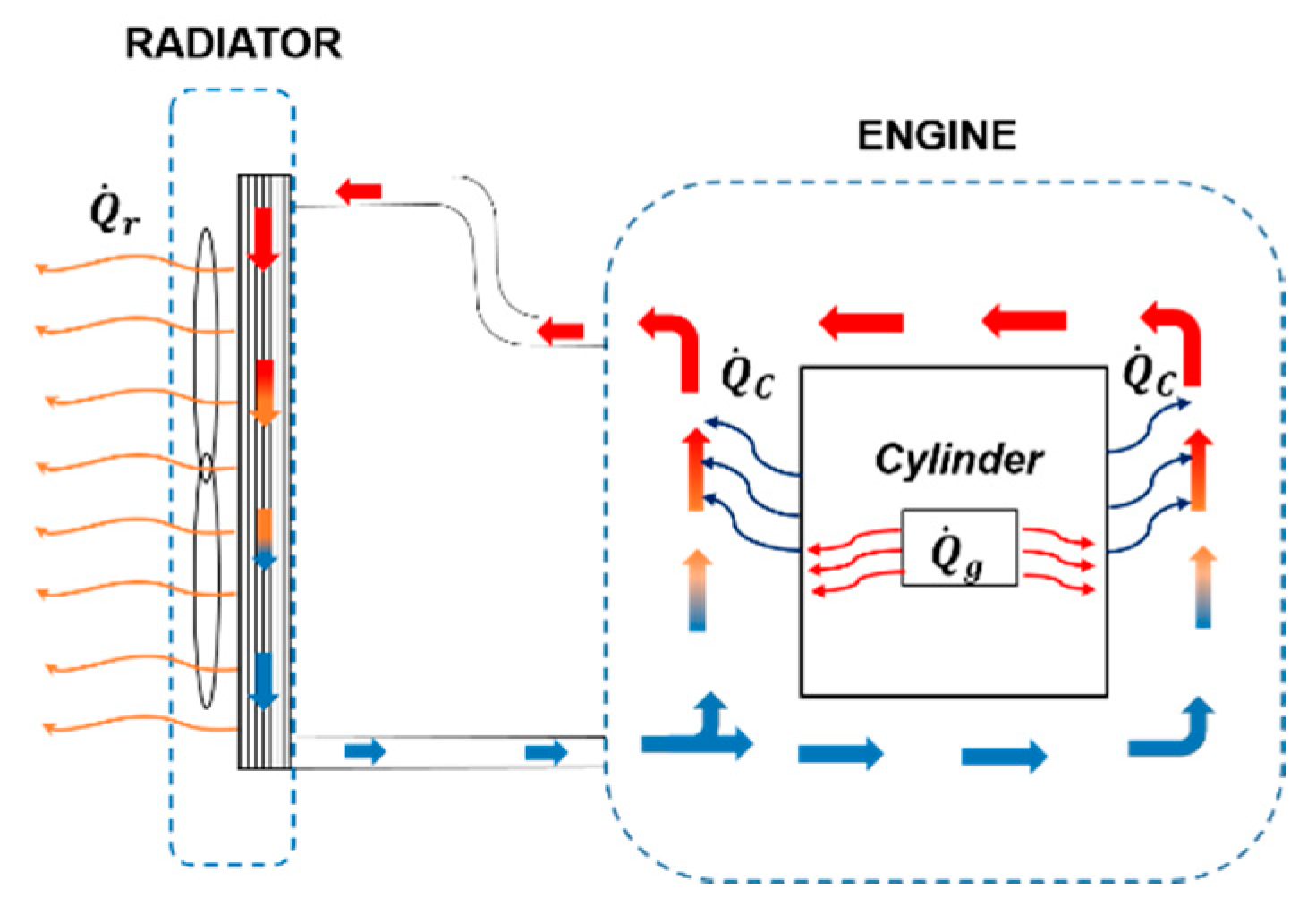
CW and CC are the engine and coolant thermal capacities. , , and are the heat transfer rates from the combustion gases to the metal, from the metal to the coolant, and from the coolant to the radiator (Figure 1).
is estimated by Equation (3) developed in [34], which includes the fuel flow rate, , the coolant flow rate, , and the engine speed, N:
The coefficients c, n, n1 and n2 were calibrated at the experimental test rig.
The heat-transfer rate to the coolant is determined by the following correlation:
which takes into account forced convection and nucleate boiling. The heat transfer coefficient, hmac, due to forced convection is modeled through the well-known Dittus–Boelter correlation [36], while for hmic, due to nucleate boiling, the Chen approach is used [37]. In Equation (4), TW is the metal temperature, is the bulk flow temperature, Tsat is the coolant saturation temperature at the given pressure, A is the total heat transfer area and Anb is the percentage of the wall area affected by the nucleate boiling. The latter is calculated as:
where qw is the actual thermal flux through the engine walls and qONB is the threshold thermal flux, which determines the nucleate boiling onset [34].
The heat transfer rate from the coolant to the atmosphere through the radiator is computed as:
where TC,out and TC,in are the coolant temperatures at the radiator inlet (engine-outlet) and radiator outlet (engine-inlet), respectively, and cp is the coolant specific heat.
Finally, an index, which indicates if boiling occurs, is defined:
Hence, if NB_Index ≤ 0 no boiling occurs; if NB_Index ⁓ 0 nucleate boiling occurs; for NB_Index ⁓ 1 saturated boiling conditions are reached. Details on the modeling equations for nucleate boiling are included in [34].
2.2. Controller Design
The coolant flow rate is the variable selected for the optimization of the engine thermal management. Other quantities, which define the engine operating point, such as the engine speed and load, are determined by the drivers’ needs; therefore, they cannot be known a priori and, from the control point of view, are considered as disturbances. However, these quantities are measured onboard and are useful for the proper functioning of the controller.
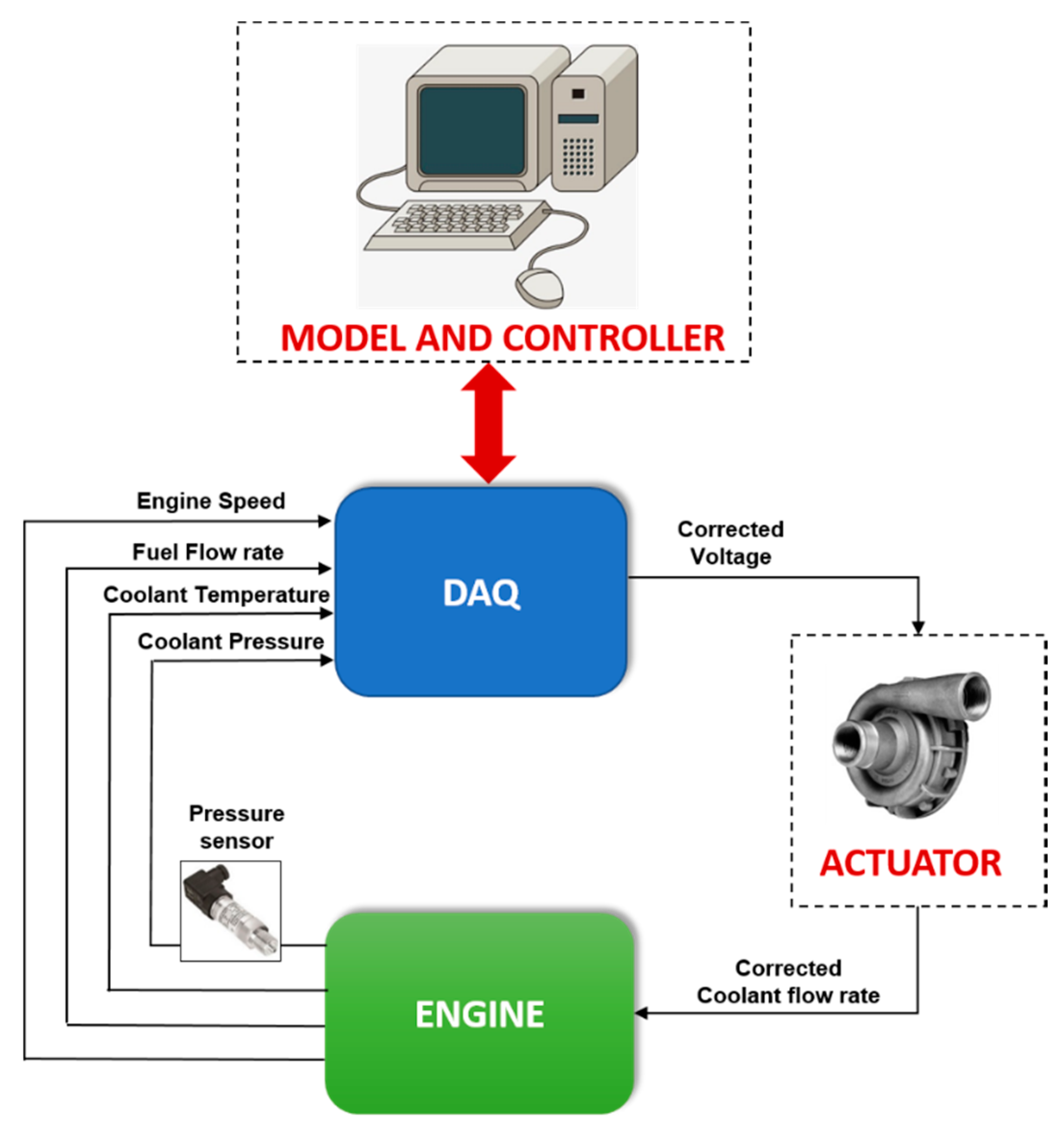
Figure 2 shows the working scheme of the controller in real-time operation at the experimental test rig. Measurements of coolant temperature at the engine outlet, of fuel flow rate and engine speed are usually available on modern engines; in addition, the proposed controller requires the measurement of coolant pressure for the detection of nucleate boiling. At each time step, the signals from transducers are sent to the data acquisition system (DAQ) and to the computing facility, where the controller is implemented. The model is used to calculate the wall and coolant temperatures, which, in turn, are used as controller inputs for the calculation of the correction to be applied to the actual coolant flow rate. This correction is then converted into a proper voltage, and hence into a proper rotational speed for the electrically driven pump, which delivers the corrected coolant flow rate to the engine. The working principle onboard a vehicle in real-time is very similar as the computing facility and the DAQ are substituted by the electronic control unit (ECU).
Figure 3 enters in more detail regarding the interaction between the model and the controller. The signals, out from engine transducers, are sent to the model, which computes the wall and coolant temperatures (TW, TC) for that particular engine operating point (Equations (1) and (2)).
These values are used by the controller to select a control region in the plane (TW, TC), which defines the state of the system. The controller, in fact, enters the state space with a couple of values (TW, TC) (Point A in Figure 3) and selects the control region, which is approximated by an ellipsoid, where the point enters. Each ellipsoid is characterized by an equilibrium coolant flow rate, , an equilibrium coolant temperature, TC,eq, an equilibrium wall temperature, TW,eq and two-state feedback control gains, K1 and K2. These characteristic values are collected and read from a look-up table and the correction to the equilibrium coolant flow rate is calculated as:
The number of control regions (ellipsoids) is determined in order to cover all the possible states of the systems and, hence, the entire range of engine operating conditions and to make sure that the behavior of the linearized model does not differ significantly from the non-linear one. The values of K1, K2, and the definition of the equilibrium values, which determine the coolant flow rate correction, are the result of an optimization problem, which is carried out off-line, during the controller design stage. The optimization problem includes the model linearization for an engine operating point, the definition of the constraints on input and output variables and the minimization of a cost function. In particular, constraints are defined for the disturbances and the output variables; for the disturbances, the constraints define the minimum and maximum expected values for engine load and speed; for the output variables, the constraints define the maximum and minimum allowed values of wall temperature, coolant temperature, and boiling level, which guarantee for instance engine reliability. Then, a cost function, which integrates the deviation of the engine parameters from the desired values is defined and the linear objective minimization problem is formulated. The solution returns the state-feedback controller gains, K1 and K2 and the controller stability region, whose shape, in the state space, is that of an ellipsoid. In conclusion, the controller acts with the aim to vary the coolant flow rate to guarantee that, as long as the disturbances are contained within prescribed constraints, the engine temperatures are kept inside the stability region of the controller, rejecting the disturbances variations and satisfying, therefore, the constraints on the output variables TW and TC and on the NB_Index.
The simulation tool developed in the present work operates following the scheme in Figure 3. In this case, the input data, instead of being read from the transducers, are read from an input file, which includes the fuel flow rate, , engine speed, N, coolant pressure, pin and coolant temperature, TC,in; these data are usually obtained from real engine operating conditions. The coolant flow rate, , is computed by the controller and is given as an input to the engine thermal model.
3. Experimental Validation
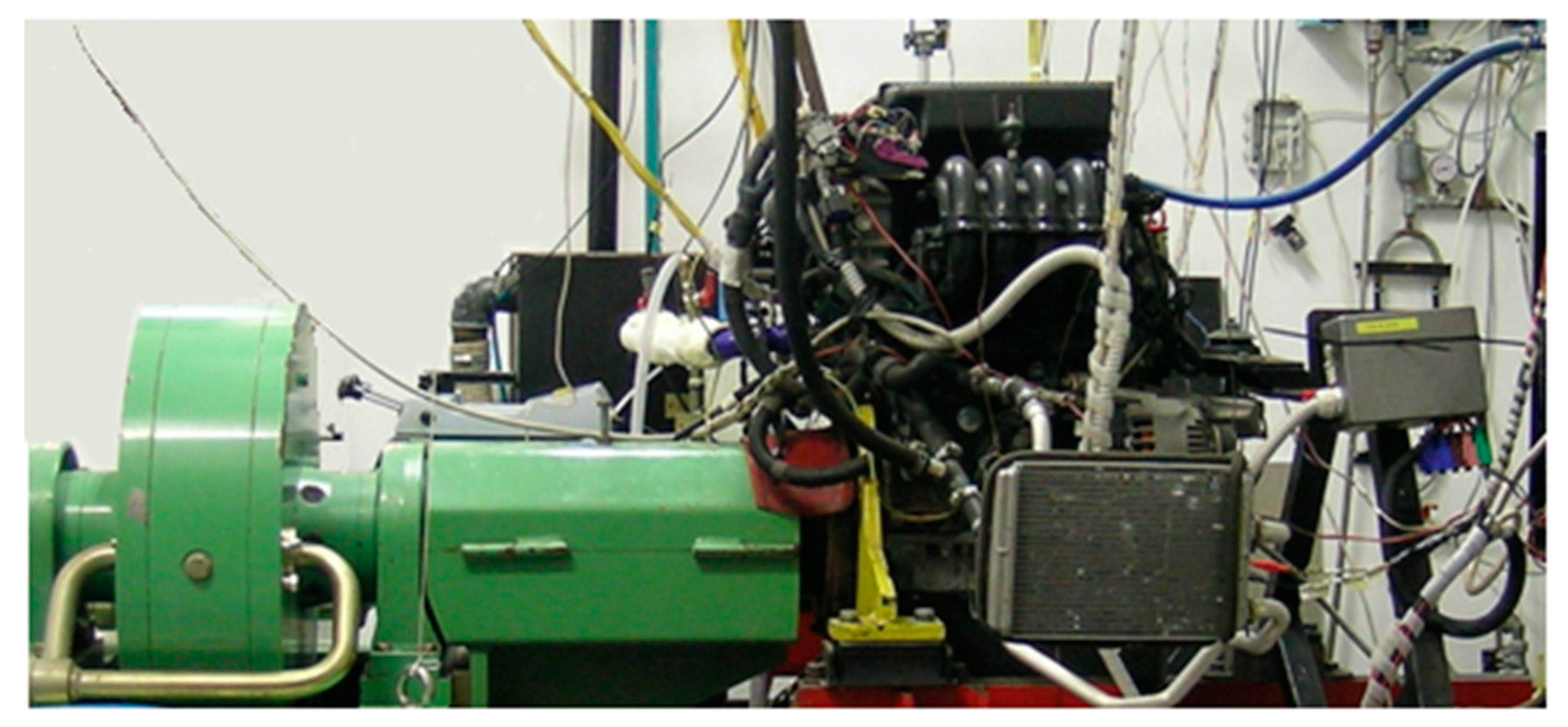
The controller is validated at the experimental test rig. Tests are carried out on a spark-ignition engine, whose displacement is 1.2 dm3; it delivers a maximum power of 60 kW between 5000 and 6000 rpm. The test bench is equipped with an eddy current engine torque dynamometer, which controls engine speed and allows load variation by setting either torque or throttle position. The fuel consumption is measured through an AVL 733S metering system; coolant pressure and temperatures at engine inlet and exit are measured by means of pressure transducers and temperature sensors (PT100-type), respectively. Figure 4 shows the experimental test rig.
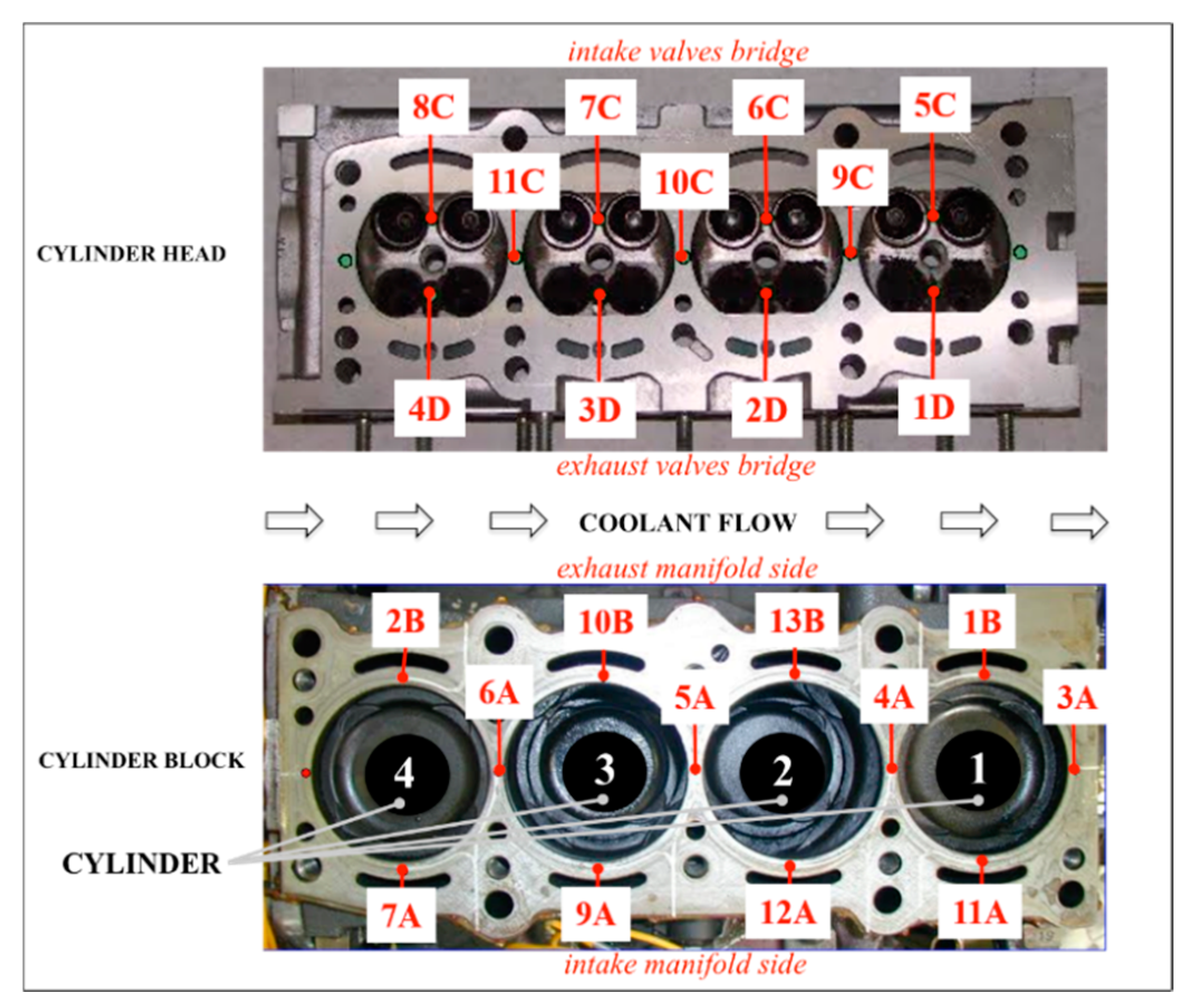
The cooling circuit layout includes an electrically driven pump manufactured by OMP, which delivers a maximum coolant flow rate of 240 dm3/min at 5000 rpm, maximum power of 1000 W, and overall efficiency of 67%. The coolant flow rate is measured by means of an electromagnetic flowmeter (Proline Promag E 100). Finally, K-type thermocouples are positioned in the cylinder head and block (Figure 5). The radiator and pressurized expansion tank are the production ones.
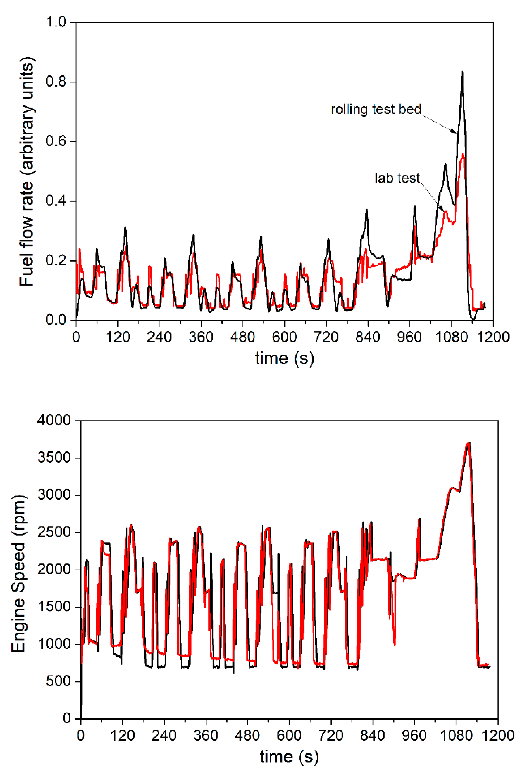
The NEDC is replicated at the stationary test bench. To this aim, the torque-speed couples of values adopted during the NEDC tests at the rolling bench have been adapted for the stationary test rig tests and have been changed into throttle opening-engine speed series of data, applied to the dyno. The fuel flow rate (in arbitrary units for the privacy policy of the engine constructor) and the engine speed from rolling test bed and stationary test rig are shown in Figure 6, where a high level of similarity between both cases is well visible.
Figure 7 shows a comparison between the average wall temperature calculated by the model and the thermocouple measurement in a specific engine head location when the controller is operating.
The agreement is satisfactory; the differences can be explained by considering that simulations are carried out by using engine speed, fuel flow rate, and coolant temperature values given by the constructor as measured at the rolling bed. On the contrary, in the current experiments, the engine speed, fuel flow rate, coolant pressure, and temperature values are those actually measured during the lab tests (Figure 6, top).
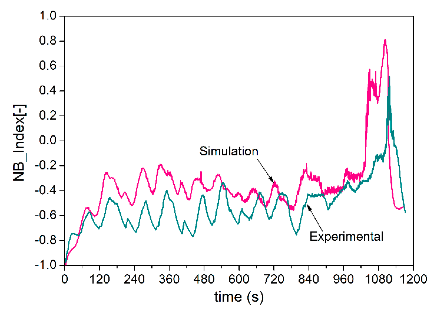
Figure 8 displays the NB_Index for both simulated and experimental controller. The results are satisfactory and simulations are in accordance with the experimental data.
Details on the controller parameters adopted for validation purposes will be described in the next section, where the results of numerical simulations carried out with three different controllers will be presented.
4. Results
The controller is designed to operate at the lowest coolant flow rate as long as the wall temperature is lower than 100 °C. In such conditions, the energy required by the pump is the lowest possible; at the same time, the engine temperature is in the range of metal reliability and the coolant is safe from boiling. After the engine wall reaches the threshold value of 100 °C, the controller adjusts the coolant flow rate determined by the ellipsoid crossed by the trajectory. In the present work, three different control strategies are developed: in the first case, a low nucleate boiling level of the coolant is allowed; in the second case, the allowed boiling level is the same as the one obtained when the standard belt-driven pump operates; finally, a slightly higher boiling level is admitted. The tests are carried out for the New European Driving Cycle (NEDC), for which experimental data of fuel flow rate and engine speed for the current engine are supplied by the manufacturer (Figure 6).
4.1. Controller with Low Boiling Levels
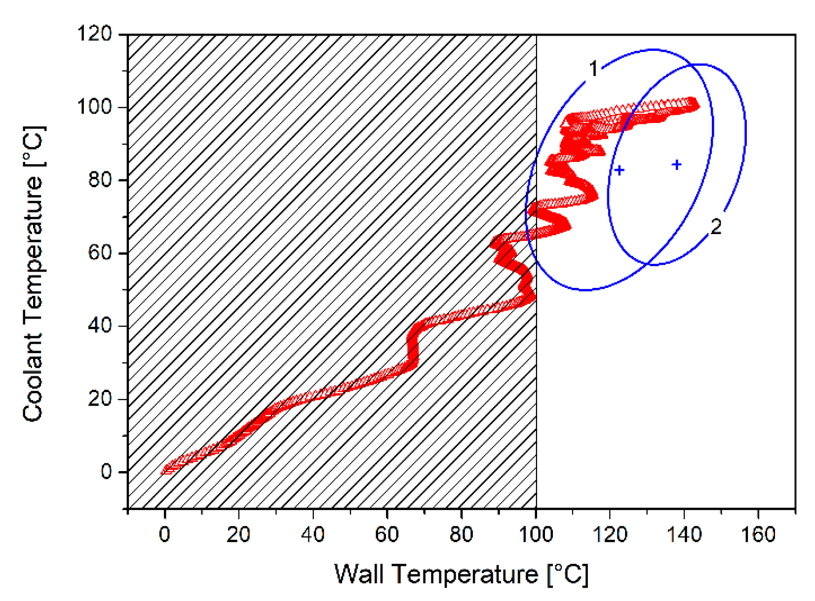
The control region and the evolution of the state of the system during the NEDC are plotted in Figure 9.
The initial wall and coolant temperature are the ambient values corresponding to 20 °C. In the dashed area, where the wall temperature is lower than 100 °C, the coolant flow rate is the lowest (~180 dm3/h) and the wall and coolant temperature vary according to the fuel flow rate enforced during the low part of the NEDC. When the wall temperature rises to reach 100 °C, the trajectory crosses the ellipsoid and the coolant flow rate is modified to satisfy the controller constraints for the selected ellipsoid.
The constraints for Ellipsoid No.1 are summarized in Table 1. The constraints on fuel flow rate and engine speed are given by the NEDC; the maximum fuel flow rate, , is about 9 kg/h and the engine speed can vary in the range 500–4000 rpm. The maximum coolant flow rate, , is determined by the pump, which delivers about 6000 dm3/h. Finally, the constraints on the output variables are defined by the constructor. If a moderate boiling level is required (NB_Indexmax = 0.3), with an average pressure of 1.4 bar, a maximum average coolant temperature of TC of 110 °C and a maximum average wall temperature TW of 160 °C can be achieved.
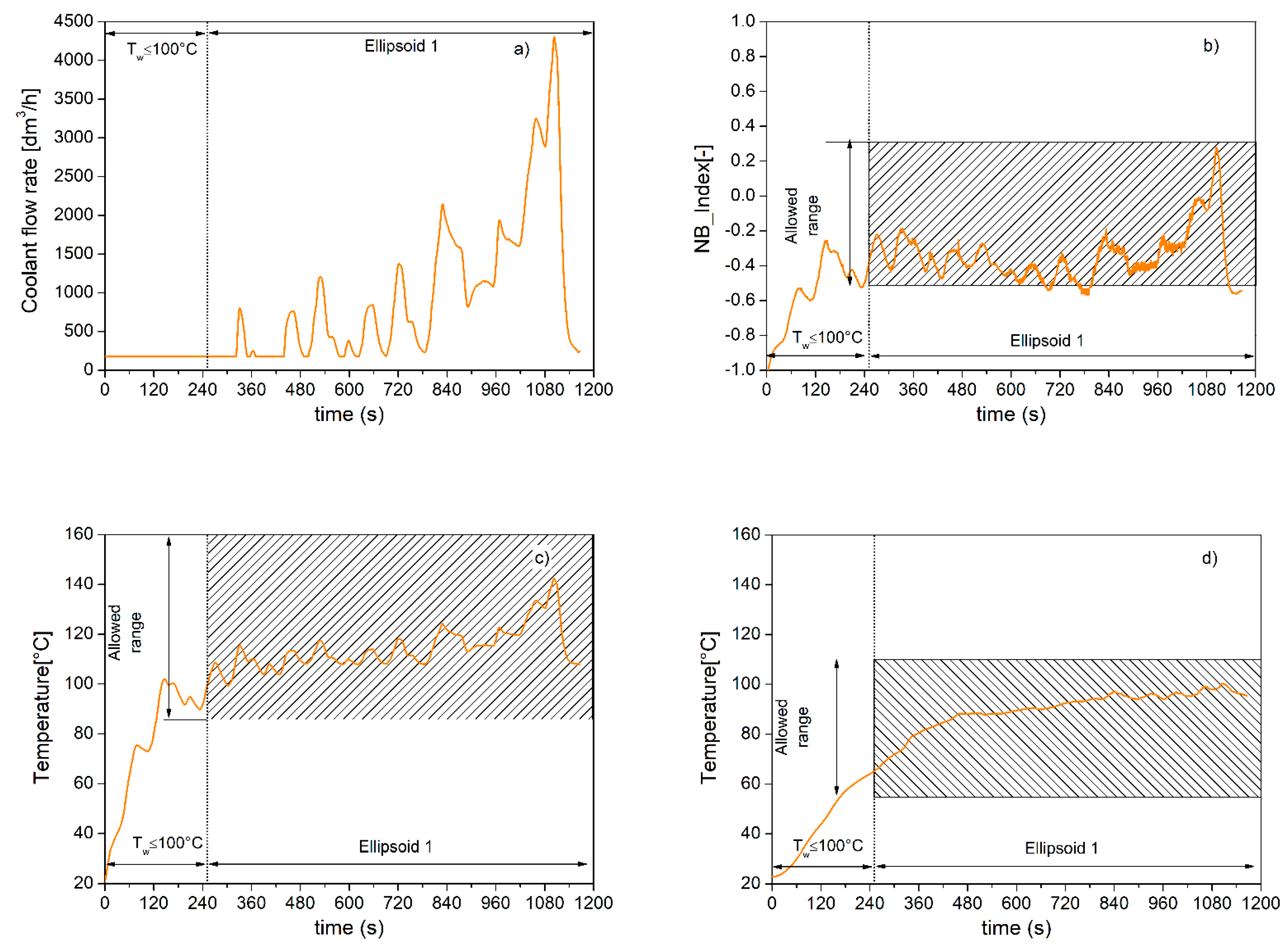
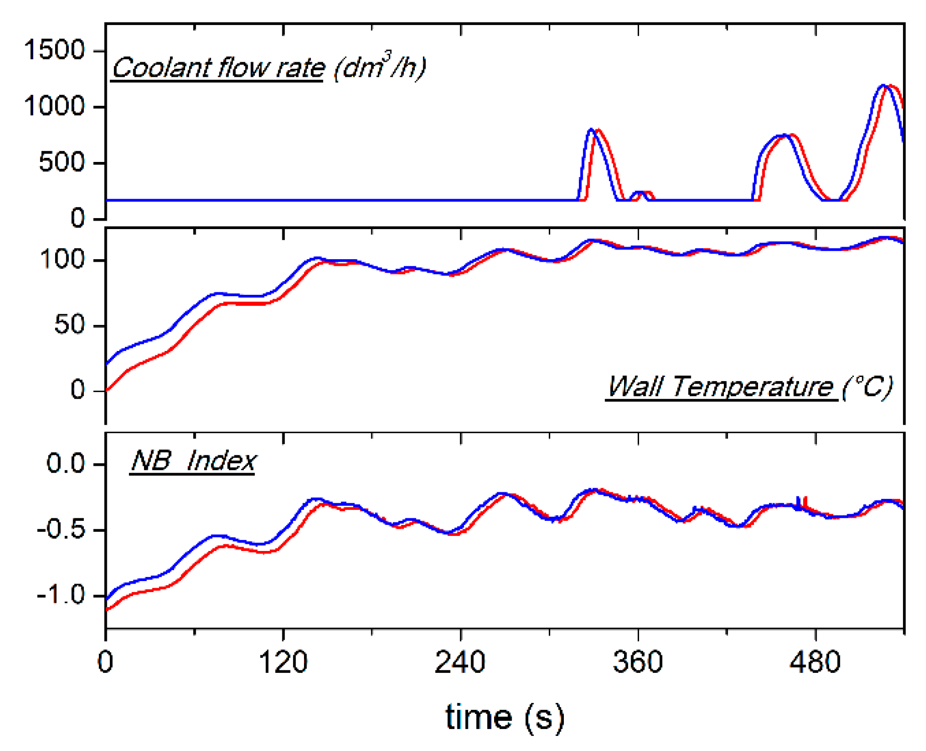
The resulting coolant flow rate during the NEDC is displayed in Figure 10a. It can be observed that, as long as the wall temperature is lower than 100 °C (Figure 10c), the pump delivers the lowest coolant flow rate and no boiling occurs (Figure 10b) owing to the low metal and coolant temperatures achieved in this operating range (Figure 10c). When the threshold wall temperature is exceeded, the state of the system crosses Ellipsoid No.1 (Figure 9) and the coolant flow rate varies in order to satisfy the controller constraints whilst the fuel flow rate and engine speed vary according to Figure 6. Figure 10c,d shows that both the wall and coolant temperatures are kept within the prescribed ranges. At the same time, the NB_Index is lower than the maximum allowed value (Figure 10b).
4.2. Controller with Moderate Boiling Levels
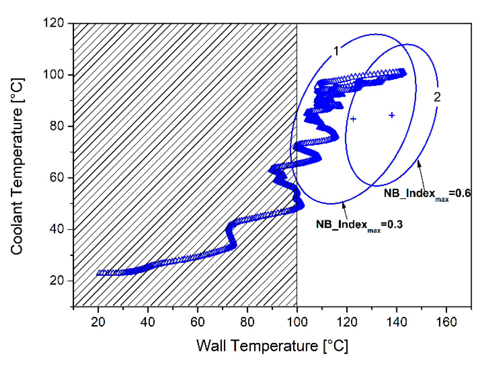
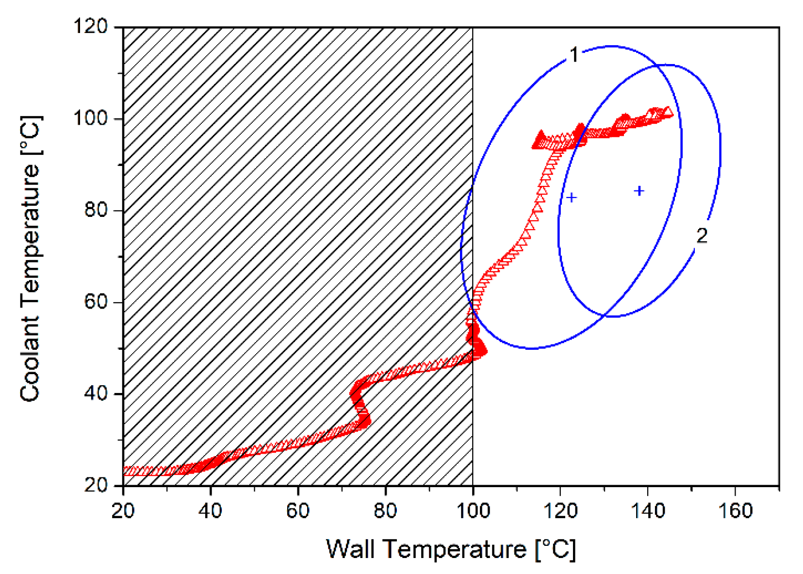
If moderate boiling levels are allowed, like the ones that occur when the standard belt-driven pump is adopted (NB_Index ~ 0.5/0.6), a new controller can be adopted. In this case, a new control region with a higher NB_Index is obtained with lower coolant flow rates, which increase the wall and coolant temperatures and move the equilibrium point towards higher values (Ellipsoid No.2). The control region is, however, smaller than the previous one (Ellipsoid No.1), owing to the constraints on the maximum wall and coolant temperatures, which are substantially unchanged when compared to the previous case. As Ellipsoid No.2 is not large enough to cover the gap with the dashed area, a transition region (Ellipsoid No.1) is, however, needed and the controller is made up of two ellipsoids, as displayed in Figure 11. When the system state (TW, TC) is in the region, which belongs to both ellipsoids, Ellipsoid No.2 is used.
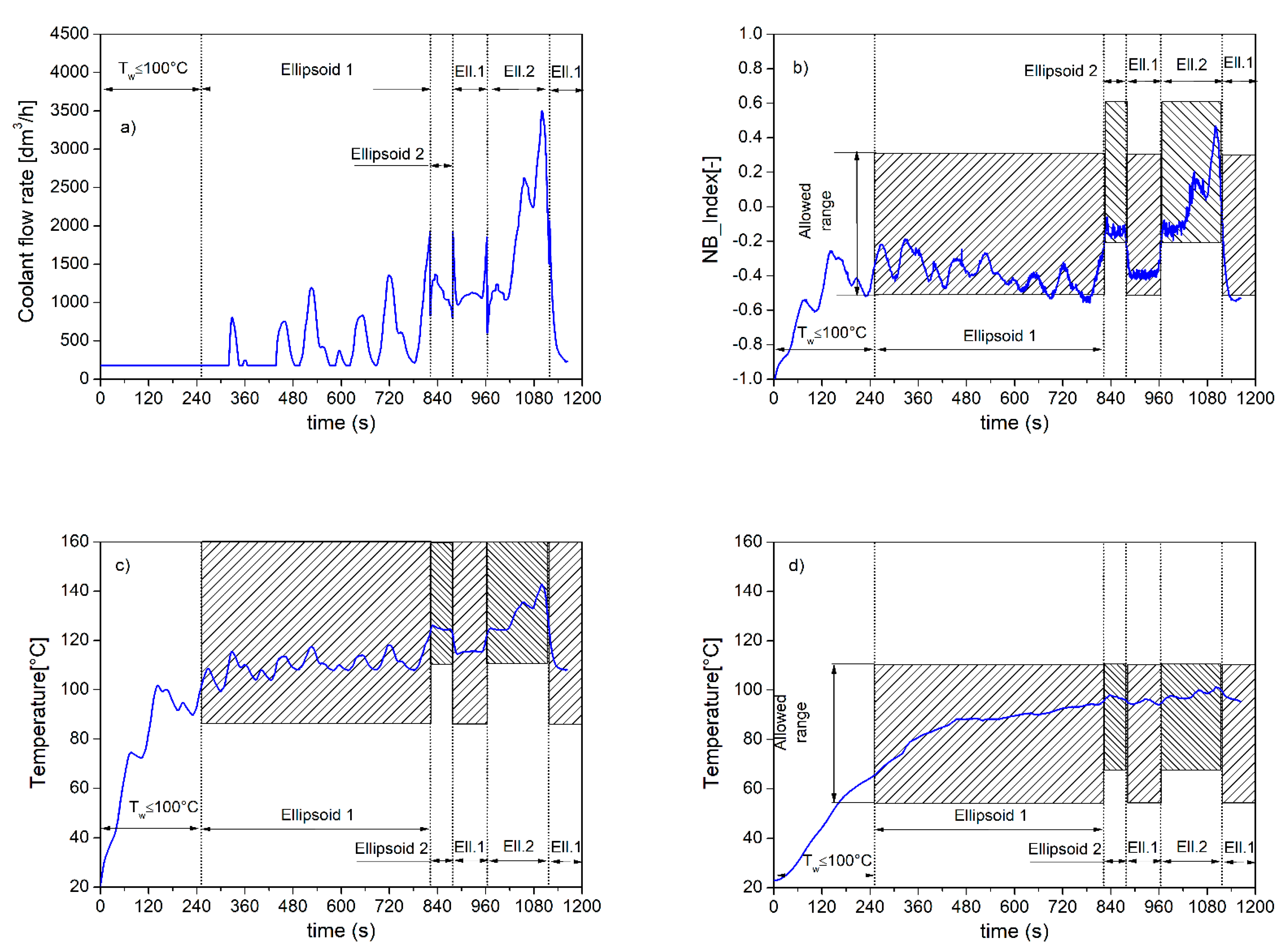
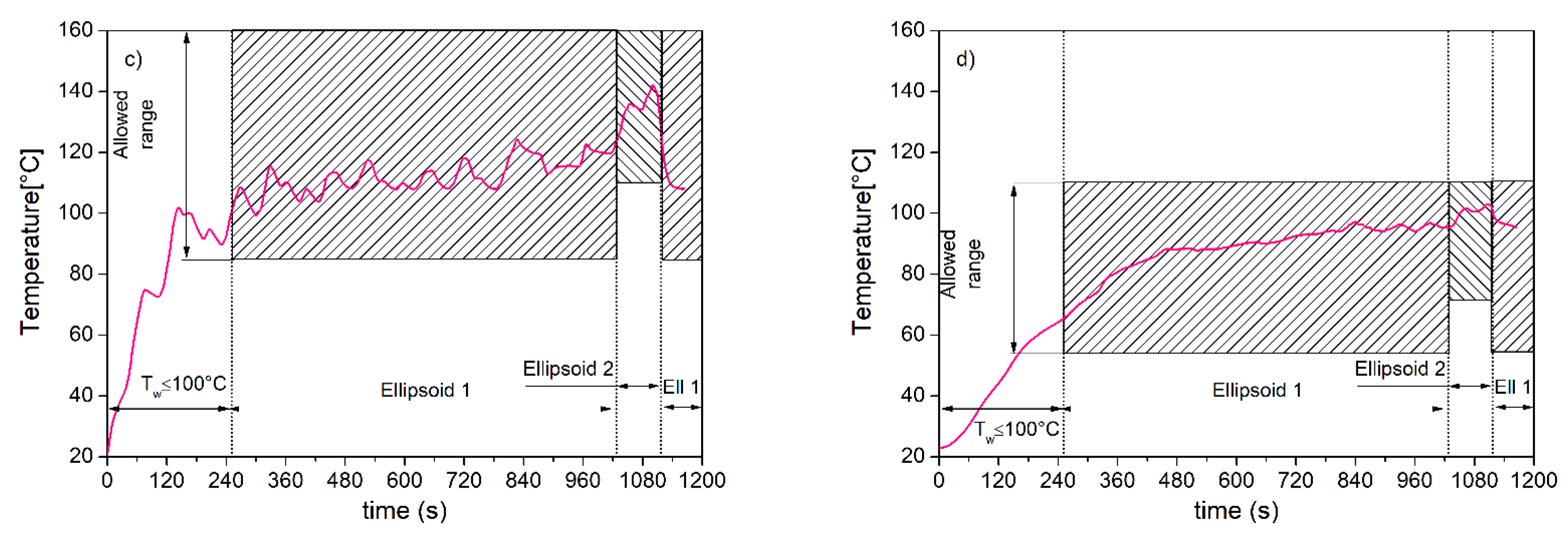
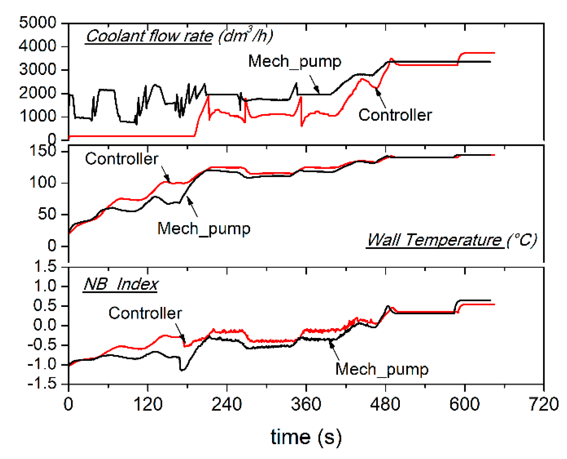
The equilibrium values and the constraints for the moderate boiling controller are summarized in Table 2. The results in terms of coolant flow rate, wall and coolant temperature, and NB_Index are displayed in Figure 12. As long as the state of the system lies in Ellipsoid No.1, no differences occur with respect to the previous case. Owing to the fuel flow rate increase, at time 822 s, the state of the system crosses Ellipsoid No.2; as this controller allows higher boiling levels than Ellipsoid No.1, the coolant flow rate decreases, while the wall and coolant temperatures and the NB_Index rise. The state of the system remains in this controller region for about 60 s before returning to Ellipsoid No.1, owing to the reduced fuel flow rate. In this region, the coolant flow rate tends to increase and to lower the temperatures; however, as the fuel flow rate is reduced, no significant variations in coolant flow rate occur. In the final part of the NEDC cycle, where the fuel flow rate increases significantly, the state of the system crosses Ellipsoid No.2 again and the coolant flow rate increases considerably; the wall and coolant temperatures and the boiling levels are kept within the prescribed limits. The effectiveness of the controller is demonstrated for the whole NEDC cycle, where the constraints on the variables are satisfied, as displayed by the dashed areas in Figure 12b–d.
4.3. Controller with High Boiling Levels
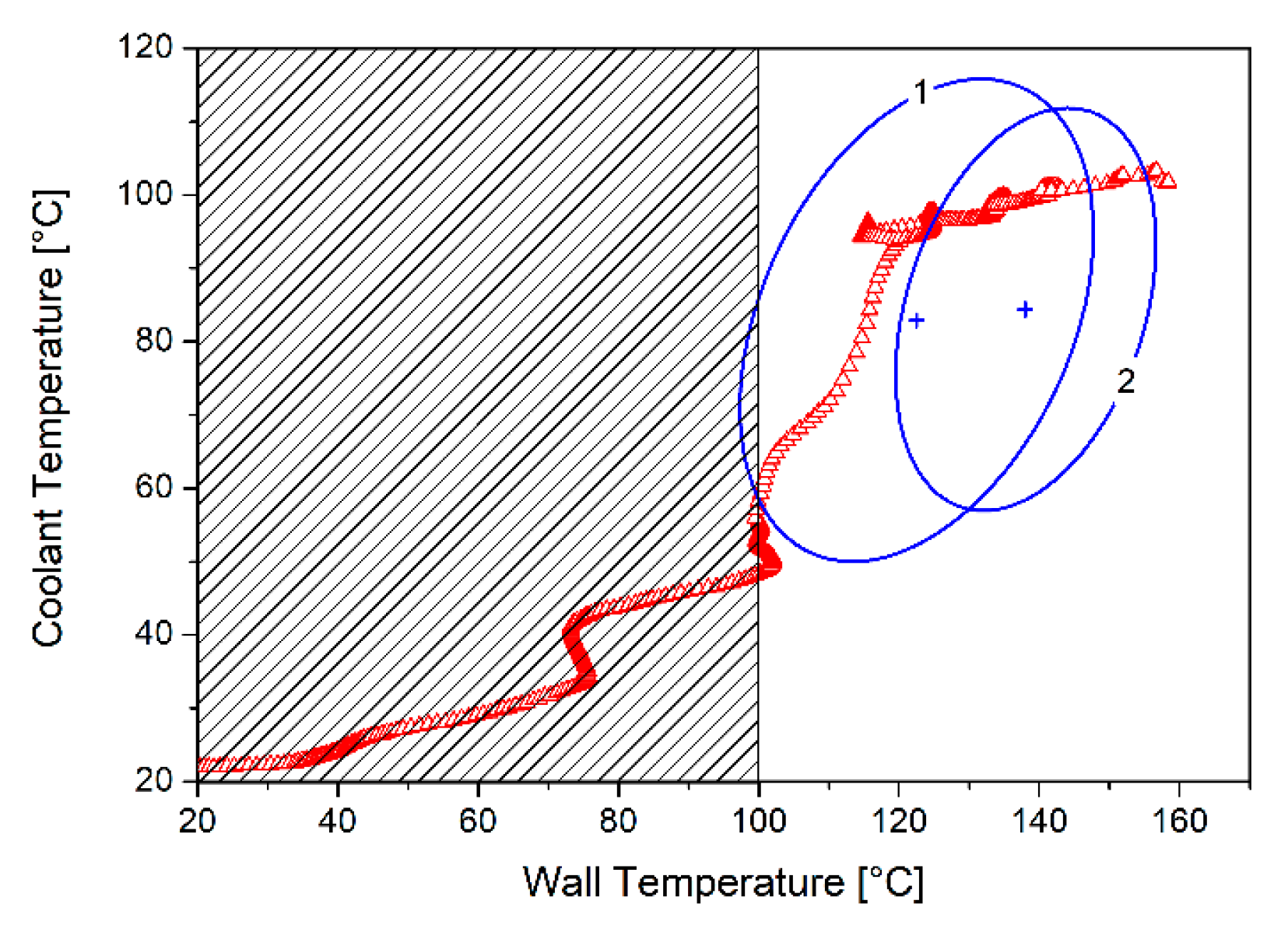
If higher boiling levels are accepted, Ellipsoid No.2 can be further modified and a new equilibrium point with a higher NB_Index can be designed (Table 3).
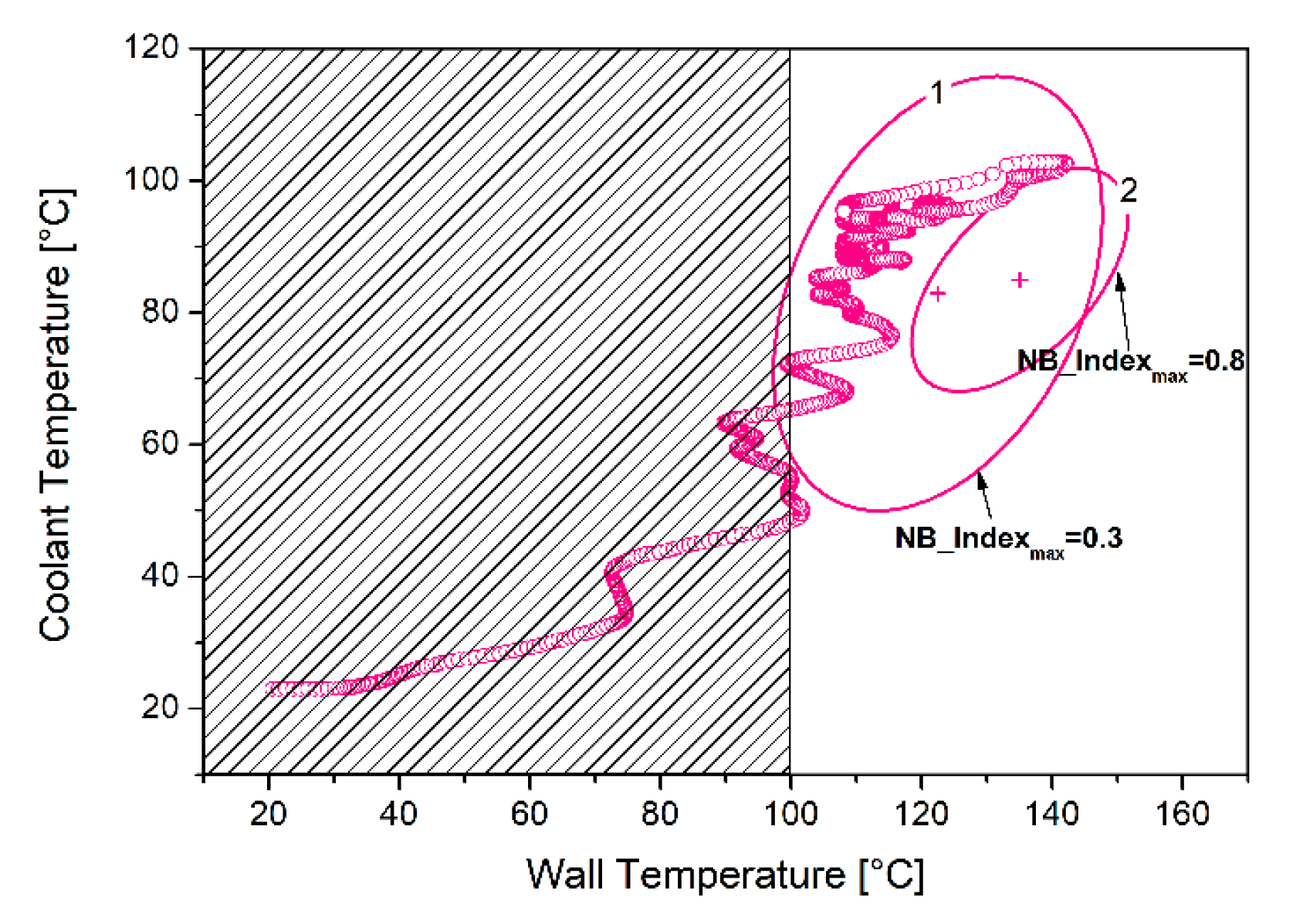
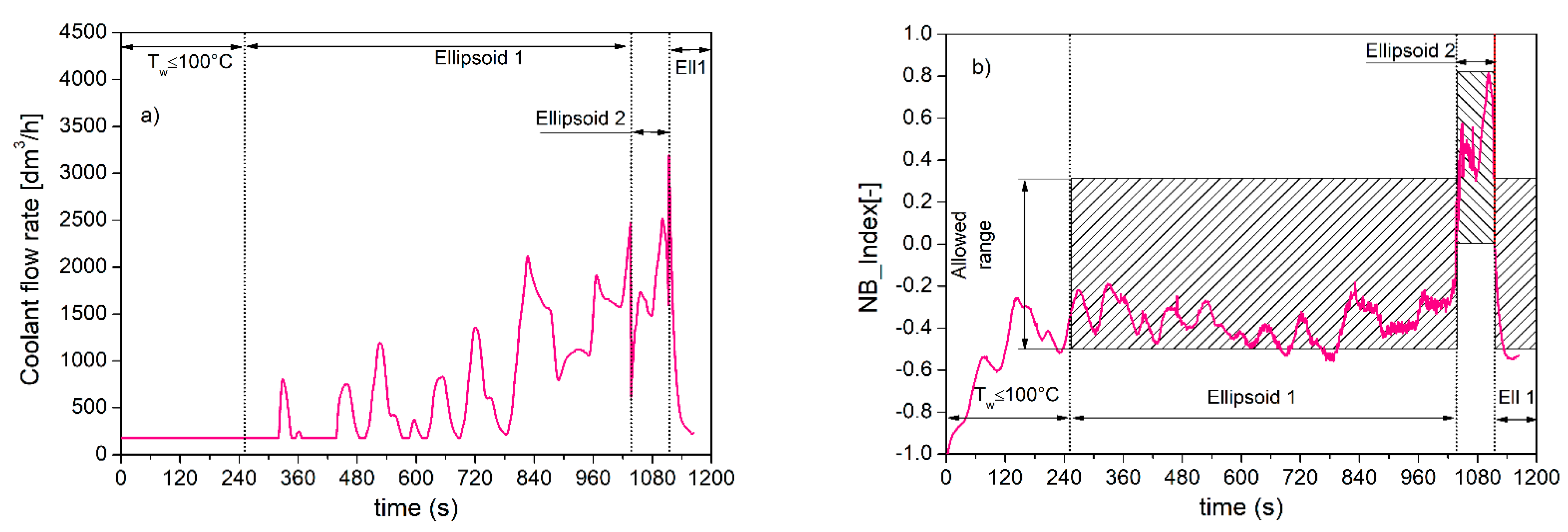
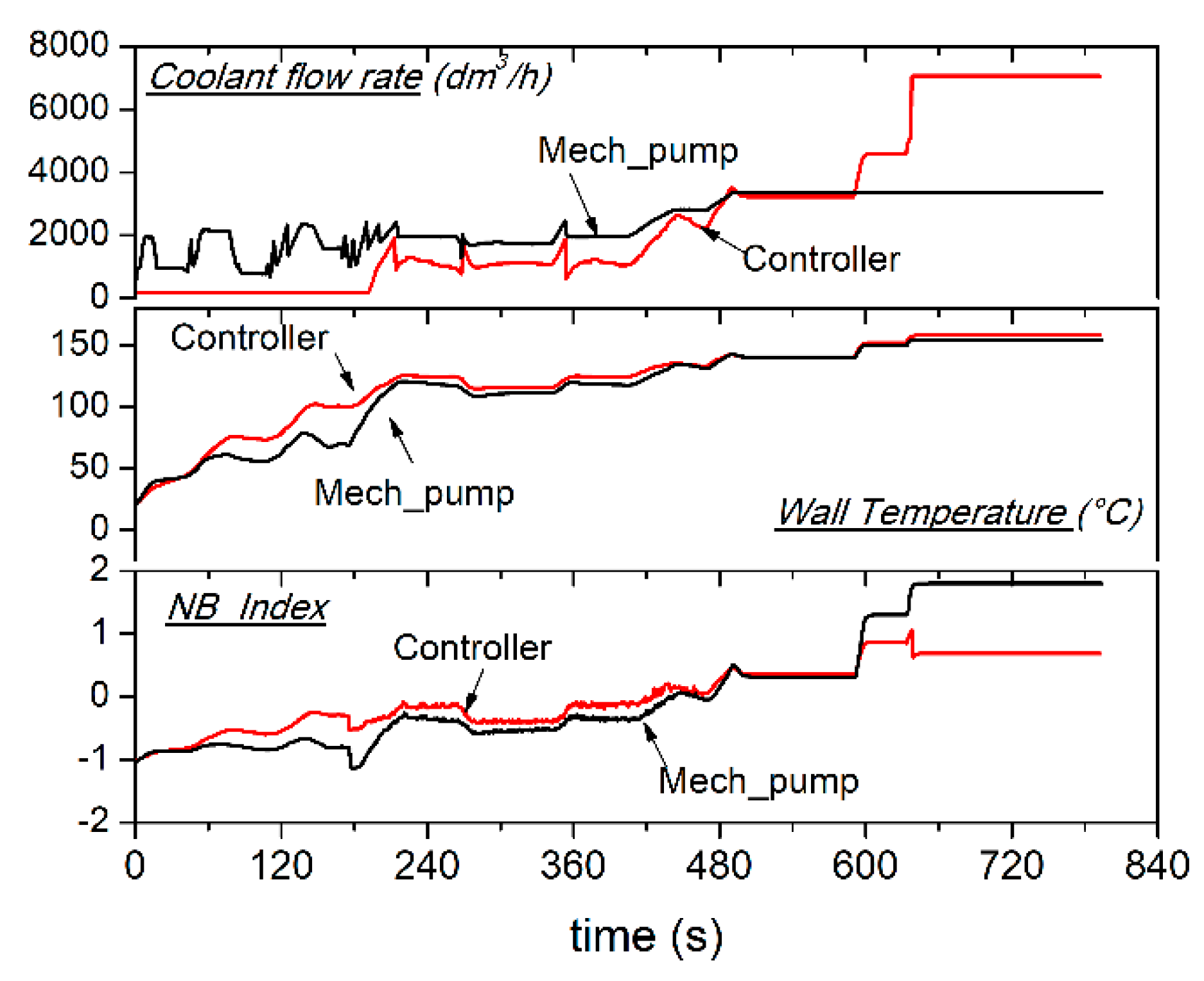
The maximum boiling level considered in the present case is about 0.8; the new controller is displayed in Figure 13 and the corresponding coolant flow rate, wall and coolant temperatures, and NB_Index are shown in Figure 14. As the state of the system crosses Ellipsoid No.2, the coolant flow rate is reduced as higher temperatures are allowed; at the same time the NB_Index increases and, at the highest fuel flow rate, it reaches, without exceeding, the maximum allowed value.
4.4. Comparison with the Belt Driven Pump
A comparison of the adoption of the standard belt-driven pump and the electrically driven pump with the developed controllers is presented in this section. In the following figures, the controllers with low, medium and high boiling levels will be denoted as Controller A, B, and C, respectively.
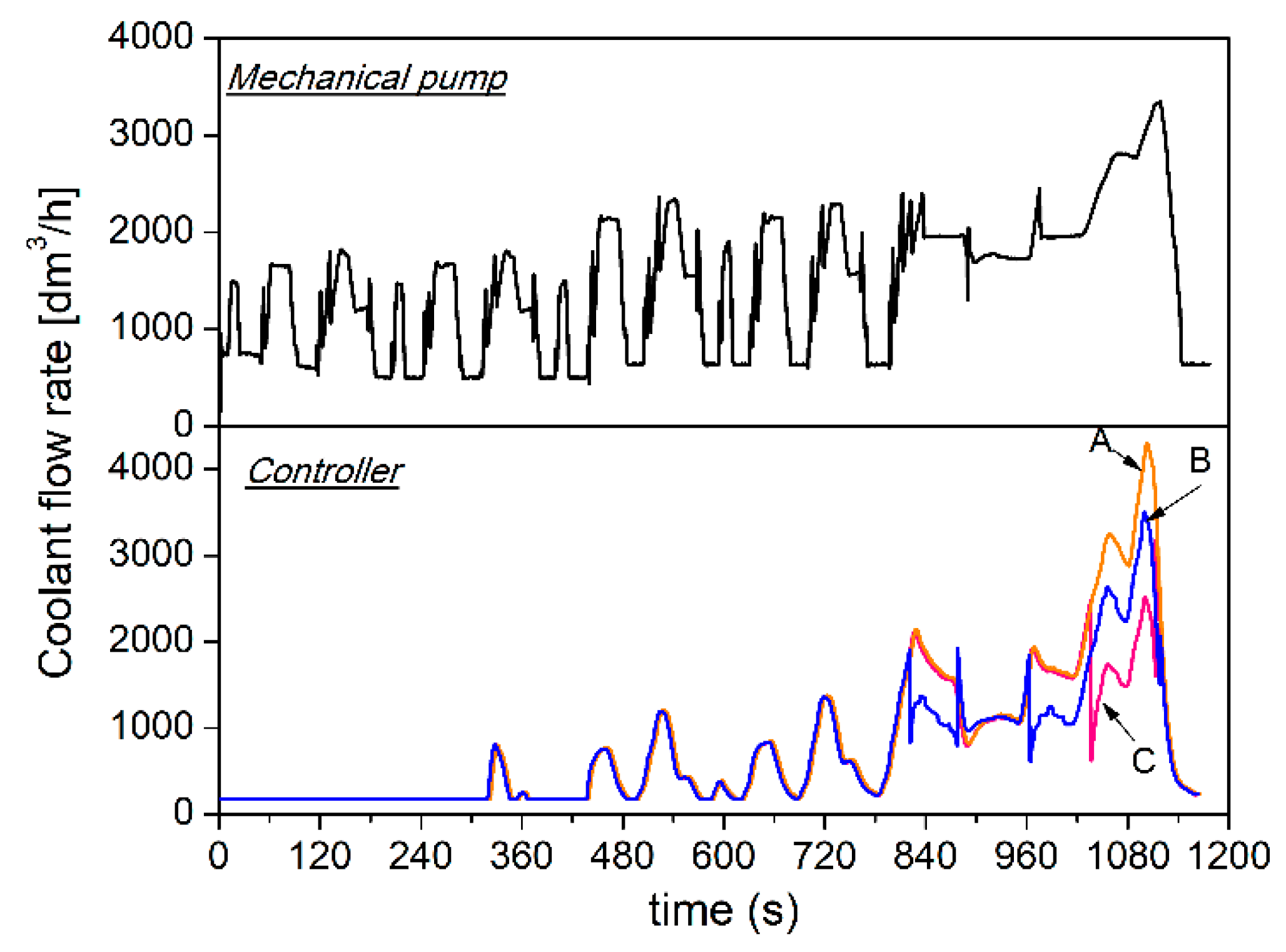
Figure 15 displays a comparison between the coolant flow rate as obtained with the crankshaft-driven pump (top) and with the controllers (bottom). In the urban part of the cycle (time ~ 770 s), the standard belt-driven pump delivers a considerably higher coolant flow rate (800 ÷ 2000 dm3/h) than the controller (176 ÷ 1000 dm3/h), while no difference occurs among the various controllers. In fact, Ellipsoid No.1, which acts in this part of the cycle, is the same for the three controllers. In the extra-urban part of the NEDC, the coolant flow rate increases for all cases. The highest coolant flow rate, even higher than the belt-driven pump, is delivered by Controller A, which allows low boiling levels, while Controller C, which allows a higher degree of boiling, reduces considerably the coolant flow rates in this part of the cycle.
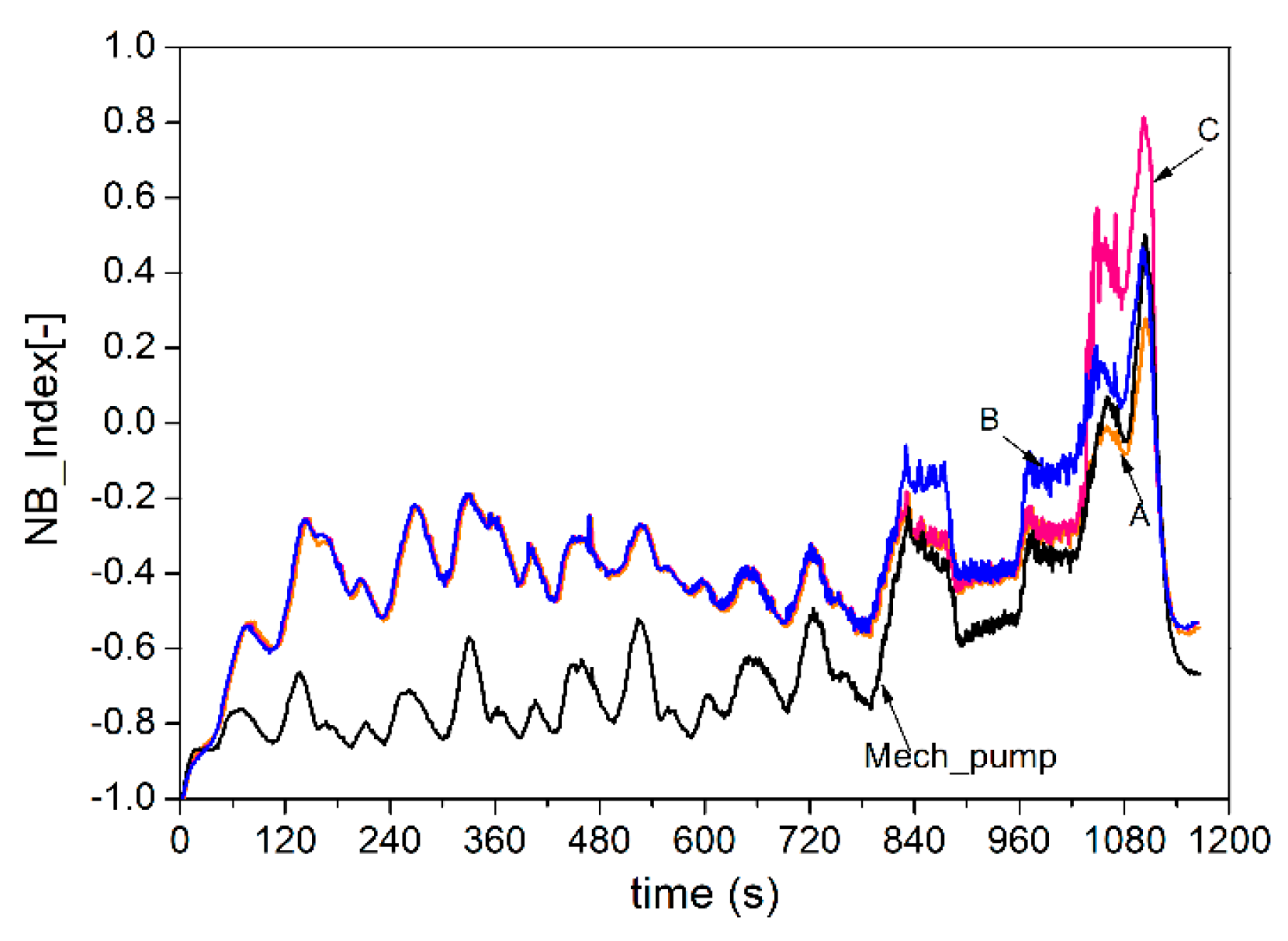
The boiling levels are plotted in Figure 16 for all the cases. The figure shows that, in the urban part of the NEDC (time ~ 770s), the mechanical pump overcools the engine; the lower coolant flow rate delivered by the controller enhances NB_Index, which is, however, negative and the coolant is safe from boiling. In the extra-urban part of the cycle, the boiling level starts to increase and, with the adoption of the mechanical pump, the maximum level of boiling is NB_Index ~ 0.5. Controller A limits the NB_Index at 0.3, Controller B allows the same boiling level as the belt-driven pump and Controller C slightly enhances this limit.
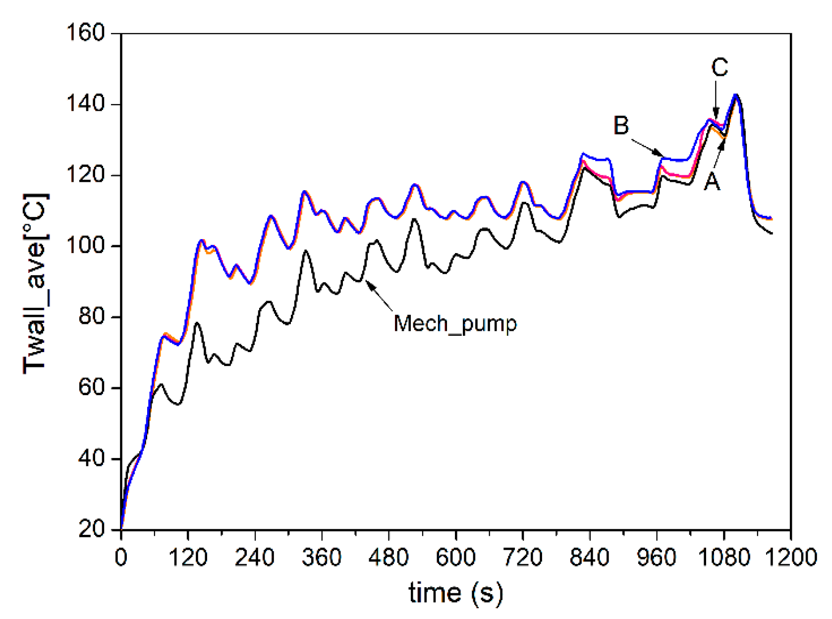
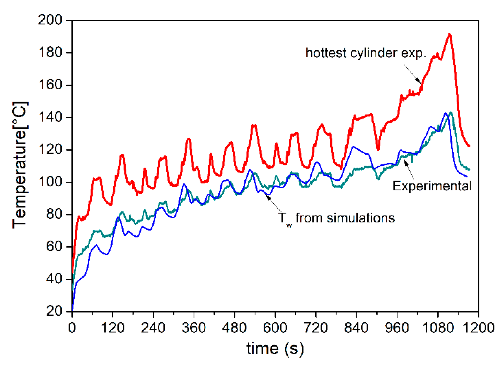
The boiling levels, however, preserve the engine metal, whose average temperature during the NEDC cycle is plotted in Figure 17. The figure shows that, despite the adoption of lower coolant flow rates, in the hottest part of the cycle the temperatures are well within the reliability limits. The analysis is carried out over the average wall temperature; it is, however, worth pointing out that, from the experimental data, the difference between the average metal temperature and the hottest thermocouple is about 40 °C, as displayed in Figure 18, and is still in the metal reliability range.
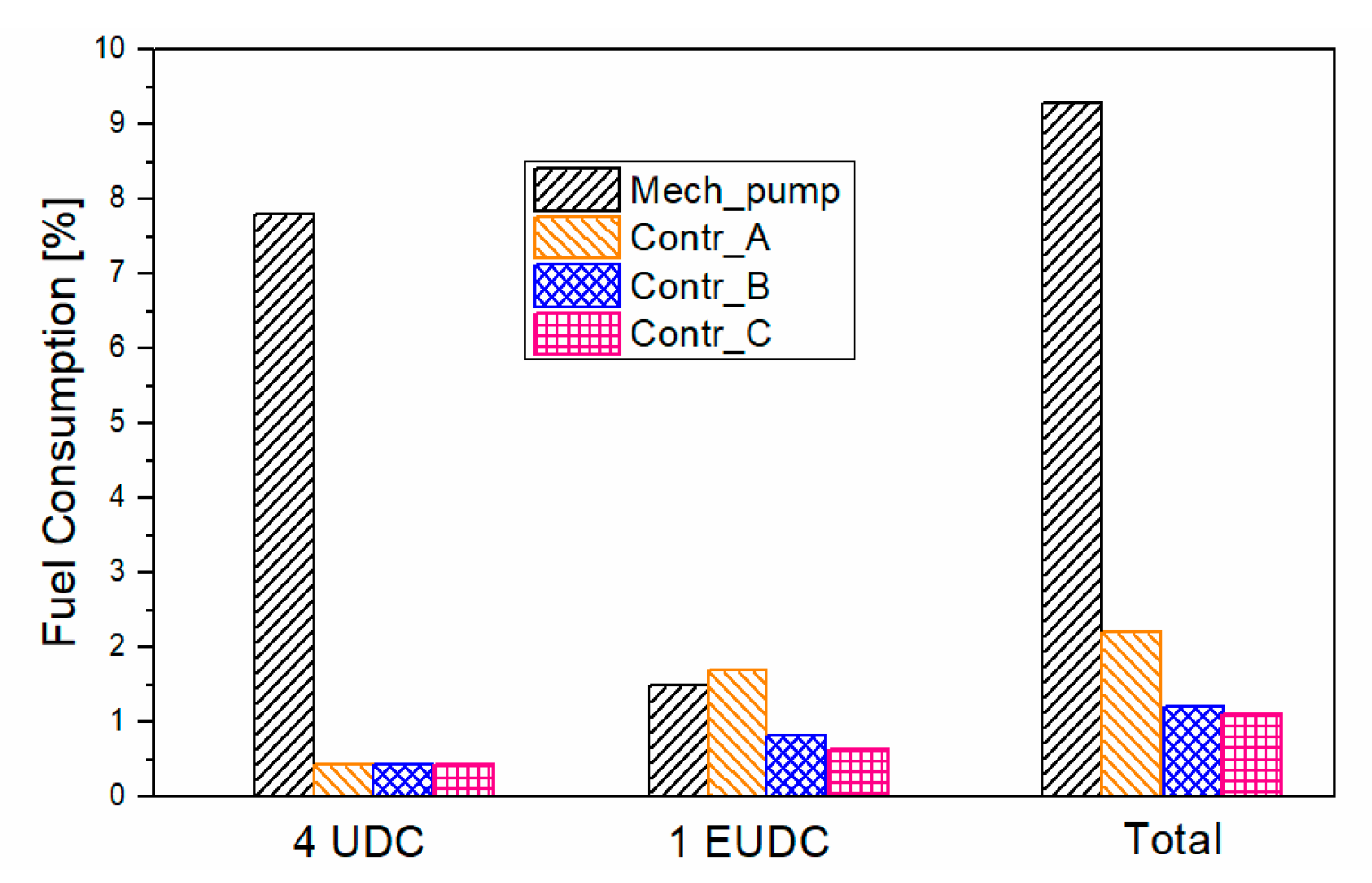
A final comparison regards the fuel economy related to the adoption of the controller. The results are summarized in Figure 19. The amount of fuel consumed to actuate the belt-driven pump is about 9.3% of the fuel consumed over the entire NEDC cycle. The largest amount is consumed during the four urban driving cycles (7.8%) and the remaining 1.5% is consumed during the extra-urban driving cycle. When the controller is adopted, the fuel consumption due to the actuation of the electrically driven pump is considerably lowered. If the controller with low boiling levels is adopted (Controller A), the total fuel consumption for pump actuation is reduced from 9.3% to 2.1%, with a fuel-saving of about 7.2%. In this case, only a very small amount of fuel is consumed during the urban part of the cycle (~0.42%), owing to the low coolant flow rate adopted; the remaining 1.7% is consumed during the extra-urban cycle, where the coolant flow rate rises. For the case of the controller, which allows the same boiling level as the mechanical pump, namely Controller B, the total fuel consumption for pump actuation is reduced to 1.2%, i.e., 8.1% less than the standard belt-driven pump. The fuel consumed during the urban cycle is the same as Controller A (~0.42%), where the coolant flow rate is the minimum, while a significant reduction occurs in the extra-urban cycle, where a fuel consumption of about 0.8% is achieved. Finally, when the controller with the highest boiling level is adopted (Controller C), the fuel consumption for pump actuation is the lowest; in this case, the fuel consumption is reduced at 1.1% of the total fuel consumed in the NEDC. The fuel consumed during the UDC is about 0.4%, which is the same as the previous cases, while it reduces to 0.7% in the EUDC, where the coolant flow rate is the lowest when compared to the other cases.
The results in terms of fuel economy are reported in Table 4. From the above considerations, Controller B is the most effective, as it allows the achievement of the same boiling level as the belt-driven pump, with a significant fuel economy. This controller will be, therefore, taken into consideration for evaluating its performance for the engine operating under different conditions from the NEDC cycle.
5. Other Test Cases
The selected controller (Controller B) is tested under various operating conditions, which differ from the NEDC cycle, in order to assess its robustness during real engine operations. The operating conditions include the cold start (wall and coolant temperatures starting from 0 °C and from −20 °C), a prolonged high load operation with a maximum fuel flow rate of 9.0 kg/h and a prolonged high load operation with a maximum fuel flow rate of 18.0 kg/h.
5.1. NEDC with TC0 = 0 °C and TW0 = 0 °C
The controller is applied to the engine, which performs the NEDC in a typical winter environment where the starting temperatures are about 0 °C. The controller output is plotted in Figure 20, which shows that, even though the wall and coolant temperatures start from 0 °C, the trajectory falls inside the control regions, and no further ellipsoids, for covering different engine operating points, are needed.
The desired specifications of the controller are satisfied also in this case, as displayed in Figure 21. In particular, the main difference with the previous case, where an ambient temperature of 20 °C was considered (Section 4.2), occurs for the wall temperature and for the NB_Index in the early 160 s of the cycle; after that time interval, the two cases practically overlap.
5.2. One Urban Driving Cycle and One Extra-Urban Driving Cycle with Prolonged High Load Operation at = 9 kg/h
The case where the engine performs one urban driving cycle, one extra-urban cycle and is then kept at high load operation (constant fuel flow rate and engine speed) for about 60 s, is simulated (Figure 22). The maximum fuel flow rate during the extra-urban cycle is about 9 kg/h; this value is the upper limit of the constraint on the fuel flow rate during the controller design procedure (Table 2). The engine speed is 3700 rpm.
Figure 23 shows that, also for this case, the trajectory falls inside the control regions owing to the fact that the constraints on the input variables, mainly the one on fuel flow rate, are satisfied.
The results in terms of coolant flow rate, wall temperature, and NB_Index are displayed in Figure 24, where a comparison with the crankshaft-driven pump is also included. As expected, the controller allows the adoption of lower coolant flow rates than the mechanically driven pump; however, during the high load operation, the coolant flow rate is blocked at a value of 3300 dm3/h (at 3700 rpm) for the belt-driven pump, while it increases at 3800 dm3/h for the controlled pump. Despite the wall temperature levels being almost the same, the NB_Index exceeds the upper limit of 0.6 in the case of the belt-driven pump, while it remains in the prescribed limits with the controller (NB_Index = 0.55).
5.3. One Urban Driving Cycle and One Extra-Urban Driving Cycle with Prolonged High Load operation at = 18 kg/h
The last simulated case is similar to the previous one, except for the high load operation. In this case, in fact, the fuel flow rate is fixed at about 18 kg/h, far beyond the engine operating range and the controller design constraints; this case is presented only for an illustrative purpose and is not a realistic case.
As Figure 25 shows, at high load operation the trajectory exceeds the ellipsoids borders, indicating therefore that, as the constraints on the input variables are not satisfied, the controller is not able to guarantee that the coolant flow rate is adequately corrected. In fact, Figure 26 shows that, during the high load operation, the controller enforces the highest possible coolant flow rate allowed by the actuator (~7000 dm3/h); this value is higher by the one fixed by the belt-driven pump, which at 3700 rpm delivers a coolant flow rate of about 3300 dm3/h. The metal temperatures are similar for both cases, while a relevant difference occurs in the NB_Index. With the belt-driven pump, a severe boiling occurs (NB_Index ~ 1.8); the controller contributes to reducing considerably this value to about 0.7, which, however, slightly overcomes the maximum allowed value (NB_Index = 0.6).
6. Discussion
The novel approach was validated at the experimental test rig during a standard driving homologation cycle and its effectiveness was demonstrated. Several control strategies were simulated, with three different allowable boiling levels. In particular, a controller, which allows a lower boiling level (NB_Indexmax = 0.3) than the one reached with the belt-driven pump under the same engine operating conditions (NB_Indexmax = 0.6) was first analyzed. Then, a second controller, which permits the same boiling level as the one achieved with the belt-driven pump (NB_Indexmax = 0.6) was simulated. Finally, a controller which tolerates a maximum boiling level of about NB_Indexmax = 0.8 was tested.
The findings can be summarized as follows:
- Increasing the allowed boiling level determines lower coolant flow rates; the metal temperatures are always kept inside the defined reliability limits.
- A reduced coolant flow rate under part-load conditions generally reduces fuel consumption. The 1.2 dm3 engine considered burns about 500 g during the NEDC and about 9.3% of this fuel is spent for the mechanical pump, while the fuel consumption for the electric pump, in the case of the low boiling level controller (NB_Indexmax = 0.3), is about 2%; the fuel-saving is therefore in the order of 7%. The benefit increases for the case of the high boiling level controller, when about 1.1% of the fuel is used by the electric pump and a fuel-saving of about 8% is achieved.
- The benefits of the proposed approach also occur under prolonged high-load, moderate-engine speed conditions in terms of engine reliability. In these conditions, in fact, the controlled electric pump delivers considerably higher coolant flow rates than the standard belt-driven pump and keeps the boiling levels within the safety limits (NB_Index = 0.7, in contrast with NB_Index > 1 for the case of the belt-driven pump).
7. Conclusions
In this work, a tool for designing a controller for the optimal thermal management of a spark-ignition engine was presented. The proposed approach aims at improving the engine efficiency for all those cases where the traditional belt-driven pump determines engine overcooling and at improving the engine reliability, with higher coolant flow rates than the traditional system, for all those cases where overheating could occur. This goal was achieved with the adoption of an electrically driven pump, instead of the standard crank-shaft driven one, which is driven by a specific controller. The controller makes use of a lumped-parameters model of the thermal exchange within the engine and of a metrics of the nucleate-boiling level, the NB_Index.
The results presented demonstrate that a controller is a useful tool for appropriately cooling the engine under the whole field of possible operating conditions. This facilitates an increase in engine efficiency without substantial modifications to the engine cooling system layout: just the substitution of the belt-driven pump with an electrically driven one is required.
The possibility of further efficiency improvements will be investigated as a future development by applying the proposed methodology to knock mitigation.
Author Contributions
Conceptualization, T.C. and P.M.; Data curation, L.F.; Formal analysis, L.F.; Investigation, P.M. and D.P.; Methodology, T.C.; Project administration, S.B.; Software, D.P.; Writing—original draft, T.C. All authors have read and agreed to the published version of the manuscript.
Funding
The investigation started in the framework of the project PON01_01517, CUP: B21H11000400005, with financial support of the European Commission and the Italian Ministry of University and Research.
Conflicts of Interest
The authors declare no conflict of interest.
References
- Edwards, R.; Hass, H.; Larive, J.H.F.; Lonza, L.; Maas, H.; Rickeard, D. Well-to-Wheels Analysis of Future Automotive Fuels and Powertrains in the European Context, WELL-to-WHEELS Report Version 4a 2014, European Commission, Joint Research Centre, Institute for Energy and Transport, Brussel. Available online: https://ec.europa.eu/jrc/en/publication/eur-scientific-and-technical-research-reports/tank-wheels-report-version-4a-well-wheels-analysis-future-automotive-fuels-and-powertrains (accessed on 28 February 2020).
- Pischinger, S. Antriebsentwicklung der Zukunft. ATZextra 2011, 16, 136–141. [Google Scholar] [CrossRef]
- Regulation 443/2009/EC and amending Regulation (EU) 333/2014 - passenger cars - and Regulation (EU) 510/2011/EC and amending Regulation (EU) 253/2014. Brussel.
- Boretti, A. The Future of the Internal Combustion Engine after “Diesel-Gate”. SAE Technical Paper 2017-28-1933 2017. [Google Scholar] [CrossRef]
- Johnson, T. Vehicular Emissions in Review. SAE Int. J. Engines 2012, 5, 216–234. [Google Scholar] [CrossRef] [Green Version]
- Sellnau, M.; Kunz, T.; Sinnamon, J.; Burkhard, J. 2-Step Variable Valve Actuation: System Optimization and Integration on an SI Engine. SAE Technical Paper 2006-01-0040 2006. [Google Scholar] [CrossRef]
- Bozza, F.; De Bellis, V.; Teodosio, L. A Numerical Procedure for the Calibration of a Turbocharged Spark-Ignition Variable Valve Actuation Engine at Part Load. Int. J. Engine Res. 2017, 18, 810–823. [Google Scholar] [CrossRef]
- De Bartolo, C.; Algieri, A.; Bova, S. Simulation and Experimental Validation of the Flow Field at the Entrance and within the Filter Housing of a Production Spark-Ignition Engine. Simul. Model. Pract. Theory 2014, 41, 73–86. [Google Scholar] [CrossRef]
- Marchitto, L.; Tornatore, C.; Valentino, G.; Teodosio, L. Impact of Cooled EGR on Performance and Emissions of a Turbocharged Spark-Ignition Engine under Low-Full Load Conditions. SAE Technical Paper 2019-24-0021 2019. [Google Scholar] [CrossRef]
- Algieri, A.; Amelio, M.; Bova, S.; Morrone, P. Energy Efficiency Analysis of Monolith and Pellet Emission Control Systems in Unidirectional and Reverse-Flow Designs. SAE Int. J. Engines 2010, 2, 684–693. [Google Scholar] [CrossRef]
- Algieri, A.; Morrone, P.; Settino, J.; Castiglione, T.; Bova, S. A Comparative Analysis of Active and Passive Emission Control Systems Adopting Standard Emission Test Cycles. SAE Technical Paper 2017-24-0125 2017. [Google Scholar] [CrossRef]
- Cipollone, R.; Di Battista, D.; Gualtieri, A. A Novel Engine Cooling System with Two Circuits Operating at Different Temperatures. Energ. Convers. Manag. 2013, 75, 581–592. [Google Scholar] [CrossRef]
- Kang, H.; Ahn, H.; Min, K. Smart Cooling System of the Double Loop Coolant Structure with Engine Thermal Management Modeling. Appl. Therm. Eng. 2015, 79, 124–131. [Google Scholar] [CrossRef]
- Support for the Revision of Regulation (EC) No 443/2009 on CO2 Emissions from Cars TNO, AEA, CE Delft, Okopol, TML, Ricardo, HIS Global Insight Service request #1 for Framework Contract on Vehicle Emissions Framework Contract No ENV.C.3./FRA/2009/0043. Final report (November 25th, 2011), Brussel. Available online: https://www.google.com.hk/url?sa=t&rct=j&q=&esrc=s&source=web&cd=1&cad=rja&uact=8&ved=2ahUKEwiD1pee8_3nAhWQd94KHfqvD80QFjAAegQIBhAB&url=https%3A%2F%2Fec.europa.eu%2Fclima%2Fsites%2Fclima%2Ffiles%2Fdocs%2F0048%2Fsr1_final_report_en.pdf&usg=AOvVaw2_IGLG7pxVdWJZ2ocXyfHm (accessed on 3 March 2020).
- Oezdemir, O.; Huttinger, K.; Bargende, M.; Rienacker, A. Friction Reduction by Optimization of Local Oil Temperatures. SAE Technical Paper 2019-24-0177 2019. [Google Scholar] [CrossRef]
- Perrone, D.; Falbo, L.; Castiglione, T.; Bova, S. Knock Mitigation by Means of Coolant Control. SAE Technical Paper 2019-24-0183 2019. [Google Scholar] [CrossRef]
- Brace, C.; Burnham-Slipper, H.; Wijetunge, R.; Vaughan, N. Integrated Cooling Systems for Passenger Vehicles. SAE Technical Paper 2001-01-1248 2001. [Google Scholar] [CrossRef] [Green Version]
- Ap, N.; Golm, N. New Concept of Engine Cooling System (Newcool). SAE Technical Paper 971775 1997. [Google Scholar] [CrossRef]
- Brace, C.J.; Hawley, G.; Akehurst, S.; Piddock, M.; Pegg, I. Cooling System Improvements - Assessing the Effects on Emissions and Fuel Economy. Proc. Inst. Mech. Eng. Part. D J. Automob. Eng. 2008, 222, 579–591. [Google Scholar] [CrossRef]
- Clough, M. Precision Cooling of a Four Valve per Cylinder Engine. SAE Technical Paper 931123 1993. [Google Scholar] [CrossRef]
- Maciejowski, J.M. Predictive Control.: With Constraints; Pearson Education: London, UK, 2002. [Google Scholar]
- Bakosova, M.; Oravec, J. Robust Model Predictive Control for Heat Exchanger Network. Appl. Therm. Eng. 2014, 73, 924–930. [Google Scholar] [CrossRef]
- Oravec, J.; Bakosova, M.; Meszaros, A.; Mikova, N. Experimental Investigation of Alternative Robust Model Predictive Control of a Heat Exchanger. Appl. Therm. Eng. 2016, 105, 774–782. [Google Scholar] [CrossRef]
- Rausen, D.J.; Stefanopoulou, A.G.; Kang, J.-M.; Eng, J.A.; Kuo, T.-W. A Mean-Value Model for Control of Homogeneous Charge Compression Ignition (HCCI) Engines. J. Dyn. Syst.-T ASME 2005, 127, 355–362. [Google Scholar] [CrossRef] [Green Version]
- Ferreau, H.; Ortner, P.; Langthaaler, P.; del Re, L.; Diehl, M. Predictive Control of a Real-World Diesel Engine Using an Extended Online Active Set Strategy. Annu. Rev. Control. 2007, 31, 293–301. [Google Scholar] [CrossRef]
- Huang, M.; Zaseck, K.; Butts, K.; Kolmanovsky, I. Rate-Based Model Predictive Controller for Diesel Engine Air Path: Design and Experimental Evaluation. IEEE T Contr. Sist. T 2016, 99, 1–14. [Google Scholar] [CrossRef]
- Zhu, Q.; Onori, S.; Prucka, R. Pattern Recognition Technique Based Active Set QP Strategy Applied to MPC for a Driving Cycle Test. In Proceedings of the 2015 American Control Conference, Chicago, IL, USA, 1–3 July 2015; pp. 4935–4940. [Google Scholar]
- Zhu, Q.; Onori, S.; Prucka, R. Nonlinear Economic Model Predictive Control for SI Engines Based on Sequential Quadratic Programming. In Proceedings of the 2016 American Control Conference, Boston, MA, USA, 6–8 July 2016. [Google Scholar]
- Wiese, A.; Stefanopoulou, A.; Karnik, A.; Buckland, J. Model Predictive Control for Low Pressure Exhaust Gas Recirculation with Scavenging. In Proceedings of the 2017 American Control Conference, Seattle, WA, USA, 24–26 May 2017. [Google Scholar]
- Pizzonia, F.; Castiglione, T.; Bova, S. A Robust Model Predictive Control for Efficient Thermal Management of Internal Combustion Engines. Appl. Energy 2016, 169, 555–566. [Google Scholar] [CrossRef]
- Piccione, R.; Bova, S. Engine Rapid Shutdown: Experimental Investigation on the Cooling System Transient Response. J. Eng. Gas. Turb. Power 2010, 132. [Google Scholar] [CrossRef]
- Bova, S.; Piccione, R.; Durante, D.; Perrussio, M. Experimental Analysis of the After-Boiling Phenomenon in a Small I.C.E. SAE Technical Paper 2004-32-0091. Trans. J. Engines 2004. [Google Scholar] [CrossRef]
- Castiglione, T.; Morrone, P.; Bova, S. A Model Predictive Approach to Avoid After-Boiling in ICE. SAE Technical Paper 2018-01-0779 2018. [Google Scholar] [CrossRef]
- Bova, S.; Castiglione, T.; Piccione, R.; Pizzonia, F. A Dynamic Nucleate-Boiling Model for CO2 Reduction in Internal Combustion Engines. Appl. Energy 2015, 143, 271–282. [Google Scholar] [CrossRef]
- Castiglione, T.; Perrone, D.; Algieri, A.; Bova, S. A Contribution to Improving the Thermal Management of Powertrain Systems. SAE Int. J. Engines 2020, 13. [Google Scholar] [CrossRef]
- Dittus, F.W.; Boelter, L.M.K. Heat Transfer in Automobile Radiators of the Tubular Type; University of California Publications in Engineering: Berkeley, CA, USA, 1930; Volume 2, pp. 443–461. [Google Scholar]
- Chen, J.C. Correlation for Boiling Heat Transfer to Saturated Fluids in Convective Flow, Industrial and Engineering Chemistry Process Design and Development. Ind. Eng. Chem. Process Des. Dev. 1966, 5, 233–329. [Google Scholar]
Figure 1.
Thermal energy fluxes between the in-cylinder gases and the wall () between the walls and the coolant () and between the coolant and atmosphere () [35].
Figure 1.
Thermal energy fluxes between the in-cylinder gases and the wall () between the walls and the coolant () and between the coolant and atmosphere () [35].

Figure 2.
Operating scheme of the controller at the experimental test rig.

Figure 3.
Schematic of the interaction between the model and the controller. The variables computed by the model determine the state of the system and define the control stability region.
Figure 3.
Schematic of the interaction between the model and the controller. The variables computed by the model determine the state of the system and define the control stability region.

Figure 4.
Experimental test rig for the 1.2 dm3 engine.

Figure 5.
Thermocouple positions in engine head and block.

Figure 6.
Comparison between the rolling test bed and stationary test rig fuel flow rate (top) and engine speed (bottom) for the 1.2 dm3 engine.
Figure 6.
Comparison between the rolling test bed and stationary test rig fuel flow rate (top) and engine speed (bottom) for the 1.2 dm3 engine.

Figure 7.
The average metal temperature during the New European Driving Cycle (NEDC); comparison between numerical simulations and experimental tests (the temperature at position 11C of Figure 5).
Figure 7.
The average metal temperature during the New European Driving Cycle (NEDC); comparison between numerical simulations and experimental tests (the temperature at position 11C of Figure 5).

Figure 8.
NB_Index during the NEDC; comparison between numerical simulations and experimental tests.
Figure 8.
NB_Index during the NEDC; comparison between numerical simulations and experimental tests.

Figure 9.
Control region and system trajectory during the NEDC for low boiling levels.

Figure 10.
Coolant flow rate (a), NB_Index (b), wall (c), and coolant (d) temperature when the controller operates with low boiling levels.
Figure 10.
Coolant flow rate (a), NB_Index (b), wall (c), and coolant (d) temperature when the controller operates with low boiling levels.

Figure 11.
Control region and system trajectory during the NEDC for moderate boiling levels.

Figure 12.
Coolant flow rate (a), NB_Index (b), and wall (c) and coolant (d) temperatures for moderate boiling levels.
Figure 12.
Coolant flow rate (a), NB_Index (b), and wall (c) and coolant (d) temperatures for moderate boiling levels.

Figure 13.
Control region and system trajectory during the NEDC for high boiling levels.

Figure 14.
Coolant flow rate (a), NB_Index (b), and wall (c) and coolant (d) temperature for high boiling levels.
Figure 14.
Coolant flow rate (a), NB_Index (b), and wall (c) and coolant (d) temperature for high boiling levels.


Figure 15.
Coolant flow rate delivered by the standard belt-driven pump (top) and by the various controllers during the NEDC (bottom).
Figure 15.
Coolant flow rate delivered by the standard belt-driven pump (top) and by the various controllers during the NEDC (bottom).

Figure 16.
NB_Index for the various cooling strategies.

Figure 17.
Average metal temperature during the NEDC.

Figure 18.
Simulated and measured metal temperatures during the NEDC cycle.

Figure 19.
Fuel consumption reduction achieved with the use of the controller during the NEDC cycle.
Figure 19.
Fuel consumption reduction achieved with the use of the controller during the NEDC cycle.

Figure 20.
Coolant and wall temperatures during the NEDC starting from 0 °C environment.

Figure 21.
Controlled coolant flow rate (top), average wall temperature (middle) and NB_Index (bottom) during the NEDC cycle starting from 20 °C (red line) and 0 °C (blue line) environment.
Figure 21.
Controlled coolant flow rate (top), average wall temperature (middle) and NB_Index (bottom) during the NEDC cycle starting from 20 °C (red line) and 0 °C (blue line) environment.

Figure 22.
Fuel flow rate variation for prolonged high load operation.

Figure 23.
Coolant and wall temperatures for prolonged high load operation ( = 9 kg/h).

Figure 24.
Controlled coolant flow rate (top), average wall temperature (middle), and NB_Index (bottom) for prolonged high load operation ( = 9 kg/h).
Figure 24.
Controlled coolant flow rate (top), average wall temperature (middle), and NB_Index (bottom) for prolonged high load operation ( = 9 kg/h).

Figure 25.
Coolant and wall temperatures for prolonged high load operation ( = 18 kg/h).

Figure 26.
Controlled coolant flow rate (top), average wall temperature (middle), and NB_Index (bottom) for prolonged high load operation ( = 18 kg/h).
Figure 26.
Controlled coolant flow rate (top), average wall temperature (middle), and NB_Index (bottom) for prolonged high load operation ( = 18 kg/h).


Table 1.
Constraints on input and output variables for Ellipsoid No.1.
| Input/Output Variable | Equilibrium | Min/Max |
|---|---|---|
| (kg/h) | 3.5 | 0–9 |
| Eng. Speed (rpm) | 2750 | 500–4000 |
| (dm3/h) | 1800 | 176–6000 |
| TW (°C) | 122.5 | 85–160 |
| TC (°C) | 83 | 56–110 |
| NB_Index (-) | −0.1 | −0.5–0.3 |
Table 2.
Constraints on input and output variables for Ellipsoid No.1 and Ellipsoid No.2.
| Ellipsoid No.1 | Ellipsoid No.2 | |||
|---|---|---|---|---|
| Input/Output Variable | Equilibrium | Min/Max | Equilibrium | Min/Max |
| (kg/h) | 3.5 | 0–9 | 3.5 | 0–9 |
| Eng. Speed (rpm) | 2750 | 500–4000 | 2750 | 500–4000 |
| (dm3/h) | 1800 | 176–6000 | 1200 | 176–6000 |
| TW (°C) | 122.5 | 85–160 | 138 | 110–160 |
| TC (°C) | 83 | 56–110 | 84.4 | 70–110 |
| NB_Index (-) | −0.1 | −0.5–0.3 | 0.1 | −0.2–0.6 |
Table 3.
Constraints on input and output variables for Ellipsoid No.1 and Ellipsoid No.2.
| Ellipsoid No.1 | Ellipsoid No.2 | |||
|---|---|---|---|---|
| Input/Output Variable | Equilibrium | Min/Max | Equilibrium | Min/Max |
| (kg/h) | 3.5 | 0–9 | 3.5 | 0–9 |
| Eng. Speed (rpm) | 2750 | 500–4000 | 2750 | 500–4000 |
| (dm3/h) | 1800 | 176–6000 | 915 | 176–6000 |
| TW (°C) | 122.5 | 85–160 | 135.5 | 110–160 |
| TC (°C) | 83 | 56–110 | 85.0 | 70–110 |
| NB_Index (-) | −0.1 | −0.5–0.3 | 0.2 | 0–0.8 |
Table 4.
Fuel consumption for pump actuation during the NEDC.
| Fuel Consumption (Total over the NEDC = 513 g) | |||
|---|---|---|---|
| NEDC | 4 UDC | 1 EUDC | |
| Belt-driven pump | 47.9 g (9.3%) | 40.1 g (7.8%) | 7.8 g (1.5%) |
| Controller A | 10.7 g (2.1%) | 2.1 g (0.4%) | 8.5 g (1.7%) |
| Controller B | 6.3 g (1.2%) | 2.1 g (0.4%) | 4.2 g (0.8%) |
| Controller C | 5.4 g (1.1%) | 2.1 g (0.4%) | 3.3 g (0.7%) |
© 2020 by the authors. Licensee MDPI, Basel, Switzerland. This article is an open access article distributed under the terms and conditions of the Creative Commons Attribution (CC BY) license (http://creativecommons.org/licenses/by/4.0/).
Share and Cite
MDPI and ACS Style
Castiglione, T.; Morrone, P.; Falbo, L.; Perrone, D.; Bova, S. Application of a Model-Based Controller for Improving Internal Combustion Engines Fuel Economy. Energies 2020, 13, 1148. https://doi.org/10.3390/en13051148
AMA Style
Castiglione T, Morrone P, Falbo L, Perrone D, Bova S. Application of a Model-Based Controller for Improving Internal Combustion Engines Fuel Economy. Energies. 2020; 13(5):1148. https://doi.org/10.3390/en13051148
Chicago/Turabian StyleCastiglione, Teresa, Pietropaolo Morrone, Luigi Falbo, Diego Perrone, and Sergio Bova. 2020. "Application of a Model-Based Controller for Improving Internal Combustion Engines Fuel Economy" Energies 13, no. 5: 1148. https://doi.org/10.3390/en13051148
Note that from the first issue of 2016, this journal uses article numbers instead of page numbers. See further details here.