

Abstract
Urban development can have negative impacts on the environment through various mechanisms. While many air quality studies have been carried out in more developed nations, Eastern Caribbean (EC) countries remain understudied. This study aims to estimate the concentrations of air pollutants in the EC nation of St. Kitts and Nevis. Transport, recreation and construction sites were selected randomly using local land use records. Pollutant levels were measured repeatedly for numerous 1-hour intervals in each location between October 2015 and November 2018. Weather trends and land use characteristics were collected concurrent to sampling. Across 27 sites, mean NO2, O3, SO2, PM10 and PM2.5 levels were 26.61 ppb (range: 0–306 ppb), 11.94 ppb (0–230 ppb), 27.9 ppb (0–700 ppb), 52.9 μg m−3 (0–10,400 μg m−3) and 29.8 μg m−3 (0–1556 μg m−3), respectively. Pollutants were elevated in high urban areas and generally significantly positively correlated with each other, with the exception of PM10. NO2 levels in construction areas were generally comparable to those in transportation areas and higher than in recreation areas. O3 levels were lower in construction than recreation and transport areas. SO2 concentrations were lower in construction and recreation compared to transport sites. Construction and recreation PM10 levels exceeded transport sites, while PM2.5 was highest in construction areas. Additional bivariate and multivariate analysis were conducted to assess whether various meteorological, temporal and land use factors including rain, tour season and urban features explained variability in air pollutant concentrations. Tourist season and specific months, more than any other factors, contributed most to variability in pollutant concentrations. These new measurements of air pollution concentrations in an understudied nation may have important implications for health outcomes among exposed EC residents, and provide critical data for future exposure and epidemiologic research and environmental policy.
Export citation and abstract BibTeX RIS

Original content from this work may be used under the terms of the Creative Commons Attribution 4.0 licence. Any further distribution of this work must maintain attribution to the author(s) and the title of the work, journal citation and DOI.
Introduction
Air quality and urban development are inextricably linked. The proliferation of urban centers can have positive outcomes [1–3], such as economic growth [3–6]. However, urbanization, which drives urban projects due to the migration of persons from rural to urban areas, can also have negative impacts, such as degradation of ambient air quality [5, 7–10].
The adverse environmental impacts of urbanization on ambient air quality are typically modified through changes in land utilization. Urban development is associated with land use shifts away from agriculture toward transport [11–13], recreation [14] including tourism-based services [11, 14] and building projects [15–18]. Such transformations are then associated with a variety of airborne contaminants including criteria air pollutants such as nitrogen dioxide (NO2), sulfur dioxide (SO2), ozone (O3) and particulate matter (PM2.5 and PM10) [19–21].
Certain adverse health effects are uniquely linked to concentrations of NO2 [22, 23], SO2 [24–27], O3 [28–31], and PM [32–36]. Asthma [37–39], bronchitis [40, 41], lung cancer [42–44] and over 4 million annual respiratory-related deaths globally [45, 46] are all common outcomes associated with urban air pollution.
However, while spatial and temporal features of urban air pollutants have been investigated and reported extensively in more developed and industrialized nations such as the US [47], Canada [48] and China [49, 50], less developed nations are often underexplored. Latin American and the Caribbean (LAC) are among the most urbanized regions on earth [51] with an estimated 100 million residents exposed to air pollution levels exceeding World Health Organization guidelines [51–53]. While locales such as Bogota (Colombia), Rio de Janeiro (Brazil), Santiago (Chile) and Jamaica have established air quality monitoring networks [51, 53], many Eastern Caribbean (EC) nations lack adequate air quality surveillance systems [53, 54].
St. Kitts and Nevis (SKN), a 261-km2 two-island nation of approximately 55,000 people, is among the most urbanized countries in the EC. The urban population is approximately 32%; many development projects are occurring along the nation's roadways, replacing green spaces once earmarked for agriculture. Between the mid-1990s and early 2010s, the ratio of cars to people doubled, increasing to 2 cars for every per 5 persons [55]. Tourism, which demanded expansions in infrastructure and transport, has dominated as the major revenue-generating sector [56]. A revitalized citizen-by-investment-program (CBI), which earned the small twin-island nation a global rank of 16th for issuing construction permits [57], led to numerous building projects around both islands. Throughout this land-use transformation, SKN, like many other EC nations, has not established an air quality monitoring system.
As such, the following is the first multi-year study aimed to evaluate temporal and spatial variability in the concentration of atmospheric air pollutants, namely NO2, O3, SO2 and PM, in the twin-island federation of St. Kitts and Nevis (SKN). Pollutant concentrations were measured at select sample sites through multiple, repeated, short-term sampling campaigns between October 2015 and November 2018. Air pollution estimates were then modeled against the various land use, temporal and meteorological features to identify factors that influence air pollutant concentrations.
Methodology
Site selection
Local land use records (circa 2013) and in-field tours (2014 to 2015) were used to evaluate unique land use type profiles. Included in the document review was the evaluation of urbanicity, dichotomized as low or high, according to the limited versus notable presence of built environment, respectively. The types most associated with urban development were identified, specifically transport (including roadways, bus stops, parking lots, ports and other transportation hubs), recreation (including public parks, outdoor restaurants, shopping centers, open-air performance spaces) and construction (including moderate to large scale excavation, building, renovation, assembly of a physical dwellings and fixtures, demolition activities and preparation of building materials).
Using ArcGIS (v.10.22), a grid of 500 m × 500 m grid cells was applied to a digital map of St. Kitts and Nevis. Cells were then manually coded according to specific land use types. Monitor placement was thereafter determined via (a) stratified random sampling and (b) purposeful sampling.
With regard to stratified random sampling, 24 cells were chosen using a random number generator applied to all potential sampling sites, six transport candidates first followed by six for recreation and then six for construction. Purposeful sampling involved selecting sites as needed per previous studies of various airborne pollutants [22, 58] that would be (i) a minimum of 200 m from those previously chosen to enhance spatial variability, (ii) specific to an underrepresented land use type with the aim of obtaining at least 5 sites for each type, or (iii) considered to be unique sources (e.g. transport hubs that serviced vehicles of various types). A final selection of 27 was made; transport (n = 14), recreation (n = 7) and construction (n = 6), as shown in (figure 1). Twenty-one (21) of the selected sites were located on St. Kitts. Additionally, per historical records, approximately 30% of the sampling sites in St. Kitts were in the most urban areas, namely St. George, St. Kitts, St. Anne and St. Mary while in Nevis, only 1 of the 6 selected sites (Charlestown) was deemed high urban.
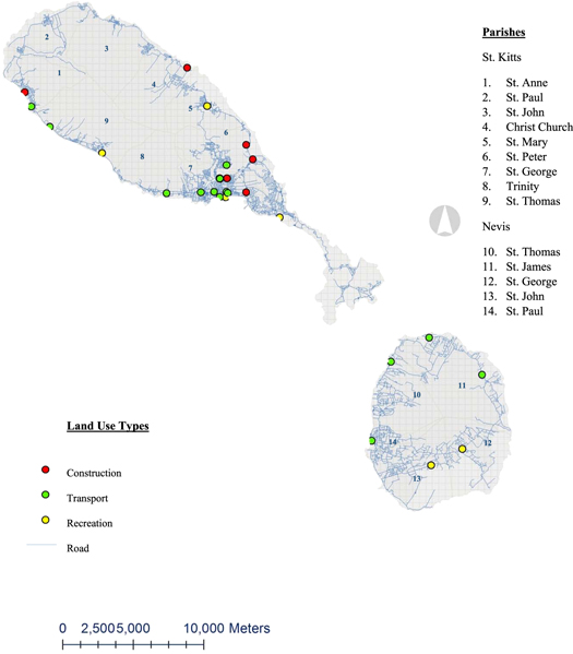
Figure 1. Gridded map of St. Kitts and Nevis showing proposed sampling sites.
Download figure:
Standard image High-resolution imageEnvironmental monitoring
There were twelve (12) 2-week ambient-air monitoring campaigns between early October 2015 and late November 2018. Portable electronic devices were employed for each pollutant of interest: Aeroqual Series 500 for NO2, SO2 and O3, with the appropriate sensors; TSI DustTrak II Handheld Aerosol Monitor—model8532 for PM2.5 and PM10. Moving from Northwest St. Kitts to Southeast Nevis, an average of 3 (1 to 6) sites were monitored per sample day. The devices were temporarily installed at each location between 1 and 1.75 meters from the ground and operated for 15 min to 1 h at a log rate of 60 s between the hours of 6:30 AM and 6:30 PM. We focused on daytime hours as this is the time that the majority of the population tends to initiate, undertake and complete daily outdoor activities related to pollution sources and therefore would be most relevant for public health. Site data inclusion criteria were as follows: (i) minimum duration of each sampling session = 0.25 h; (ii) each site had to be monitored at least twice per sampling campaign; (iii) at least one AM and one PM sample collected per site during each sampling campaign; (iv) at least one dry season and one wet season sample collected per site during each sampling campaign. Background measures at interfaces of cropland and sparsely-populated residential areas were also captured for control purposes.
Spatial land use characteristics (such as the proximity to road, distance from coast, built area, green space, and other land use features within each 500 m × 500 m cell) were noted prior to the sampling campaigns. Additional notes were made during the sampling interval in the event there were unexpected activities taking place at a given site (e.g. closure of major roadways, evidence of a recent fire or initiation of construction projects). Given potential contributions of vehicle exhaust to ambient air pollution concentrations, traffic volumes per hour were also measured concurrently to active sampling. Particular attention was given to (i) certain additional diurnal characteristics (such as non-commuter hours between 8:30 and 11:30 AM; between 1:30 and 4:30 PM; between 6:00 and 7:00 PM and (ii) seasonal intervals (specifically wet season traditionally from May to October and tourist (tour) season from late November to April with a small window in June).
Hourly meteorological data (temperature, humidity, wind direction and incidence of rainfall) for each monitoring session were obtained from local weather stations and a NOAA Weather Radar & Alerts App for Android phones while onsite. Large-scale social activities (e.g. music festivals or street parades) and extreme events (e.g. fires or Sahara Dust plumes) were also noted per their potential to influence air quality.
Analytic methods—data analysis
For descriptive analyses, average and maximum values for each pollutant, site, sampling campaign (n = 12 campaigns), and land use type were presented. To assess co-occurrence of air pollutants, Spearman correlations across pollutant concentrations were evaluated. Differences in pollutant concentrations between locations and sampling times were determined using t-tests and analysis of variance (one-way ANOVA). Tukey tests (multiple comparison procedures) post hoc analysis were used for comparison across sites and across timepoints.
To evaluate predictive factors that explained variability in air pollutant concentrations, linear mixed-effects models were constructed separately for each of the five pollutants using R's lmerTest package. The concentration of the pollutant of interest was the outcome variable. Fixed effects included the other measured ambient air pollutants, land use characteristics (e.g. proximity to road or traffic volume), meteorological features (e.g. temperature or rainfall) and temporal elements (e.g. time of day). Fixed effect covariates were selected for consideration for the final model if (i) statistically significant in preliminary analyses or (ii) if reported to impact pollutant concentrations in previous studies, thereafter retained in final models if they remained statistically significant. Random effects included sampling site (to allow each site to have its own baseline) and timepoint (to account for repeated measures at the same location). Models were constructed separately for untransformed pollutant concentrations and log10-transformed pollutant concentrations. Models were then evaluated using the following goodness-of-fit criteria tests: lower Akaike information criterion (AIC), lower Bayesian information criterion (BIC), higher log-likelihood ratio tests and higher R2.
Analyses were conducted with and without outliers. Potential outliers for NO2, SO2, O3, PM2.5 and PM10 (identified as influential data points exceeding the 75th percentile plus 1.5 times the interquartile range) were replaced with the 95th percentile value of the full distribution of the respective pollutant. R (Studio Version 1.1.463) and SAS 9.4 (SAS Institute Inc.) was employed for all analyses. Significance was set at alpha = 0.05 level; marginally at 0.1.
Results
Pollution—descriptions and associations
The characteristics of the sampling sites are shown in table 1. Across 27 sites, mean NO2, O3, SO2, PM10 and PM2.5 levels were 26.61 ppb (range: 0–306 ppb), 11.94 ppb (0–230 ppb), 27.9 ppb (0–700 ppb), 52.9 μg m−3 (0–10,400 μg m−3) and 29.8 μg m−3 (0–1556 μg m−3), respectively.
Table 1. Land use characteristics of sampling sites in St. Kitts and Nevis.
| Area (m2) | |||||||||||||
|---|---|---|---|---|---|---|---|---|---|---|---|---|---|
| Site rank | Parish | Island | Population | Land use type | Monitor from road (m) | Coast | Water body | Road | Vegetation | Built | SESa | High urban | Tourist activities |
| BAA | Saint George | St. Kitts | 14000 | Transport | 0.2 | 1426.48 | 0.00 | 0.00 | 0.1 | 0.08 | 9 | Yes | No |
| BAH | Saint George | St. Kitts | 14000 | Construction | 6 | 1426.48 | 0.00 | 0.00 | 0.1 | 0.08 | 9 | Yes | No |
| BTT | Saint George | St. Kitts | 14000 | Transport | 0.75 | 271 | 0.00 | 0.12 | 0.02 | 0.11 | 9 | Yes | Yes |
| BTY | Saint Anne | St. Kitts | 3200 | Transport | 5 | 34.49 | 0.02 | 0.00 | 0.09 | 0.07 | 10 | No | No |
| BOU | Christ Church | St. Kitts | 3200 | Construction | 1 | 269.6 | 0.00 | 0.12 | 0.02 | 0.11 | 13 | No | No |
| BIH | Saint Anne | St. Kitts | 14000 | Transport | 1 | 819.73 | 0.00 | 0.00 | 0.25 | 0.00 | 10 | No | No |
| BTL | Saint George | St. Kitts | 2000 | Transport | 5 | 269.99 | 0.00 | 0.00 | 0.17 | 0.08 | 9 | Yes | No |
| CYN | Saint Mary | St. Kitts | 3500 | Recreation | 0.5 | 1323.4 | 0.00 | 0.02 | 0.13 | 0.08 | 11 | Yes | No |
| CFB | Saint George | St. Kitts | 14000 | Transport | 0.5 | 397.63 | 0.00 | 0.03 | 0.1 | 0.11 | 9 | Yes | No |
| CHN | Saint Paul | Nevis | 1800 | Transport | 5 | 20 | 0.01 | 0.00 | 0.08 | 0.06 | 6 | Yes | Yes |
| CTC | Saint Peter | St. Kitts | 3700 | Construction | 7 | 4 | 0.06 | 0.00 | 0.00 | 0.1 | 9 | No | No |
| FRB | Saint George | St. Kitts | 14000 | Recreation | 175 | 20 | 0.07 | 0.01 | 0.03 | 0.02 | 1 | No | Yes |
| GNG | Saint George | Nevis | 2600 | Recreation | 2 | 283.76 | 0.00 | 0.01 | 0.24 | 0.01 | 8 | No | No |
| GOR | Saint George | St. Kitts | 14000 | Construction | 5 | 10 | 0.05 | 0.01 | 0.01 | 0.05 | 1 | Yes | No |
| INS | Saint George | St. Kitts | 14000 | Recreation | 0.25 | 271 | 0.00 | 0.12 | 0.02 | 0.11 | 9 | Yes | Yes |
| JNF | Saint George | St. Kitts | 14000 | Transport | 0.5 | 1058.95 | 0.00 | 0.04 | 0.05 | 0.16 | 9 | Yes | No |
| LFL | Saint George | St. Kitts | 14000 | Construction | 0.5 | 266.45 | 0.15 | 0.00 | 0.02 | 0.01 | 1 | No | No |
| MPR | Saint George | Nevis | 2600 | Recreation | 700 | 2565.78 | 0.00 | 0.01 | 0.16 | 0.08 | 8 | No | Yes |
| NEW | Saint James | Nevis | 1800 | Transport | 1 | 1340 | 0.00 | 0.03 | 0.12 | 0.1 | 2 | No | Yes |
| PZ | Saint George | St. Kitts | 14000 | Recreation | 0.5 | 271 | 0.00 | 0.12 | 0.02 | 0.11 | 9 | Yes | Yes |
| RLB | Saint Peter | St. Kitts | 3700 | Transport | 100 | 5 | 0.05 | 0.01 | 0.01 | 0.06 | 9 | Yes | Yes |
| RSU | Trinity | St. Kitts | 1800 | Transport | 15 | 377.04 | 0.00 | 0.03 | 0.2 | 0.02 | 3 | No | No |
| SBG | Saint Thomas | Nevis | 3000 | Transport | 10 | 15 | 0.02 | 0.06 | 0.08 | 0.01 | 12 | No | Yes |
| SN | Saint Thomas | St. Kitts | 2500 | Recreation | 10 | 11 | 0.02 | 0.04 | 0.06 | 0.01 | 12 | Yes | Yes |
| STJ | Saint James | Nevis | 1800 | Transport | 5 | 1029.45 | 0.00 | 0.01 | 0.21 | 0.03 | 2 | No | No |
| TTS | Saint Anne | St. Kitts | 3200 | Construction | 1.75 | 15 | 0.03 | 0.00 | 0.06 | 0.05 | 10 | Yes | No |
| WAH | Saint George | St. Kitts | 14000 | Transport | 6.00 | 1426.48 | 0.00 | 0.00 | 0.10 | 0.08 | 9 | Yes | No |
aSocioeconomic status ranking based on average resident income in Parish.
Pollutants were generally significantly positively correlated with other. The exception was PM10, which was negatively correlated with all pollutants other than PM2.5 (figure 2). Pollutant levels varied by location. NO2, PM2.5, and PM10 profiles between the islands of St. Kitts and Nevis differed significantly (table 2). Mean concentrations for each pollutant varied significantly by sampling site (p < 0.0001) as shown in figure 3 (data in supplementary table A is available online at stacks.iop.org/ERC/2/041002/mmedia).
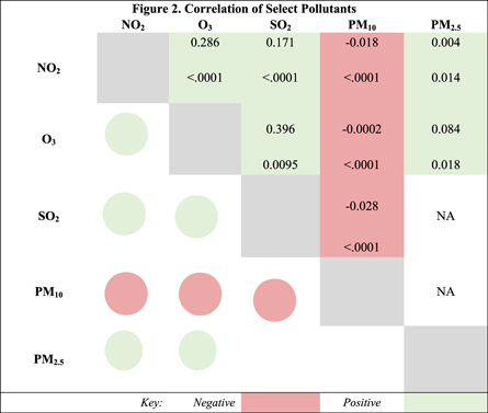
Figure 2. Correlation of Select Pollutants.
Download figure:
Standard image High-resolution imageTable 2. Pollutant concentrations per island across sampling campaigns.
| Pollutant (unit) | St. Kitts | Nevis | |||||||
|---|---|---|---|---|---|---|---|---|---|
| n |  |
max | s | n | |
max | s | p (t-test) | |
| NO2 (ppb) | 12168 | 27 | 306 | 26 | 713 | 23 | 81 | 17 | <.0.0001 |
| O3 (ppb) | 8227 | 12 | 230 | 13 | 666 | 11 | 106 | 13 | 0.0313 |
| SO2 (ppb) | 2475 | 28 | 700 | 51 | NA | ||||
| PM10 (μg m−3) | 7634 | 55 | 10400 | 338 | 528 | 25 | 248 | 28 | <.0.0001 |
| PM2.5 (μg m−3) | 774 | 31 | 1556 | 89 | 130 | 16 | 103 | 17 | <.0.0001 |
n–sample size; -sample mean; s-sample standard deviation.

Figure 3. Ambient air pollutant concentrations by sampling site. Note: Different (combinations of) letters indicate significant differences (p < 0.05) per post-hoc Tukey tests.
Download figure:
Standard image High-resolution imageSites designated as high urban had higher concentrations for all pollutants except for PM2.5 (table 3). Locations that served as venues for tourist activities tended to have lower concentrations of NO2 and SO2 and PM2.5, while PM10 was significantly higher. O3 did not differ according to tourist activity. With respect to land utilization, NO2 and PM2.5 averaged the highest levels at construction sites at 29 ppb (max = 306) and 68.0 μg m−3 (max = 1556), respectively. O3 and PM10 averaged the highest levels at recreational sites: 12.4 ppb (max = 203) and 86 μg m−3 (max = 10,400), respectively. Mean SO2 concentrations were highest at transport sites, averaging 36 ppb (max = 700), while levels around recreational and constructions sites were much lower at 19 ppb and 11 ppb, respectively. All pollutant concentrations varied significantly across specific land use types (p < 0.0001). Differences are illustrated in figure 4. Average background concentrations for NO2, O3, SO2, PM10 and PM2.5 were negligible; 2.4 ppb (0–37 ppb), 2.2 ppb (0–35 ppb), 3.1 ppb (1–7 ppb), 4.4 μg m−3 (0–290 μg m−3) and 4.4 μg m−3 (0–7 μg m−3) respectively.
Table 3. Air pollutant concentrations per additional terrestrial traits and activities.
| NO2 (ppb) | O3 (ppb) | SO2 (ppb) | PM10 (μg m−3) | PM2.5 (μg m−3) | ||||||||||||||||
|---|---|---|---|---|---|---|---|---|---|---|---|---|---|---|---|---|---|---|---|---|
| Traits/Activities | |
max | s | pa | |
max | s | pa | |
max | s | pa | |
max | s | pa | |
max | s | pa |
| Urban | ||||||||||||||||||||
| Low | 22 | 306 | 16 | <0.0001 | 9.7 | 106 | 11 | <0.0001 | 12 | 170 | 23 | <0.0001 | 44 | 2070 | 109 | 0.049 | 35 | 582 | 119 | <0.30 |
| High | 28 | 156 | 27 | 12.4 | 230 | 13 | 30 | 700 | 54 | 54 | 10400 | 352 | 27 | 1556 | 50 | |||||
| Tourist Activities | ||||||||||||||||||||
| Yes | 23 | 189 | 20 | <0.0001 | 12 | 230 | 15 | 0.7000 | 20 | 320 | 32 | <0.0001 | 81 | 10400 | 551 | <0.0001 | 25 | 44 | 44 | 0.0801 |
| No | 28 | 306 | 28 | 12 | 106 | 12 | 31 | 700 | 57 | 37 | 3690 | 100 | 33 | 1556 | 100 | |||||

Figure 4. Pollutant concentrations by specific land use types (construction, recreation and transport): (a) NO2, (b) O3, (c) SO2, (d) PM10, (e) PM2.5. Significance levels per ANOVA tests: *0.05; **0.01; ***0.001; ****<0.001 ns: not significant. Note: Concentration scales for particulate matter graphs (d) and (e) zoomed in thus appearing truncated.
Download figure:
Standard image High-resolution imageTime significantly affected air quality profiles in a number of ways (figure 5). NO2, SO2 and PM10, concentrations tended to be higher in the afternoon. PM10 levels were higher during non-commuter hours. All pollution levels were higher in the wet season with the exception of SO2. Some pollutant concentrations were significantly different in the tourist (tour) season compared to other time periods. Levels were significantly higher for all pollutants except for PM2.5, which was notably lower. Table 4 presents additional temporal differences: campaign, year, month, day of the week. Smoothed time-trend curves are shown in figure 6.
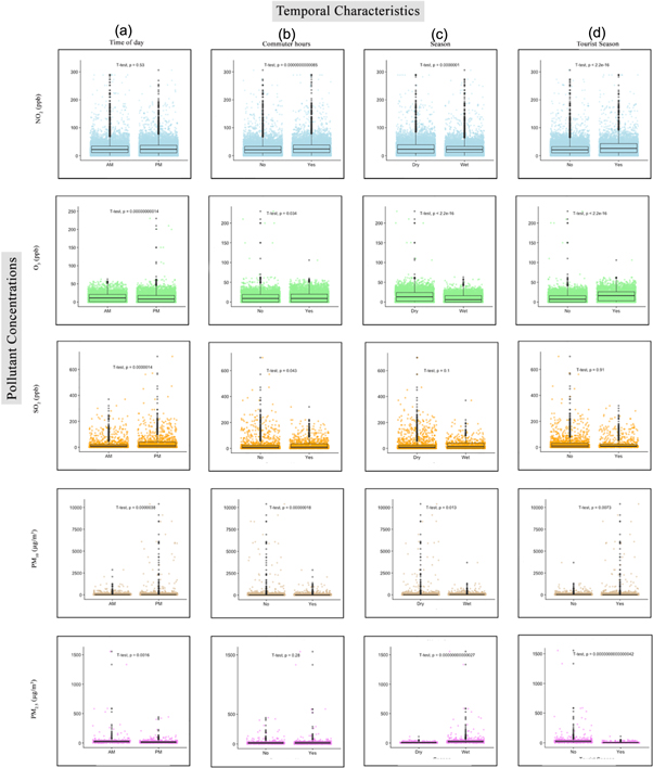
Figure 5. Air pollutant concentrations per various temporal characteristics: (a) time of day, (b) commuter hours, (c) meteorological season, (d) tourist (tour) season.
Download figure:
Standard image High-resolution imageTable 4. Temporal characteristics and differences across air pollutants.
| Temporal | NO2 (ppb) | O3 (ppb) | SO2 (ppb) | PM10 (μg m−3) | PM2.5 (μg m−3) | |||||||||||||||
|---|---|---|---|---|---|---|---|---|---|---|---|---|---|---|---|---|---|---|---|---|
| characteristics | |
max | s | group | |
max | s | group | |
max | s | group | |
max | s | group | |
max | s | group |
| Campaign/Timepoint | ||||||||||||||||||||
| 1sta | 25.0 | 15 | 182 | cde | 8.2 | 7.9 | 28 | e | 13 | 19 | 122 | b | 1.1 | 1.4 | 5 | b | ||||
| 2nd | 42.0 | 23 | 125 | a | 9.3 | 10 | 106 | e | 11 | 33 | 302 | b | 3.5 | 5.1 | 38 | b | ||||
| 3rd | 16.0 | 15 | 105 | f | 12.3 | 11.9 | 62 | d | 48 | 113 | 2070 | b | 10.4 | 15.5 | 108 | b | ||||
| 4th | 18.0 | 18 | 97 | f | 12.6 | 11.9 | 39 | d | 41 | 55 | 922 | b | 20 | 4.8 | 36 | ab | ||||
| 5th | 26.0 | 28 | 273 | cd | 10.1 | 9.7 | 58 | e | 42 | 73 | 1262 | b | 49 | 143.3 | 1556 | a | ||||
| 6th | 24.0 | 26 | 306 | de | 4.6 | 7.4 | 50 | f | 27.2 | 46.1 | 240 | a | 41 | 123 | 3690 | b | 38.7 | 51.7 | 442 | a |
| 7th | 28.0 | 40 | 289 | bc | 16.3 | 12.8 | 44 | c | 28 | 46.6 | 320 | a | 31 | 182 | 2870 | b | ||||
| 8th | 44.0 | 32 | 252 | a | 26.1 | 13.9 | 57 | a | 12.1 | 11.6 | 44 | b | 107 | 746 | 10400 | a | ||||
| 9th | 23.0 | 22 | 273 | e | 13.9 | 10.7 | 45 | cd | 6.6 | 4.8 | 16 | b | 28 | 68 | 922 | b | ||||
| 10th | 19.0 | 16 | 73 | ef | 11.8 | 9.7 | 63 | de | 33.5 | 40.3 | 370 | a | 154 | 684 | 6910 | a | ||||
| 11th | 30.0 | 25 | 254 | b | 21.9 | 8.6 | 35 | b | 30.7 | 65.9 | 700 | a | 55 | 51 | 257 | b | ||||
| 12tha | 22.0 | 18 | 113 | e | 12.3 | 21.2 | 230 | d | 33 | 14 | 79 | b | ||||||||
| p (F-test) | p < 0.0001 | p < 0.0001 | p < 0.0001 | p < 0.0001 | p < 0.0001 | |||||||||||||||
| Day | ||||||||||||||||||||
| Sundaya | 28 | 16 | 129 | ab | 9.1 | 7.1 | 30 | b | 40 | 39 | 318 | b | 22 | 2.3 | 30 | ab | ||||
| Monday | 27 | 22 | 273 | ab | 13.2 | 13 | 62 | b | 36.5 | 67.1 | 700 | a | 21 | 31 | 411 | b | 22 | 42.7 | 312 | ab |
| Tuesday | 22 | 26 | 252 | b | 10.3 | 11.5 | 58 | b | 13.4 | 31 | 240 | c | 32 | 90 | 2870 | b | 14 | 12.2 | 108 | b |
| Wednesday | 27 | 26 | 273 | ab | 11.2 | 15.4 | 230 | a | 26.9 | 53.7 | 470 | b | 112 | 633 | 10400 | a | 27 | 49.8 | 442 | ab |
| Thursday | 30 | 29 | 306 | a | 12 | 11.6 | 63 | b | 32.6 | 43 | 370 | ab | 40 | 64 | 1262 | b | 43 | 139.6 | 1556 | a |
| Friday | 29 | 30 | 289 | ab | 15.1 | 13.8 | 57 | b | 24.5 | 40.8 | 320 | b | 39 | 112 | 2070 | b | 39 | 91.6 | 582 | ab |
| Saturdaya | 24 | 15 | 129 | ab | 10 | 9.6 | 39 | b | 5.2 | 6.4 | 23 | c | 41 | 164 | 2870 | b | 19 | 4.8 | 35 | ab |
| p (F-test) | p < 0.0001 | p < 0.0001 | p < 0.0001 | p < 0.0001 | p < 0.0001 | |||||||||||||||
| Month | ||||||||||||||||||||
| January | 43 | 31 | 252 | a | 20.7 | 15 | 106 | a | 28 | 46.6 | 320 | a | 92.4 | 686 | 10400 | a | 4 | 5.9 | 38 | c |
| April | 17 | 16 | 105 | d | 12.3 | 11.9 | 62 | b | 9.5 | 7.9 | 28 | b | 45 | 98 | 2070 | b | 12.5 | 14.5 | 108 | c |
| May | 23 | 22 | 273 | c | 14.5 | 10.7 | 45 | b | 12.6 | 12.2 | 44 | b | 28.2 | 71 | 922 | b | ||||
| June | 23 | 21 | 273 | c | 9.8 | 8.4 | 63 | c | 6.1 | 4.9 | 15 | b | 31.8 | 37 | 345 | b | 24.6 | 12.9 | 62 | bc |
| July | 25 | 31 | 306 | bc | 8.1 | 9.8 | 58 | c | 7 | 4.7 | 16 | b | 64.2 | 280 | 6910 | ab | 52 | 133.3 | 1556 | a |
| August | 25 | 20 | 139 | bc | 3.8 | 6.3 | 50 | d | 31.6 | 50 | 778 | b | 42.8 | 71 | 442 | ab | ||||
| October | 27 | 20 | 254 | b | 13.5 | 10.5 | 35 | b | 33.5 | 40.3 | 370 | a | 51.5 | 50 | 257 | b | 1.1 | 1.4 | 5 | c |
| Novembera | 24 | 26 | 289 | c | 13.6 | 19 | 230 | b | 29.8 | 61.9 | 700 | a | 30.6 | 178 | 2870 | b | ||||
| p (F-test) | p < 0.0001 | p < 0.0001 | p < 0.0001 | p < 0.0001 | p < 0.012 | |||||||||||||||
| Year | ||||||||||||||||||||
| 1-Y2015 | 25 | 15 | 182 | b | 8.2 | 7.9 | 28 | c | 9.7 | 18 | 147 | b | 1.6 | 1.5 | 5 | b | ||||
| 2-Y2016 | 24 | 26 | 306 | bc | 9.1 | 10.6 | 106 | c | 27 | 46 | 240 | a | 40.2 | 112 | 3690 | b | 31.1 | 84.7 | 1556 | a |
| 3-Y2017 | 34 | 29 | 273 | a | 22.1 | 13 | 63 | a | 26 | 39 | 370 | a | 77 | 510 | 10400 | a | ||||
| 4-Y2018 | 22 | 18 | 113 | c | 12.3 | 21.2 | 230 | b | 31 | 66 | 700 | a | 33.2 | 14 | 79 | b | ||||
| p (F-test) | p < 0.0001 | p < 0.0001 | 0.008 | p < 0.0001 | 0.0012 | |||||||||||||||
Different letters in group columns indicate significant differences (p < 0.05) per post-hoc Tukey tests. aSummary does not include data from all monitoring sites.
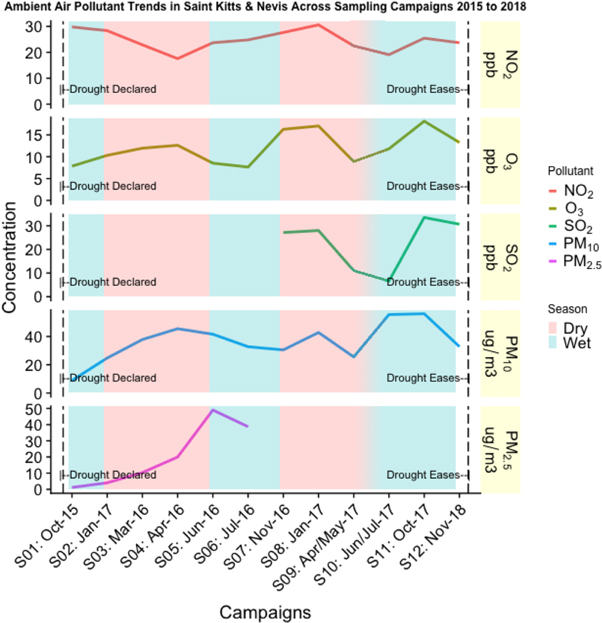
Figure 6. Smoothed time curve ambient air pollutant trends in St. Kitts—Nevis across sampling campaigns 2015 to 2018, intervals of drought and meteorological season included.
Download figure:
Standard image High-resolution image
Per an interim tour of sampling locations in June 2016, it was observed that construction projects were initiated in 26 of the 27 sites selected for sampling. The contribution of these activities could not be parsed despite attempts to log and analyze site and district-specific events. The parishes with the most construction projects proximate to sampling sites were St. Peter (n = 10), St. Anne (n = 12), St. Mary (13), St. George in St. Kitts (24) and St. Thomas in St. Kitts (26), all designated as urban except for the last.
Onsite researchers observed remnant plumes of Sahara Dust on July 6, 10 and 11 of 2016; the PM10 concentrations on these three days averaged approximately 25.0 μg m−3 (0–169 μg m−3).
Meteorology
Across all sampling days the mean temperature was 28 °C (σ = 1.6; range of 25 to 28) while maximum temperatures averaged 31 °C (σ = 1.6; range of 27 to 34). Rain averaged <0.1 mm per sampling day, with 89% of days without precipitation. Wind speeds were generally lower than 15 knots/h (17.3 mph) varying in on a daily basis. Relative humidity ranged from 63 to 90% with a mean of 73%.
Traffic volume and other potential sources
Estimated traffic volumes ranged widely from 0 to 852 vehicular crossings, averaging 144 per hour (σ = 138). Mean hourly crossings were 70% higher at transport sites (182) than both construction (101) and recreation (107) sites, a significant difference (p < 0.0001).
Modelling
A total of 20 models were constructed. The linear mixed models for each pollutant generally included a number of fixed effects including weather, land use and time (table 5) although some were more parsimonious, relying on a single covariate. R2 ranged substantially, with the lowest value for untransformed PM10 (7.66%) and the highest for log10-transformed PM2.5 (70%). The other best-fit criteria supported log-transformed pollutant-specific models. Tourist season and specific months, more than any other factors, contributed most to variability in pollutant concentrations. Other explanatory variables such as drought, parish, and precipitation were occasionally important factors included in final models. Timepoint did not consistently improve the fit of most pollutant-specific model. (Additional data in supplementary table B).
Table 5. Pollutant concentration linear mixed effect models; random effect variables preselected; explanatory fixed variables significant at α = 0.05.
| Pollutant | Response form | Model | Random effects | AIC | BIC | Log likelihood | R2 (%) |
|---|---|---|---|---|---|---|---|
| NO2 | NO2 | 0.55*O3 + 23.03*Month(January) + 10.72*Month(July) − 14.43*LUT(Recreation) + 26.13* Parish(Saint Mary) + 8.29* Parish(Saint James) | Site | 3107.49 | 3123.07 | −1549.75 | 35.12 |
| NO2 | 0.57*O3 + 14.28*LUT(Recreation) | Site + Timepoint | 3069.70 | 3182.64 | −1505.85 | 36.13 | |
| Log10NO2 | 0.77*ß0 + 0.51*Month(January) + 0.17*Log10O3 + 0.26*Month(October) + 0.24*Month(July) + 0.24*Month(November) − 0.21* LUT(Recreation) + 0.27* Month(August) + 0.35*Parish(Saint Mary) | Site | 159.43 | 174.61 | −75.72 | 32.87 | |
| Log10NO2 | 0.54*Month(January) + 0.19*Log10O3 + 0.19*Month(October) + 0.21*Month(July) + 0.27*Month(November) − 0.20* LUT(Recreation) + 0.25* Month(August) + 0.37*Parish(Saint Mary) | Site + Timepoint | 102.67 | 212.67 | −22.34 | 32.38 | |
| O3 | O3 | −9724.46*ß0 + 0.19*NO2–0.017*Proximity(Road) + 8.44*TOURSeason + 4.83*Year + 6.77*Season(wet) − 5.07*Month(July) − 7.62*Month(August) | Site | 2620.04 | 2760.24 | −1274.02 | 39.14 |
| O3 | 0.17*NO2 | Site + Timepoint | 2607.14 | 2751.23 | −1266.57 | 53.19 | |
| Log10O3 | 0.24*TOURSeason + 0.45*Log10NO2–0.0005*Traffic − 0.26*Month(July) − 0.50*Month(August) | Site | 420.69 | 549.65 | −176.35 | 31.60 | |
| Log10O3 | 0.42* Log10NO2 + 0.0005*Traffic | Site + Timepoint | 412.54 | 549.09 | −170.27 | 51.70 | |
| SO2 | SO2 | 4.80*Temp + 1.01*O3 | Site | 1190.79 | 1255.47 | −572.39 | 35.91 |
| SO2 | 4.80*Temp + 1.01*O3 | Site + Timepoint | 1192.79 | 1260.28 | −572.39 | 35.91 | |
| Log10SO2 | 0.39* Log10NO2 + 0.32*Rain + 0.55* Log10O3 + 0.014*RelHum − 0.0025*RWindDir | Site | 141.81 | 205.54 | −47.91 | 51.90 | |
| Log10SO2 | 0.39* Log10NO2 + 0.32*Rain + 0.55* Log10O3 + 0.014*RelHum − 0.0025*RWindDir | Site + Timepoint | 143.81 | 210.31 | −47.91 | 51.90 | |
| PM10 | PM10 | 182.79*Parish(Saint Thomas ∣ St. Kitts) | Site | 3872.19 | 3957.22 | −1913.10 | 7.66 |
| PM10 | 182.79*Parish(Saint Thomas ∣ St. Kitts) | Site + Timepoint | 3874.19 | 3962.92 | −1913.10 | 7.66 | |
| Log10PM10 | 2.28*ß0–0.46*TOURSeason − 0.013*RelHum + 0.0009*RWindDir | Site | 405.58 | 490.38 | −179.79 | 30.26 | |
| Log10PM10 | 2.16*ß0–0.47*TOURSeason − 0.011*RelHum + 0.0008*RWindDir | Site + Timepoint | 407.58 | 496.07 | −179.79 | 31.91 | |
| PM2.5 | PM2.5 | 140.28*Parish(Saint Thomas ∣ Nevis) − 48.83* LUT(Transport) | Site | 929.30 | 988.75 | −440.65 | 34.01 |
| PM2.5 | 140.28*Parish(Saint Thomas ∣ Nevis)− 48.83* LUT(Transport) | Site + Timepoint | 931.30 | 993.23 | −440.65 | 34.01 | |
| Log10PM2.5 | −0.64*TOURSeason + 0.63*Drought − 0.0014*RelHum | Site | 107.60 | 167.05 | −29.80 | 70.14 | |
| Log10PM2.5 | −0.64*TOURSeason + 0.63*Drought − 0.0014*RelHum | Site + Timepoint | 109.60 | 171.53 | -29.80 | 70.46 |
LUT—Land Use Type; RWindDir—direction relative to nearest road (clockwise in 15 degree increments); TOURSeason—Tourist Season; Temp—Temperature; RelHum—Relative Humidity; Drought—dry conditions per 2015; additional data in supplementary table B.
Discussion and conclusion
This air sampling study provided new information on a range of pollutants and their determinants in this understudied area of the Eastern Caribbean. It is the first of its kind in the nation of St. Kitts and Nevis, finding land use type, tourism season and to some lesser extent, drought, to be unique factors contributing to air pollutant concentration variability. Results offer insight for future exposure and health studies as well as context for policy makers regarding ambient air quality.
The higher concentrations of PM2.5 and NO2 at constructions sites could respectively be attributed to the movement and grading of building materials [16, 18] as well as the relative contributions of energy being used during building activities [59]. SO2 levels likely peaked at transport sites due to the emissions profiles of various larger vehicles (e.g. passenger buses, taxi vans and diesel trucks) in spaces specifically configured for transport [60, 61], showing no difference across tour seasons as many of the sample locales would operate similarly year-round.
Previous studies showed urban areas tend to have more diminished air quality [62–64]. This increased risk of hazard has been framed as an environmental justice issue [65, 66] especially for those socioeconomically disadvantaged [63, 64, 67, 68]. In this investigation, most pollutant concentrations were elevated in high urban areas to varying degrees possibly owing to the selective action of the urban heat island (UHI) effect [69–71], short-term atmospheric conditions such as humidity and temperature [72] or long-term weather events such as drought [73]. Loss of significance due to urban levels (low versus high) was likely the result of mixed land use and configurations within varying urban form [74, 75].
The findings do suggest a general increase in ambient air pollution during tourist season as observed in other parts of the world [11, 76, 77].
Some social events, typically well-attended by SKN residents and visitors, did coincide with sampling schedules, most of them annual recreational affairs that are associated with increased traffic volumes as well as outdoor cook stove use [78] (e.g. St. Kitts' music festival, Nevis' Culturama and the St. Kitts and Nevis carnival celebrations held in June, August and December, respectively). That said, levels were significantly lower in areas where tourist activities take place, possibly as a result of transport between tourist sites being the major pollution. SN, an open-air recreational site undergoing renovations and known for cook stove use, was an exception with notably higher PM10 and PM2.5 levels, consistent with previous studies focused on the contributions of construction activities [16, 79] and smoke [80–82] to particulate matter concentrations.
With the exception of NO2 which is likely bimodal in its AM-PM concentration distribution, pollutant levels trended higher in the later hours of the day (after 12 PM) aligning with previous studies as it relates to traffic pollution [83–85]. Diurnal significance would however diminish in constructed models.
The moderate drought conditions that persisted from late-2014 to mid-2017 likely depressed the difference between seasons for levels of particulate matter. PM10 concentrations may have been lower in the designated wet season if not for the dry spell, as precipitation has been associated with suppression of particulate and some gaseous air pollutants [86–88]. The effect of rainfall deficits on air pollution levels aligns with observations and predictions of previous studies that indicate some association between climate change effects such as drought and air quality [89–92].
Ports and populated coastal areas with heavy ship traffic can be exposed to particulate emissions from marine vessels [93]. However, the convoy of terrestrial transport vehicles (e.g. buses and taxis) that would congregate at such sites (e.g. PZ) were likely key contributors to inland traffic pollution as previously observed [94]. Alternatively, various atmospheric factors could have impacted PM10 [13], which seems evident in cases where traffic did not significantly factor into concentration models.
Average Sahara Dust PM10 concentration was significantly lower than the study mean of 49.6 μg m−3. This could be the result of low deposition, as the Sahara Air Layer (SAL) is typically bounded between altitudes 1.5 and 3.7 km above sea level [95], well beyond the highest point in SKN (Mount Liamuiga) at 1.16 km. However, three days of data might not serve as sufficiently informative.
The constructed multivariate models had notably variable prediction capacities, only one with R2 higher than 70%. Their usefulness could be constrained for a number of reasons including but not limited to the absence of unknown yet critical explanatory variables, the complexity of land use activities within specific land utilization types of interest, the uncaptured residual effect of other environmental events such as heavy precipitations between campaigns, or simply limited data across spatiotemporal scales. The notable poor performance of untransformed PM10 models (R2 less than 10%) is additionally likely due to the high impact of the SN site (Saint Thomas in St. Kitts). Logarithmic transformation of air pollutant concentrations, an approach conveniently and effectively applied in previous air quality studies [96, 97], potentially overcame some of aforementioned constraints.
It is important to note that all final analyses presented herein included potential outliers. The presence of these higher, possibly overly influential values, did impact the significance of certain covariates. Applying the outlier replacement procedure outlined in the methods did yield slightly stronger correlations among all pollutants, a few notably different covariates in constructed models for SO2, PM10 and PM2.5, and slightly higher R2 values for models for non-gaseous pollutants. However, we resolved that opting to remove this data risks sacrificing critical site-specific information and generating interpretations based on truncated data arguably more misleading than interpretations using the original data with potential outliers. Maximum values (e.g. 10.4 mg m−3 for PM10 and 1.6 mgm−3 for PM2.5) are short-term peaks and should not be construed as representing the long-term air quality of the region.
There are a few limitations to the study. First, not all pollutants were measured across all sites, on all days, and across multiple monitoring periods due to issues with site access and functional monitors. As such, some temporal summaries, namely descriptive statistics, across certain days, months and campaigns could not be generated, most notably for SO2 and PM2.5. On average, five out of the seven weekdays, generally Monday to Friday, were evaluated for pollution at each site. Overall, the analysis of these pollutants still have utility with regard to the profile of local air quality even if constrained by missing-ness per the aims of determining associations with land use features.
Second, in terms of design, the air quality estimates herein were based on short-term ambient air monitoring with handheld devices and no fixed monitoring sites with which to complement or compare. However, the portable devices employed in this study have been found to be sufficiently and reliably correlated with other established ambient air surveillance equipment [98–100]. Third, researchers did not attempt 24-h surveillance. Nevertheless, the 6:30 AM to 6:30 PM interval (a) was sufficient to evaluate pollution per land use type as well as other sources, (b) most comfortably facilitated the most efficient use of the portable monitors, each having limited batteries requiring daily recharge (c) helped to ensure the safety of onsite study personnel operating sampling devices and (d) is most relevant to etiology as this is the time that the majority of the population would tend to initiate, undertake and complete daily outdoor activities. Moreover, background concentrations suggest that the 12 hours not accounted for could have been negligible or at least very low.
Fourth, in reality, air pollution is dynamic and subject to migrations across local boundaries [101, 102]. As such, constraining air quality estimates spatially, based on land use across such small landmasses with mixed and changing characteristics might not be ideal. That said, the stratified and purposeful random sampling method ensured increased spatial coverage across research sites. Additionally, ad hoc adjustments for social activities, construction projects and extreme events generally did little to alter the significance in differences between categories in various analysis.
Finally, some districts (such as St. Mary, Trinity and St. Thomas, Nevis) were only represented by a single site while others contained many (e.g. St. George, St. Kitts). This might have resulted in parish districts being determined as more significant predictors of pollutions estimates than land use type. However, as this could not be reconciled without removing key sample sites, it seemed prudent to proceed with analyses that involve the complex mixture of land use types that are characteristic of SKN and many other Eastern Caribbean parish districts. While beyond the scope of this investigation, future studies should consider the heterogeneity within districts.
There are however notable strengths to this investigation as well. Given absence of spatial datasets for this understudied region, the creative use of multiple data resources, specifically the combination of GIS, local records and onsite characterizations, was vital to reducing misclassification of land use types and so category-specific concentration estimates. Additionally, investigations such as this one underscore the importance of micro-scale studies in developing tropical locales when engaging air pollution dynamics in smaller landmasses. Furthermore, this study evaluated multiple pollutants per their sources, interactions and impacting factors, both addressing a dearth of air pollution research in small island developing states and contributing to the wider global literature regarding spatiotemporal aspects of ambient air quality. Lastly, this probe of five target pollutants, which are considered to be criteria pollutants by the USEPA and important per WHO guidelines, can facilitate in the future, better quantification of health risk factors, offer critical information to epidemiological researchers and inform policymakers designing interventions, particularly in the EC region.
Overall, this study contributes to evidence of air pollution in small developing nations and provides some of the first systematic, albeit limited, monitoring in the Eastern Caribbean where surveillance systems are not yet established. Additionally, results offer insight into the change in air quality as a result of urban development features and at least one profound extreme weather event, specifically drought. Significance of land use types was generally limited to bivariate analysis, yet specific land use features, time and meteorology proved important factors in relation to air pollution levels. Further investigation is warranted with respect to pollutant spatiotemporal dynamics in the Eastern Caribbean setting, especially during intervals that would provide opportunity to compare air quality during non-drought periods to the pollutant concentrations recorded in this study. Estimating exposure and disease burdens relative to the pollution levels and accordingly risk categories is currently being explored in research carried out by some authors of this paper in order to determine the degree to which the air quality in this understudied region indeed might have etiological relevance.
Acknowledgments
The authors would like to acknowledge the financial support of the Yale Institute for Biospeheric Science (YIBS) in preliminary fieldwork source of funding for your research; the technical support of the Bell Research Group; the administrators of the Yale School of Public Health (YSPH), including but not limited to Dr Krystal Pollitt, Dr Robert Dubrow and Dr Brian Leaderer for their contributions to the development of the manuscript; administrators and students of the Clarence Fitzroy Bryant College (CFBC) in St. Kitts, especially students of the Environmental Science and Chemistry Departments who contributed to fieldwork; the SKN Ministries of Planning & Sustainable Development for the use of local land use records; the St. Kitts and Nevis Meteorological Offices for provision of weather data; other local partners; my relatives, friends and partners in SKN; the journal reviewers and editors of this manuscript.