
Using Object Detection on Social Media Images for Urban Bicycle Infrastructure Planning: A Case Study of Dresden

 ,
,  , , , and
Abstract
:1. Introduction
2. Related Work
- Use of stationary sensors to count passing bicycles,
- Analysis of public surveillance videos through object detection,
- GPS-tracking through devices used by cyclists,
- Tracking of GPS devices directly mounted on bicycles.
3. Method
3.1. Dataset
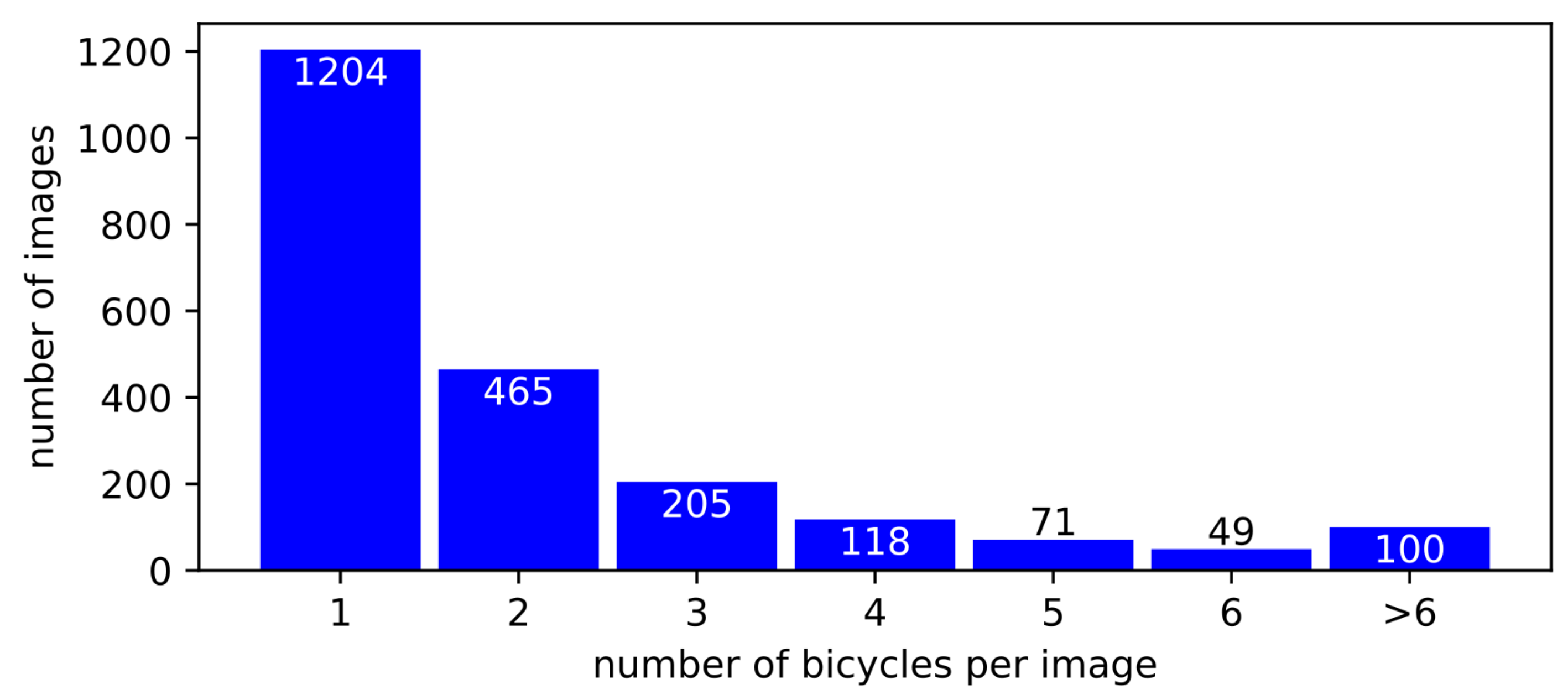
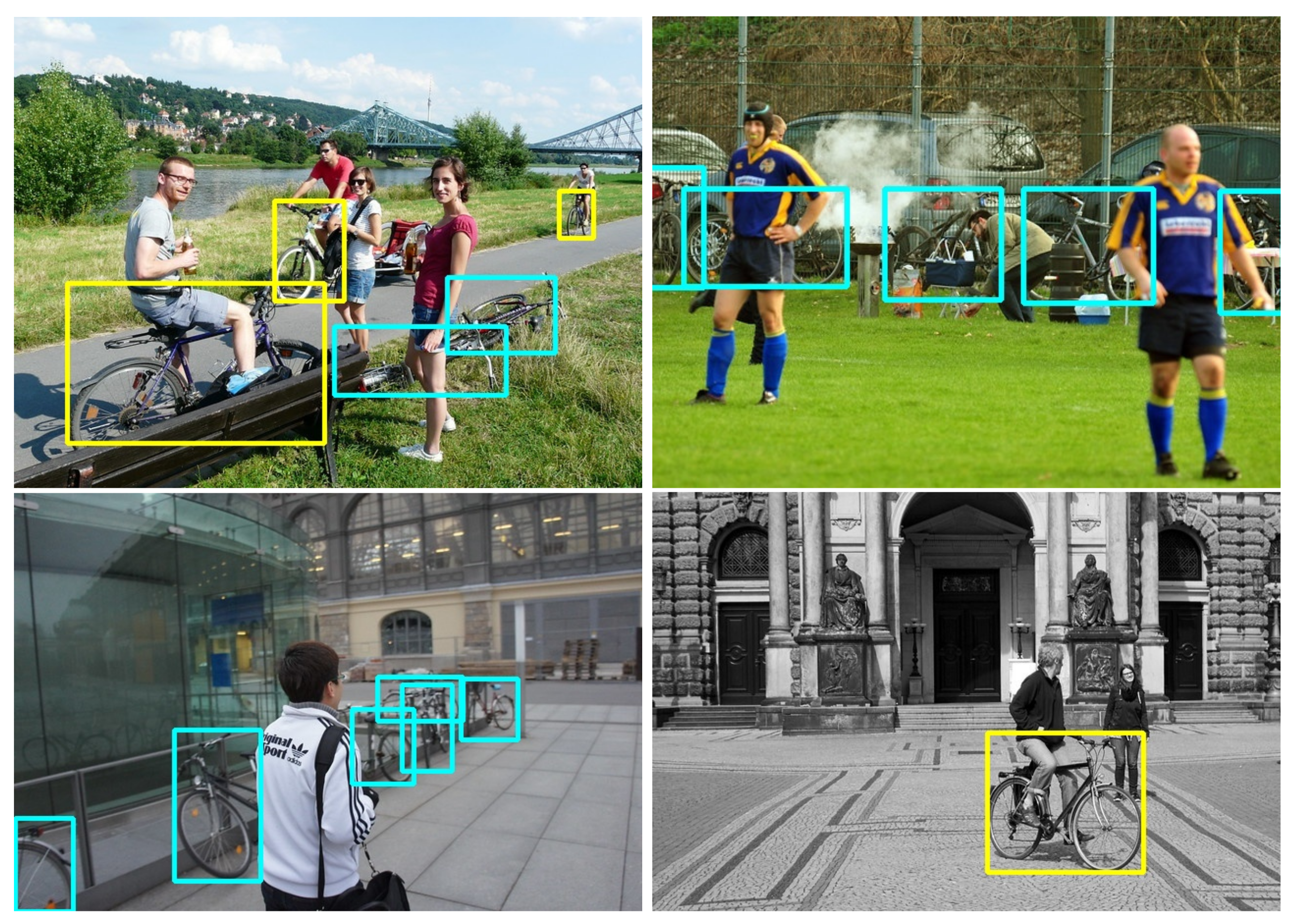
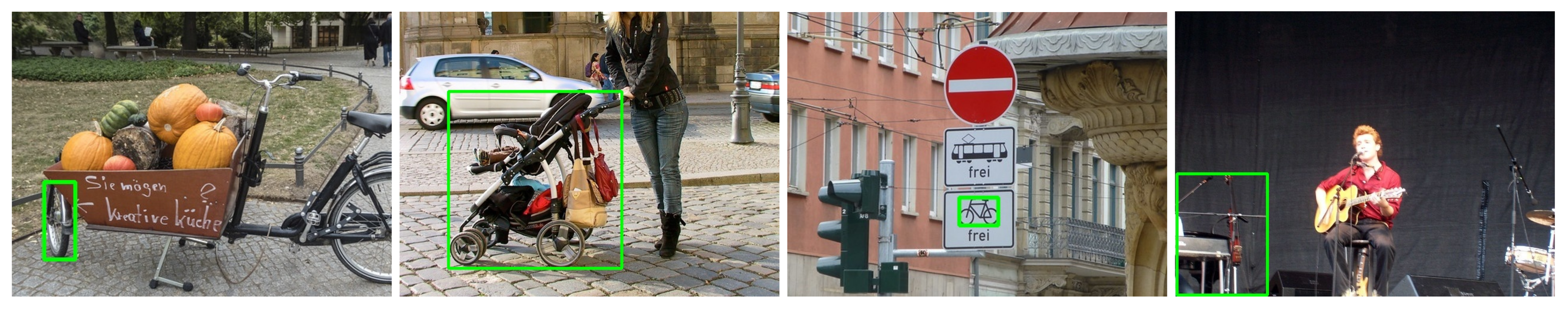
3.1.1. Bicycle Annotations
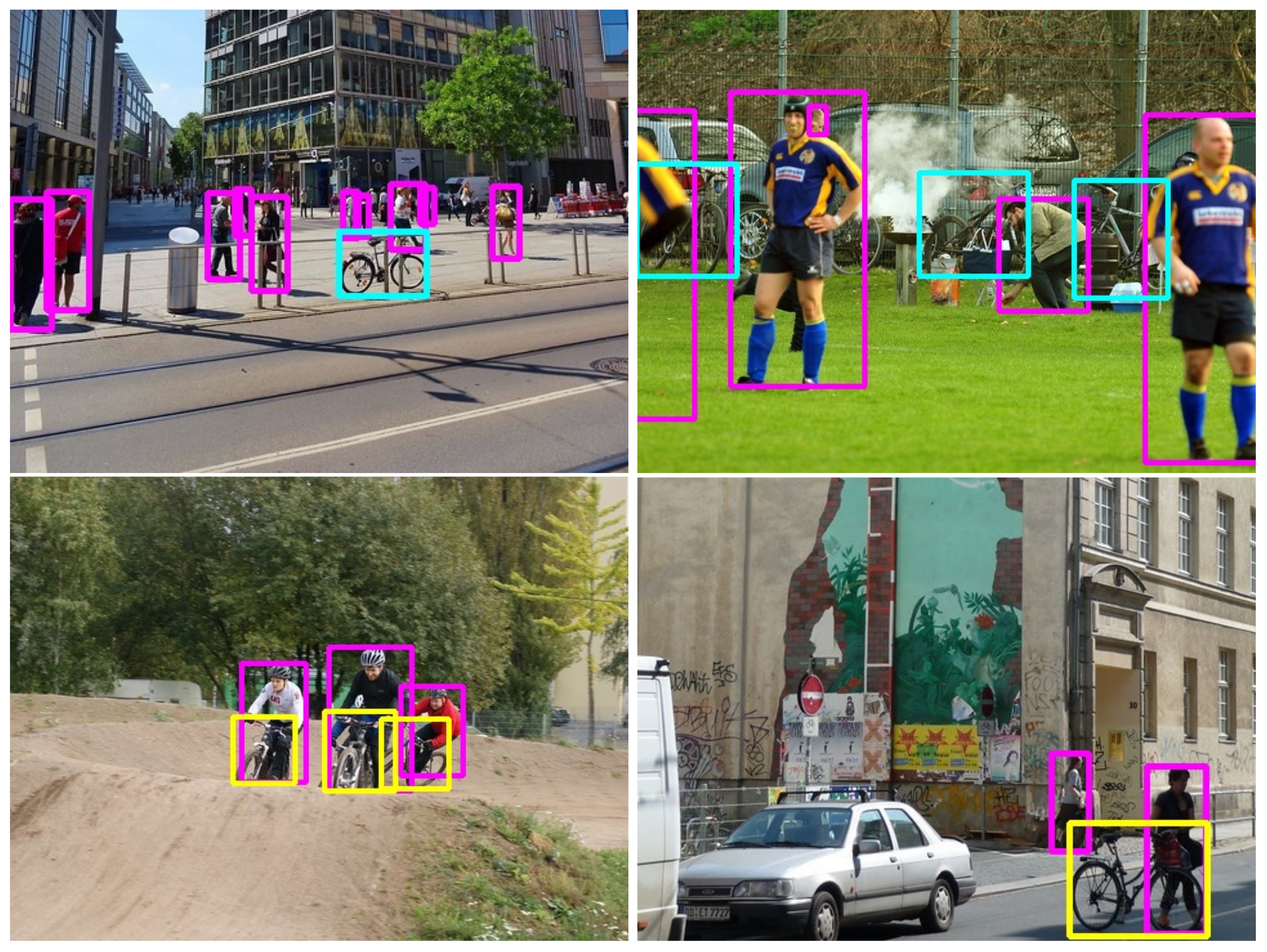
3.2. Object Detection
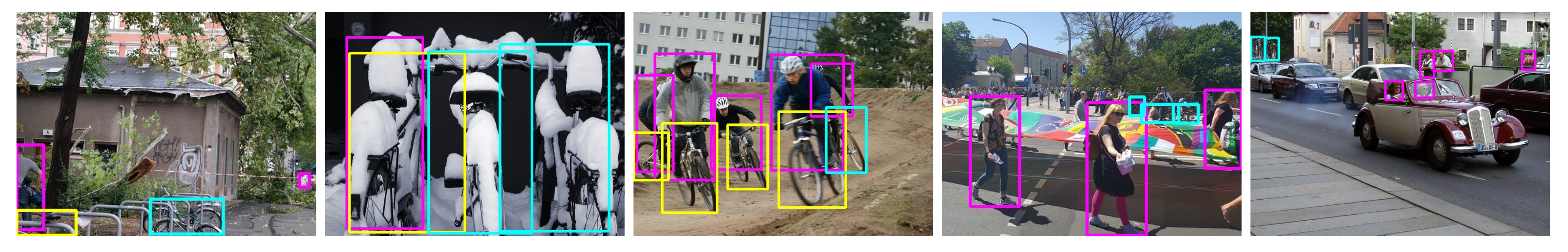
3.2.1. Moving Bicycles
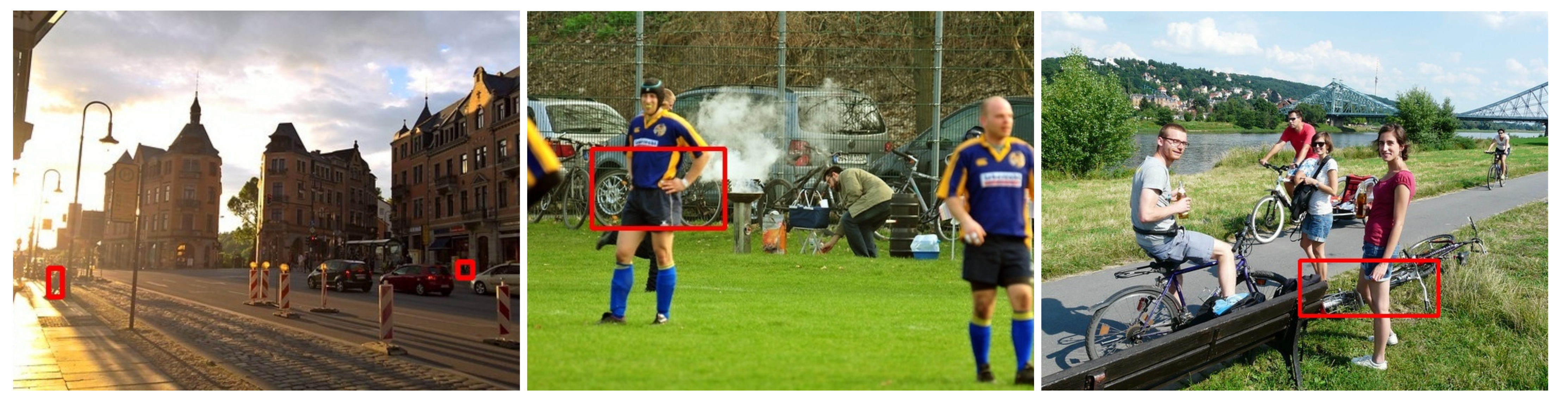
3.3. Evaluating Detections
3.4. Determining Thresholds
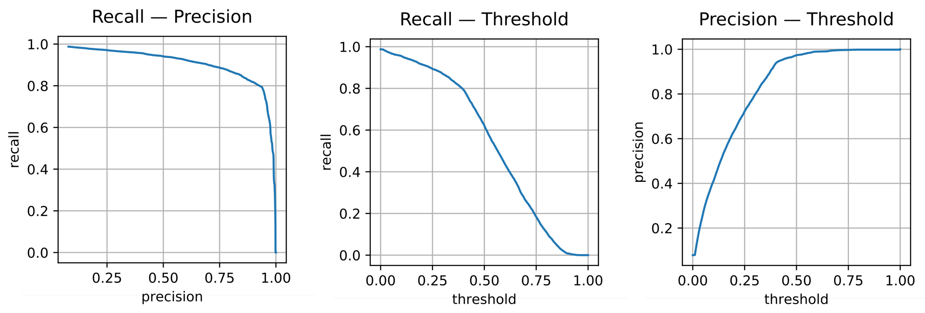
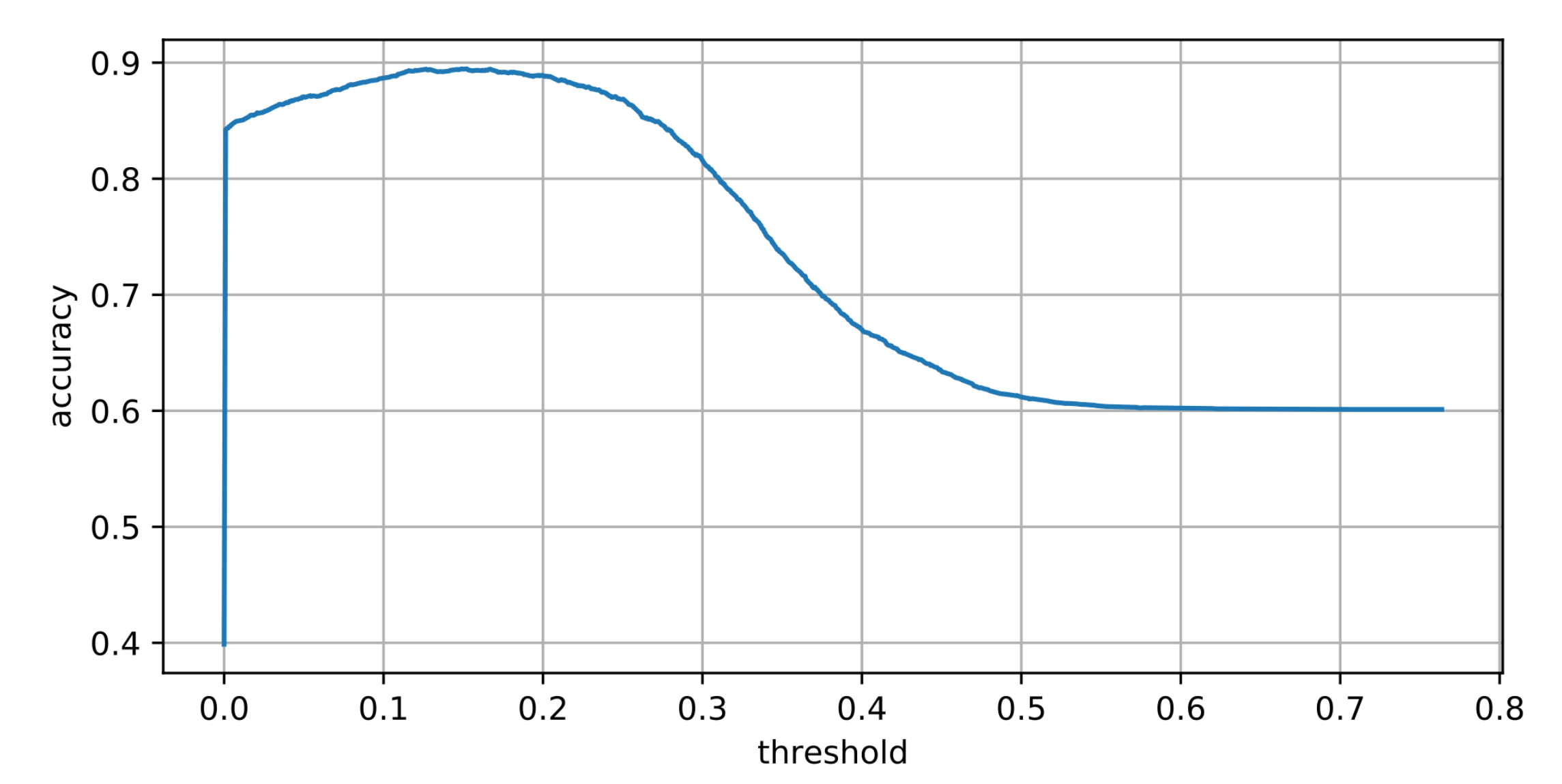
3.4.1. Confidence Threshold
3.4.2. Person Assignment Threshold
4. Bicycle Detection Results
4.1. Detection Accuracy
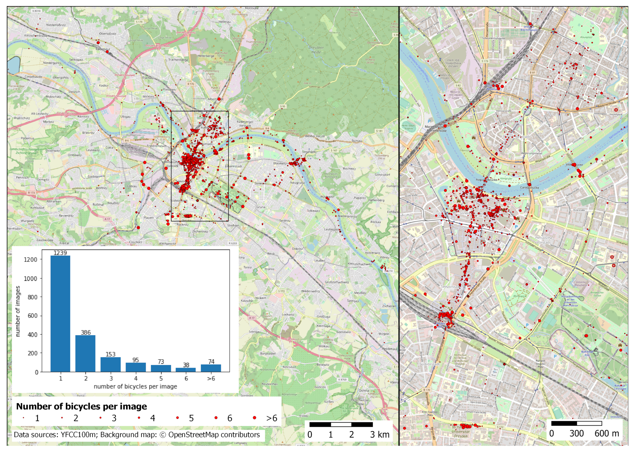
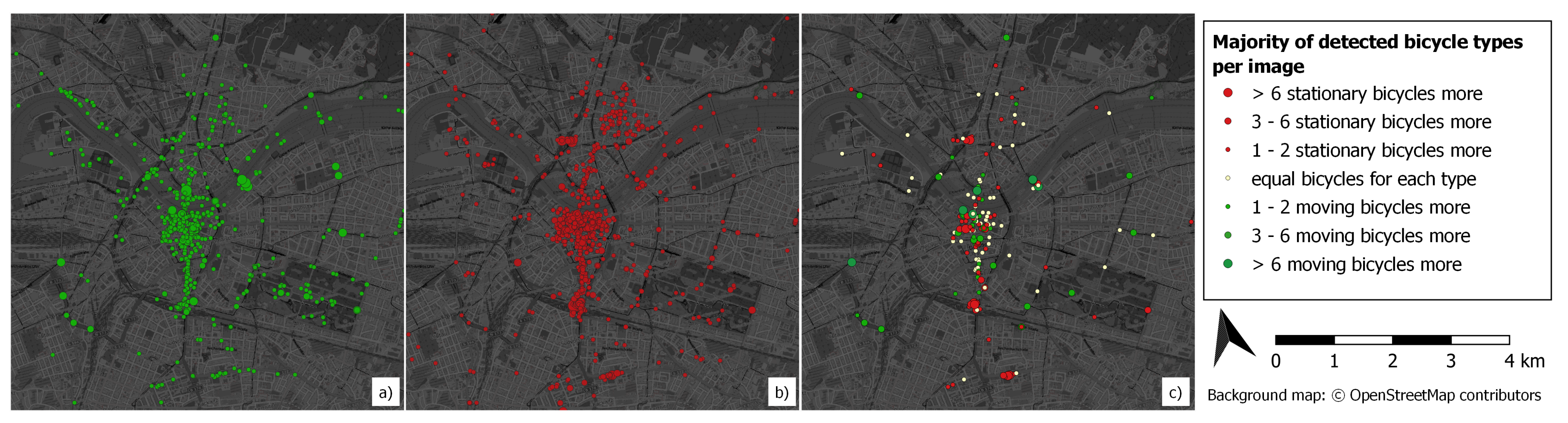
4.2. Spatial Distribution of Recognized Bicycles
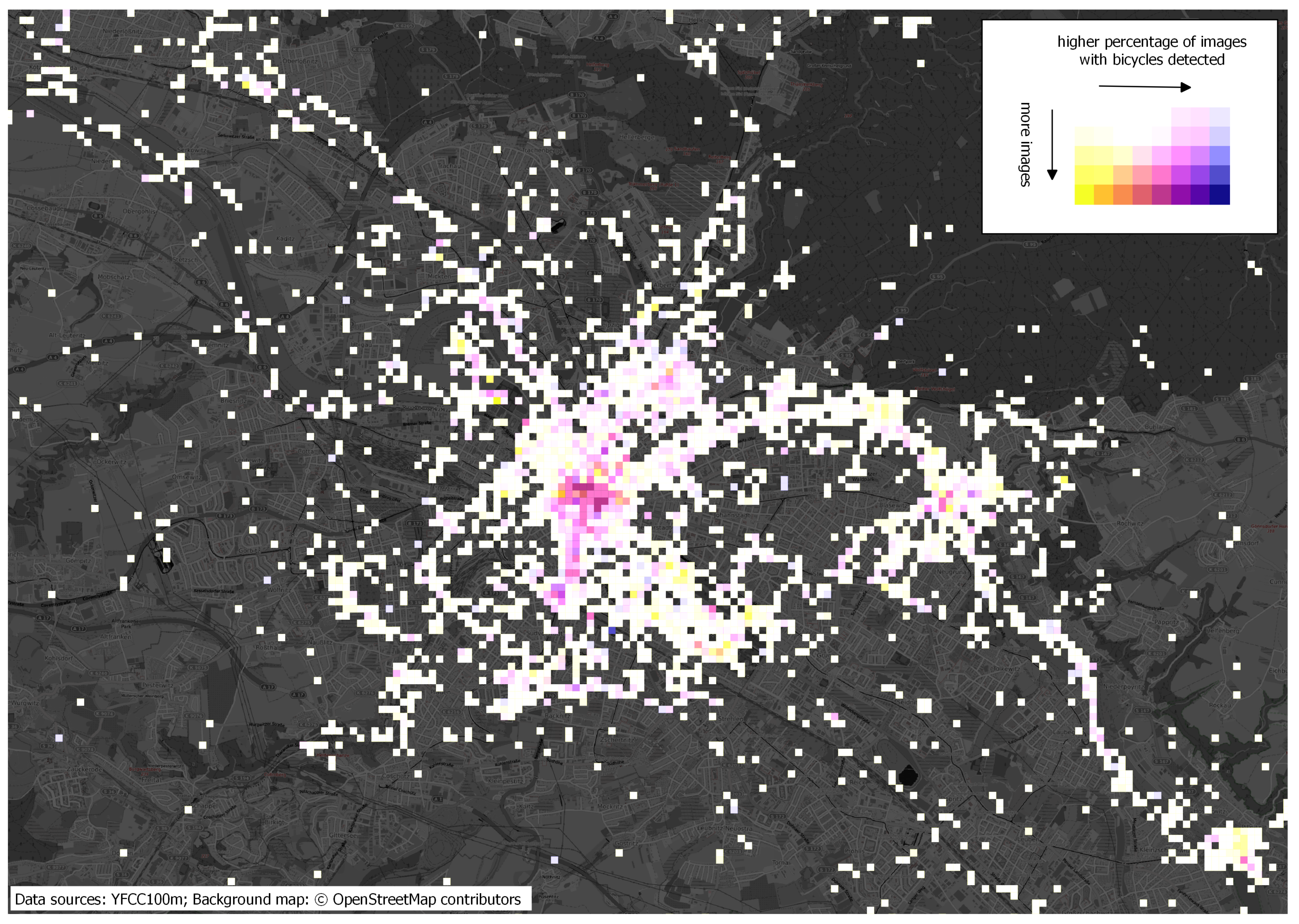
4.3. Density of Images with Detected Bicycles
- The number of images in the YFCC100m Dresden subset,
- The number of bicycles detected on images from the subset,
- The number of stationary bicycles detected,
- The number of moving bicycles detected,
- The number of images containing at least one bicycle,
- The number of images containing at least one stationary bicycle,
- The number of images containing at least one moving bicycle.
4.4. Comparison with Other Datasets
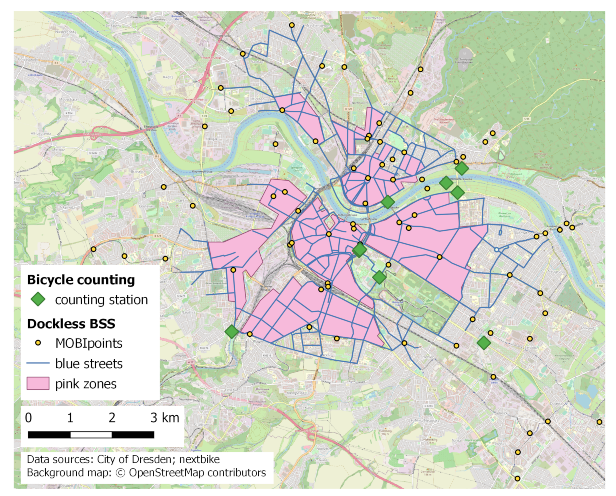
- The positions of the stationary bicycle counting sensors installed by the city administration of Dresden.
- The defined bicycle return areas and a sample of positions of parked bicycles from the bicycle sharing system MOBI, obtained at different points in time throughout a week in September 2021.
4.4.1. Bicycle Counting Stations
4.4.2. Bicycle Sharing Systems
5. Case Study
5.1. Number of Parked Bicycles vs. Percentage of Photos Containing Parked Bicycles
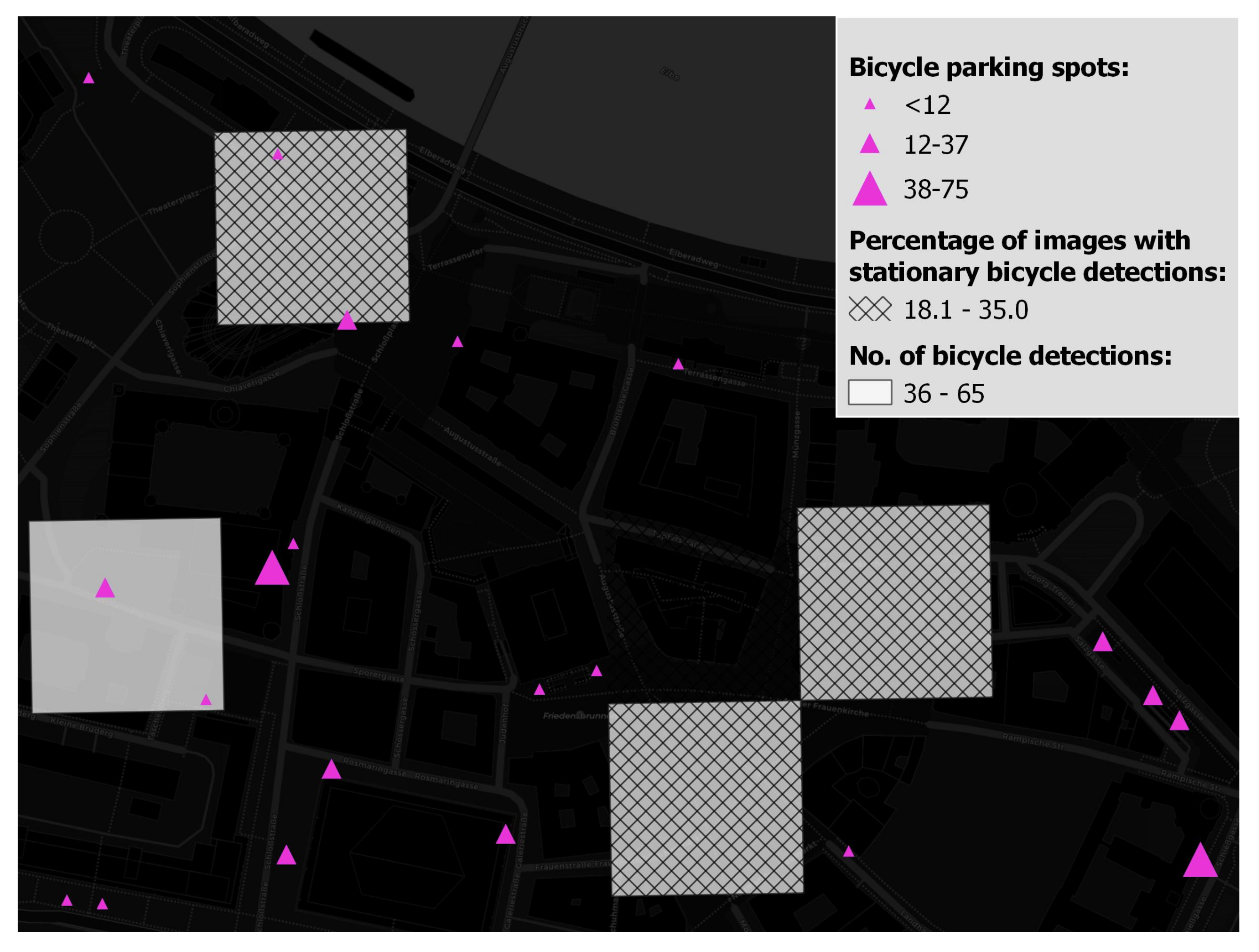
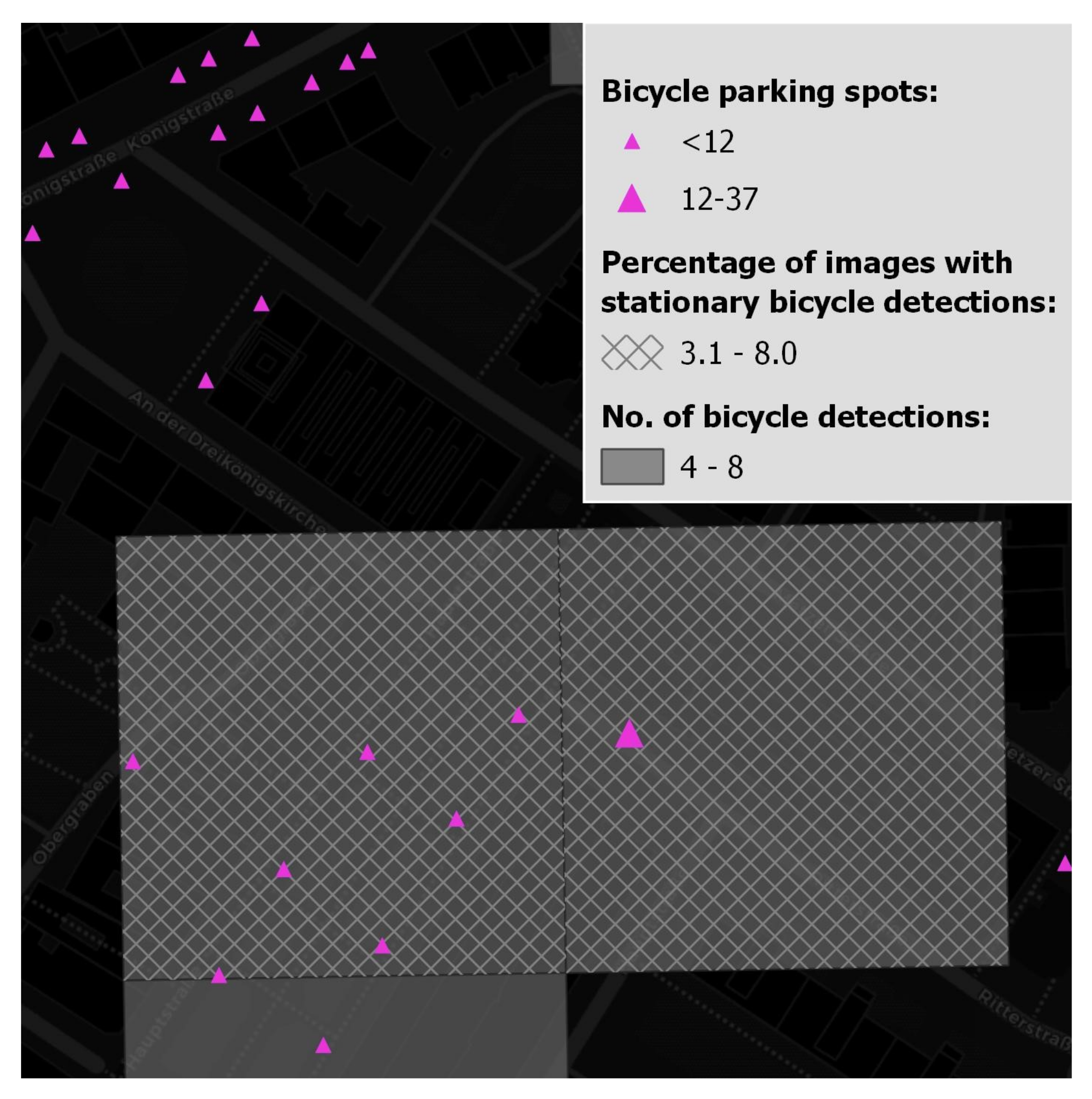
5.2. Number of Parked Bicycles vs. Percentage of Photos Containing Parked Bicycles vs. Number of Available Parking Spots
5.3. Summary of Results
6. Discussion
6.1. Object Detection on Social Media Data as an Additional Data Source for Obtaining Bicycle-Related Information in Urban Areas
6.2. Relevance of Time in Our Approach
6.3. Influence of Bicycle Detection Errors and Potential Improvements
7. Conclusions
Author Contributions
Funding
Data Availability Statement
Conflicts of Interest
References
- Sumantran, V.; Fine, C.; Gonsalvez, D. Faster, Smarter, Greener: The Future of the Car and Urban Mobility; The MIT Press: Cambridge, MA, USA, 2017. [Google Scholar] [CrossRef]
- Qiu, L.Y.; He, L.Y. Bike Sharing and the Economy, the Environment, and Health-Related Externalities. Sustainability 2018, 10, 1145. [Google Scholar] [CrossRef] [Green Version]
- Pucher, J.; Buehler, R. Making Cycling Irresistible: Lessons from The Netherlands, Denmark and Germany. Transp. Rev. 2008, 28, 495–528. [Google Scholar] [CrossRef]
- Froehlich, J.; Neumann, J.; Oliver, N. Sensing and Predicting the Pulse of the City through Shared Bicycling. In Proceedings of the 21st International Jont Conference on Artifical Intelligence, Pasadena, CA, USA, 14–17 July 2009; pp. 1420–1426. [Google Scholar]
- Zhou, X. Understanding Spatiotemporal Patterns of Biking Behavior by Analyzing Massive Bike Sharing Data in Chicago. PLoS ONE 2015, 10, e0137922. [Google Scholar] [CrossRef] [PubMed]
- Corcoran, J.; Li, T.; Rohde, D.; Charles-Edwards, E.; Mateo-Babiano, D. Spatio-temporal patterns of a Public Bicycle Sharing Program: The effect of weather and calendar events. J. Transp. Geogr. 2014, 41, 292–305. [Google Scholar] [CrossRef]
- Etienne, C.; Latifa, O. Model-Based Count Series Clustering for Bike Sharing System Usage Mining: A Case Study with the VéLib’ System of Paris. ACM Trans. Intell. Syst. Technol. 2014, 5, 1–21. [Google Scholar] [CrossRef]
- Korpilo, S.; Virtanen, T.; Lehvävirta, S. Smartphone GPS tracking—Inexpensive and efficient data collection on recreational movement. Landsc. Urban Plan. 2017, 157, 608–617. [Google Scholar] [CrossRef] [Green Version]
- Reades, J.; Calabrese, F.; Sevtsuk, A.; Ratti, C. Cellular Census: Explorations in Urban Data Collection. IEEE Pervasive Comput. 2007, 6, 30–38. [Google Scholar] [CrossRef] [Green Version]
- Huber, S.; Lissner, S.; Schnabel, A.; Lindemann, P.; Friedl, J. Modelling bicycle route choice in German cities using open data, MNL and the bikeSim web-app. In Proceedings of the 2021 7th International Conference on Models and Technologies for Intelligent Transportation Systems (MT-ITS), Heraklion, Greece, 16–17 June 2021. [Google Scholar] [CrossRef]
- Chen, C.; Anderson, J.C.; Wang, H.; Wang, Y.; Vogt, R.; Hernandez, S. How bicycle level of traffic stress correlate with reported cyclist accidents injury severities: A geospatial and mixed logit analysis. Accid. Anal. Prev. 2017, 108, 234–244. [Google Scholar] [CrossRef]
- Götschi, T.; Garrard, J.; Giles-Corti, B. Cycling as a Part of Daily Life: A Review of Health Perspectives. Transp. Rev. 2016, 36, 45–71. [Google Scholar] [CrossRef] [Green Version]
- Buehler, R. Determinants of transport mode choice: A comparison of Germany and the USA. J. Transp. Geogr. 2011, 19, 644–657. [Google Scholar] [CrossRef]
- Scott, D.M.; Lu, W.; Brown, M.J. Route choice of bike share users: Leveraging GPS data to derive choice sets. J. Transp. Geogr. 2021, 90, 102903. [Google Scholar] [CrossRef]
- Hoogendoorn, S.; Daamen, W. Bicycle Headway Modeling and Its Applications. Transp. Res. Rec. 2016, 2587, 34–40. [Google Scholar] [CrossRef] [Green Version]
- Pogodzinska, S.; Kiec, M.; D’Agostino, C. Bicycle Traffic Volume Estimation Based on GPS Data. Transp. Res. Procedia 2020, 45, 874–881. [Google Scholar] [CrossRef]
- Gehrke, S.R.; Reardon, T.G. Direct demand modelling approach to forecast cycling activity for a proposed bike facility. Transp. Plan. Technol. 2021, 44, 1–15. [Google Scholar] [CrossRef]
- Beitel, D.; McNee, S.; Miranda-Moreno, L.F. Quality Measure of Short-Duration Bicycle Counts. Transp. Res. Rec. 2017, 2644, 64–71. [Google Scholar] [CrossRef]
- Turner, S.; Lasley, P. Quality Counts for Pedestrians and Bicyclists: Quality Assurance Procedures for Nonmotorized Traffic Count Data. Transp. Res. Rec. 2013, 2339, 57–67. [Google Scholar] [CrossRef]
- Hankey, S.; Lu, T.; Mondschein, A.; Buehler, R. Spatial models of active travel in small communities: Merging the goals of traffic monitoring and direct-demand modeling. J. Transp. Health 2017, 7, 149–159. [Google Scholar] [CrossRef]
- Gupte, S.; Masoud, O.; Martin, R.; Papanikolopoulos, N. Detection and classification of vehicles. IEEE Trans. Intell. Transp. Syst. 2002, 3, 37–47. [Google Scholar] [CrossRef] [Green Version]
- Ghosh, A.; Sabuj, M.S.; Sonet, H.H.; Shatabda, S.; Farid, D.M. An Adaptive Video-based Vehicle Detection, Classification, Counting, and Speed-measurement System for Real-time Traffic Data Collection. In Proceedings of the 2019 IEEE Region 10 Symposium (TENSYMP), Kolkata, India, 7–9 June 2019; pp. 541–546. [Google Scholar] [CrossRef]
- Gillis, D.; Gautama, S.; Van Gheluwe, C.; Semanjski, I.; Lopez, A.J.; Lauwers, D. Measuring Delays for Bicycles at Signalized Intersections Using Smartphone GPS Tracking Data. ISPRS Int. J. Geo-Inf. 2020, 9, 174. [Google Scholar] [CrossRef] [Green Version]
- Chen, Z.; van Lierop, D.; Ettema, D. Dockless bike-sharing systems: What are the implications? Transp. Rev. 2020, 40, 333–353. [Google Scholar] [CrossRef]
- Ma, X.; Ji, Y.; Yuan, Y.; Van Oort, N.; Jin, Y.; Hoogendoorn, S. A comparison in travel patterns and determinants of user demand between docked and dockless bike-sharing systems using multi-sourced data. Transp. Res. Part A Policy Pract. 2020, 139, 148–173. [Google Scholar] [CrossRef]
- Basiri, A.; Haklay, M.; Foody, G.; Mooney, P. Crowdsourced geospatial data quality: Challenges and future directions. Int. J. Geogr. Inf. Sci. 2019, 33, 1588–1593. [Google Scholar] [CrossRef] [Green Version]
- Wang, L. Planning for cycling in a growing megacity: Exploring planners’ perceptions and shared values. Cities 2020, 106, 102857. [Google Scholar] [CrossRef]
- Weng, J.; Bäumer, T.; Müller, P. Bike-Sharing Systems as Integral Components of Inner-City Mobility Concepts: An Analysis of the Intended User Behaviour of Potential and Actual Bike-Sharing Users. In Innovations for Metropolitan Areas: Intelligent Solutions for Mobility, Logistics and Infrastructure Designed for Citizens; Planing, P., Müller, P., Dehdari, P., Bäumer, T., Eds.; Springer: Berlin/Heidelberg, Germany, 2020; pp. 121–132. [Google Scholar] [CrossRef]
- Zhu, Z.; Blanke, U.; Calatroni, A.; Tröster, G. Human Activity Recognition Using Social Media Data. In Proceedings of the 12th International Conference on Mobile and Ubiquitous Multimedia, Luleå, Sweden, 2–5 December 2013. [Google Scholar] [CrossRef]
- Stock, K. Mining location from social media: A systematic review. Comput. Environ. Urban Syst. 2018, 71, 209–240. [Google Scholar] [CrossRef]
- Middleton, S.E.; Kordopatis-Zilos, G.; Papadopoulos, S.; Kompatsiaris, Y. Location Extraction from Social Media: Geoparsing, Location Disambiguation, and Geotagging. ACM Trans. Inf. Syst. 2018, 36, 1–27. [Google Scholar] [CrossRef] [Green Version]
- Gong, J.; Li, R.; Yao, H.; Kang, X.; Li, S. Recognizing Human Daily Activity Using Social Media Sensors and Deep Learning. Int. J. Environ. Res. Public Health 2019, 16, 3955. [Google Scholar] [CrossRef] [Green Version]
- Cao, R.; Tu, W.; Yang, C.; Li, Q.; Liu, J.; Zhu, J.; Zhang, Q.; Li, Q.; Qiu, G. Deep learning-based remote and social sensing data fusion for urban region function recognition. ISPRS J. Photogramm. Remote Sens. 2020, 163, 82–97. [Google Scholar] [CrossRef]
- Thomee, B.; Shamma, D.A.; Friedland, G.; Elizalde, B.; Ni, K.; Poland, D.; Borth, D.; Li, L.J. YFCC100M: The new data in multimedia research. Commun. ACM 2016, 59, 64–73. [Google Scholar] [CrossRef]
- Tan, M.; Pang, R.; Le, Q.V. Efficientdet: Scalable and efficient object detection. In Proceedings of the IEEE/CVF Conference on Computer Vision and Pattern Recognition, Seattle, WA, USA, 16–18 June 2020; pp. 10781–10790. [Google Scholar]
- Redmon, J.; Farhadi, A. Yolov3: An incremental improvement. arXiv 2018, arXiv:1804.02767. [Google Scholar]
- Du, X.; Lin, T.Y.; Jin, P.; Ghiasi, G.; Tan, M.; Cui, Y.; Le, Q.V.; Song, X. SpineNet: Learning scale-permuted backbone for recognition and localization. In Proceedings of the IEEE/CVF Conference on Computer Vision and Pattern Recognition, Seattle, WA, USA, 16–18 June 2020; pp. 11592–11601. [Google Scholar]
- He, K.; Gkioxari, G.; Dollár, P.; Girshick, R. Mask r-cnn. In Proceedings of the IEEE International Conference on Computer Vision, Venice, Italy, 22–29 October 2017; pp. 2961–2969. [Google Scholar]
- Lin, T.Y.; Goyal, P.; Girshick, R.; He, K.; Dollár, P. Focal loss for dense object detection. In Proceedings of the IEEE International Conference on Computer Vision, Venice, Italy, 22–29 October 2017; pp. 2980–2988. [Google Scholar]
- Lin, T.Y.; Maire, M.; Belongie, S.; Hays, J.; Perona, P.; Ramanan, D.; Dollár, P.; Zitnick, C.L. Microsoft coco: Common objects in context. In European Conference on Computer Vision; Springer: Berlin/Heidelberg, Germany, 2014; pp. 740–755. [Google Scholar]
- Zoph, B.; Cubuk, E.D.; Ghiasi, G.; Lin, T.Y.; Shlens, J.; Le, Q.V. Learning data augmentation strategies for object detection. In European Conference on Computer Vision; Springer: Berlin/Heidelberg, Germany, 2020; pp. 566–583. [Google Scholar]
- Kuhn, H.W. The Hungarian method for the assignment problem. Nav. Res. Logist. Q. 1955, 2, 83–97. [Google Scholar] [CrossRef] [Green Version]
- Landeshauptstadt Dresden, S.u.T. Dauerzählstellen für den Radverkehr. Available online: http://www.dresden.de/media/pdf/Strassenbau/Dauerzaehlstellen_Stadtplan.pdf (accessed on 5 August 2021).
- Jenks, G.F. The data model concept in statistical mapping. Int. Yearb. Cartogr. 1967, 7, 186–190. [Google Scholar]
- Jiang, B.; Ma, D.; Yin, J.; Sandberg, M. Spatial Distribution of City Tweets and Their Densities. Geogr. Anal. 2016, 48, 337–351. [Google Scholar] [CrossRef] [Green Version]
- Bahadori, M.S.; Gonçalves, A.B.; Moura, F. A Systematic Review of Station Location Techniques for Bicycle-Sharing Systems Planning and Operation. ISPRS Int. J. Geo-Inf. 2021, 10, 554. [Google Scholar] [CrossRef]
- Telefonaktiebolaget LM Ericsson Ericsson Mobility Visualizer. Available online: https://www.ericsson.com/en/mobility-report/mobility-visualizer?f=1&ft=1&r=1&t=8&s=1&u=1&y=2014,2021&c=1 (accessed on 14 September 2021).
- Domínguez, D.R.; Díaz Redondo, R.P.; Vilas, A.F.; Khalifa, M.B. Sensing the city with Instagram: Clustering geolocated data for outlier detection. Expert Syst. Appl. 2017, 78, 319–333. [Google Scholar] [CrossRef]
- Gunter, U.; Önder, I. An Exploratory Analysis of Geotagged Photos From Instagram for Residents of and Visitors to Vienna. J. Hosp. Tour. Res. 2021, 45, 373–398. [Google Scholar] [CrossRef]
- Beigi, G.; Shu, K.; Zhang, Y.; Liu, H. Securing Social Media User Data: An Adversarial Approach. In Proceedings of the 29th on Hypertext and Social Media, Baltimore, MD, USA, 9–12 July 2018; pp. 165–173. [Google Scholar] [CrossRef]
- Dunkel, A.; Löchner, M.; Burghardt, D. Privacy-Aware Visualization of Volunteered Geographic Information (VGI) to Analyze Spatial Activity: A Benchmark Implementation. ISPRS Int. J. Geo-Inf. 2020, 9, 607. [Google Scholar] [CrossRef]
- Löchner, M.; Fathi, R.; Schmid, D.; Dunkel, A.; Burghardt, D.; Fiedrich, F.; Koch, S. Case Study on Privacy-Aware Social Media Data Processing in Disaster Management. ISPRS Int. J. Geo-Inf. 2020, 9, 709. [Google Scholar] [CrossRef]
- Martí, P.; Serrano-Estrada, L.; Nolasco-Cirugeda, A. Social Media data: Challenges, opportunities and limitations in urban studies. Comput. Environ. Urban Syst. 2019, 74, 161–174. [Google Scholar] [CrossRef]
- Alivand, M.; Hochmair, H.H. Spatiotemporal analysis of photo contribution patterns to Panoramio and Flickr. Cartogr. Geogr. Inf. Sci. 2017, 44, 170–184. [Google Scholar] [CrossRef]
- McKenzie, G.; Janowicz, K.; Gao, S.; Yang, J.A.; Hu, Y. POI Pulse: A Multi-granular, Semantic Signature–Based Information Observatory for the Interactive Visualization of Big Geosocial Data. Cartographica 2015, 50, 71–85. [Google Scholar] [CrossRef]
- Nordback, K.; Marshall, W.E.; Janson, B.N.; Stolz, E. Estimating Annual Average Daily Bicyclists: Error and Accuracy. Transp. Res. Rec. 2013, 2339, 90–97. [Google Scholar] [CrossRef]
- Rashidi, T.H.; Abbasi, A.; Maghrebi, M.; Hasan, S.; Waller, T.S. Exploring the capacity of social media data for modelling travel behaviour: Opportunities and challenges. Transp. Res. Part C Emerg. Technol. 2017, 75, 197–211. [Google Scholar] [CrossRef]
- Resch, B.; Usländer, F.; Havas, C. Combining machine-learning topic models and spatiotemporal analysis of social media data for disaster footprint and damage assessment. Cartogr. Geogr. Inf. Sci. 2018, 45, 362–376. [Google Scholar] [CrossRef] [Green Version]
- Girshick, R.; Donahue, J.; Darrell, T.; Malik, J. Rich feature hierarchies for accurate object detection and semantic segmentation. In Proceedings of the IEEE Conference on Computer Vision and Pattern Recognition, Columbus, OH, USA, 23–28 June 2014; pp. 580–587. [Google Scholar]
- Reinders, C.; Ackermann, H.; Yang, M.Y.; Rosenhahn, B. Object recognition from very few training examples for enhancing bicycle maps. In Proceedings of the 2018 IEEE Intelligent Vehicles Symposium (IV), Suzhou, China, 26–30 June 2018; pp. 1–8. [Google Scholar]
- Reinders, C.; Ackermann, H.; Yang, M.Y.; Rosenhahn, B. Learning convolutional neural networks for object detection with very little training data. In Multimodal Scene Understanding; Elsevier: Amsterdam, The Netherlands, 2019; pp. 65–100. [Google Scholar]
- Krizhevsky, A.; Sutskever, I.; Hinton, G.E. Imagenet classification with deep convolutional neural networks. Adv. Neural Inf. Process. Syst. 2012, 25, 1097–1105. [Google Scholar] [CrossRef]
- Zhou, B.; Lapedriza, A.; Khosla, A.; Oliva, A.; Torralba, A. Places: A 10 million Image Database for Scene Recognition. IEEE TRansactions Pattern Anal. Mach. Intell. 2017, 40, 1452–1464. [Google Scholar] [CrossRef] [Green Version]
- Kluger, F.; Reinders, C.; Raetz, K.; Schelske, P.; Wandt, B.; Ackermann, H.; Rosenhahn, B. Region-based cycle-consistent data augmentation for object detection. In Proceedings of the 2018 IEEE International Conference on Big Data (Big Data), Seattle, WA, USA, 10–13 December 2018; pp. 5205–5211. [Google Scholar]
- Dunkel, A.; Andrienko, G.; Andrienko, N.; Burghardt, D.; Hauthal, E.; Purves, R. A conceptual framework for studying collective reactions to events in location-based social media. Int. J. Geogr. Inf. Sci. 2019, 33, 780–804. [Google Scholar] [CrossRef]
- Hauthal, E.; Burghardt, D. Mapping Space-Related Emotions out of User-Generated Photo Metadata Considering Grammatical Issues. Cartogr. J. 2016, 53, 78–90. [Google Scholar] [CrossRef]
- Hauthal, E.; Burghardt, D.; Dunkel, A. Analyzing and Visualizing Emotional Reactions Expressed by Emojis in Location-Based Social Media. ISPRS Int. J. Geo-Inf. 2019, 8, 113. [Google Scholar] [CrossRef] [Green Version]
- Sarlin, P.E.; Cadena, C.; Siegwart, R.; Dymczyk, M. From coarse to fine: Robust hierarchical localization at large scale. In Proceedings of the IEEE/CVF Conference on Computer Vision and Pattern Recognition, Long Beach, CA, USA, 16–20 June 2019; pp. 12716–12725. [Google Scholar]
- Kluger, F.; Ackermann, H.; Yang, M.Y.; Rosenhahn, B. Temporally consistent horizon lines. In Proceedings of the 2020 IEEE International Conference on Robotics and Automation (ICRA), Paris, France, 31 May–31 August 2020; pp. 3161–3167. [Google Scholar]
- Kluger, F.; Ackermann, H.; Yang, M.Y.; Rosenhahn, B. Deep learning for vanishing point detection using an inverse gnomonic projection. In German Conference on Pattern Recognition; Springer: Berlin/Heidelberg, Germany, 2017; pp. 17–28. [Google Scholar]
- Kluger, F.; Brachmann, E.; Ackermann, H.; Rother, C.; Yang, M.Y.; Rosenhahn, B. Consac: Robust multi-model fitting by conditional sample consensus. In Proceedings of the IEEE/CVF Conference on Computer Vision and Pattern Recognition, Seattle, WA, USA, 14–19 June 2020; pp. 4634–4643. [Google Scholar]
- Kluger, F.; Ackermann, H.; Brachmann, E.; Yang, M.Y.; Rosenhahn, B. Cuboids Revisited: Learning Robust 3D Shape Fitting to Single RGB Images. In Proceedings of the IEEE/CVF Conference on Computer Vision and Pattern Recognition, Nashville, TN, USA, 19–25 June 2021; pp. 13070–13079. [Google Scholar]


| Estimated | Moving | Stationary | None | ∑ | ||
|---|---|---|---|---|---|---|
| True | ||||||
| moving | 1368 | 226 | 281 | 1875 | ||
| stationary | 194 | 2209 | 635 | 3038 | ||
| none | 27 | 133 | - | (160) | ||
| ∑ | 1589 | 2568 | (916) | 4913 | ||
| 4157 | ||||||
| (%) | 0.1–3.0 | 3.1–8.0 | 8.1–18.0 | 18.1–35.0 | |
|---|---|---|---|---|---|
| 1–3 | Low | Low | Low | Low | |
| 4–8 | Low | Medium | Medium | Medium | |
| 9–18 | Low | Medium | High | High | |
| 19–35 | Medium | High | High | High | |
| 36–65 | Medium | High | High | High | |
| [%] | 0.1–3.0 | 3.1–8.0 | 8.1–18.0 | 18.1–35.0 | |
|---|---|---|---|---|---|
| 1–3 | No. of cells:>100 Location: All over the city (both city center and outside) | 0 | 0 | 0 | |
| 4–8 | 61 Mainly in the city centers of Altstadt and Neustadt, university campus and Großergarten | 31 Mainly in the city centers of Altstadt and Neustadt | 0 | 0 | |
| 9–18 | 8 Outside of the city center of Altstadt | 29 Mainly in the city center of Altstadt | 7 Mainly in the city center of Altstadt | 0 | |
| 19–35 | 0 | 0 | 17 Mainly in the city center of Altstadt and main train station | 1 City center of Altstadt | |
| 36–65 | 0 | 1 Main train station | 5 Mainly at big train stations and university library | 3 City center of Altstadt | |
| [%] | 0.1–3.0 | 3.1–8.0 | 8.1–18.0 | 18.1–35.0 | |
|---|---|---|---|---|---|
| 1–3 | / | / | / | / | |
| 4–8 | I: 30/61 II: 0/61 III: 31/61; IIIa: 6/31 | I: 14/31 II: 0/31 III: 17/31; IIIa: 1/17 | / | / | |
| 9–18 | I: 3/8 II: 1/8 III: 4/8; IIIa: 2/4 | I: 15/29 II: 2/29 III: 12/29; IIIa: 1/12 | I: 1/7 II: 2/7 III: 4/7; IIIa: 2/4 | / | |
| 19–35 | / | / | I: 6/17 II: 4/17; IIa: 1/4 III: 7/17; IIIa: 3/7 | I: 0/1 II: 0/1 III: 1/1; IIIa: 1/1 | |
| 36–65 | / | I: 0/1 II: 0/1 III: 1/1; IIIa: 1/1 | I: 2/5 II: 3/5; IIa: 2/3 III: 0/5 | I: 0/3 II: 1/3 III: 2/3 | |
| [%] | 0.1–3.0 | 3.1–8.0 | 8.1–18.0 | 18.1–35.0 | |
|---|---|---|---|---|---|
| 1–3 | / | / | / | / | |
| 4–8 | Moderately insufficient to insufficient number of parking spots | Insufficient number of parking spots | / | / | |
| 9–18 | Moderately insufficient number of parking spots | Insufficient number of parking spots | Moderately insufficient to insufficient number of parking spots | / | |
| 19–35 | / | / | Moderately insufficient to insufficient number of parking spots | Moderately insufficient to insufficient number of parking spots | |
| 36–65 | / | Moderately insufficient to insufficient number of parking spots | Moderately insufficient number of parking spots | Insufficient number of parking spots | |
Publisher’s Note: MDPI stays neutral with regard to jurisdictional claims in published maps and institutional affiliations. |
© 2021 by the authors. Licensee MDPI, Basel, Switzerland. This article is an open access article distributed under the terms and conditions of the Creative Commons Attribution (CC BY) license (https://creativecommons.org/licenses/by/4.0/).
Share and Cite
Knura, M.; Kluger, F.; Zahtila, M.; Schiewe, J.; Rosenhahn, B.; Burghardt, D. Using Object Detection on Social Media Images for Urban Bicycle Infrastructure Planning: A Case Study of Dresden. ISPRS Int. J. Geo-Inf. 2021, 10, 733. https://doi.org/10.3390/ijgi10110733
Knura M, Kluger F, Zahtila M, Schiewe J, Rosenhahn B, Burghardt D. Using Object Detection on Social Media Images for Urban Bicycle Infrastructure Planning: A Case Study of Dresden. ISPRS International Journal of Geo-Information. 2021; 10(11):733. https://doi.org/10.3390/ijgi10110733
Chicago/Turabian StyleKnura, Martin, Florian Kluger, Moris Zahtila, Jochen Schiewe, Bodo Rosenhahn, and Dirk Burghardt. 2021. "Using Object Detection on Social Media Images for Urban Bicycle Infrastructure Planning: A Case Study of Dresden" ISPRS International Journal of Geo-Information 10, no. 11: 733. https://doi.org/10.3390/ijgi10110733