
Sound Propagation Modelling for Manned and Unmanned Aircraft Noise Assessment and Mitigation: A Review
by
 , ,
, ,
Rohan Kapoor
1 ,
,
Nicola Kloet
1, 
Alessandro Gardi
1 ,
,
Abdulghani Mohamed
1 and
Roberto Sabatini
2,*
1
School of Engineering, RMIT University, Bundoora, VIC 3000, Australia
2
Department of Aerospace Engineering, Khalifa University of Science and Technology, Abu Dhabi P.O. Box 127788, United Arab Emirates
*
Author to whom correspondence should be addressed.
Atmosphere 2021, 12(11), 1424; https://doi.org/10.3390/atmos12111424
Submission received: 2 July 2021
/
Revised: 14 October 2021
/
Accepted: 17 October 2021
/
Published: 28 October 2021
(This article belongs to the Special Issue Atmospheric Disturbances: Detecting, Modelling and Influences on Natural Phenomena and Propagation of Telecommunication, GNSS and EO Signal Propagation)
Abstract
:This paper addresses one of the recognized barriers to the unrestricted adoption of Unmanned Aircraft (UA) in mainstream urban use—noise—and reviews existing approaches for estimating and mitigating this problem. The aircraft noise problem is discussed upfront in general terms by introducing the sound emission, propagation, and psychoacoustic effects. The propagation of sound in the atmosphere, which is the focus of this paper, is then analysed in detail to isolate the environmental and operational factors that predominantly influence the perceived noise on the ground, especially looking at large-scale low-altitude UA operations, such as in the envisioned Urban Air Mobility (UAM) concepts. The physics of sound propagation are presented, considering all attenuation effects and the anomalies due to Doppler and atmospheric effects, such as wind, thermal inversion, and turbulence. The analysis allows to highlight the limitations of current mainstream aircraft noise modelling and certification approaches and, in particular, their inadequacy in addressing the noise of UA and, more generally, UAM vehicles. This finding is important considering that, although reducing noise at the source has remained a priority for manufacturers to enable the scaling up of UAM and drone delivery operations in the near future, the impact of poorly considered propagation and psychoacoustic effects on the actual perceived noise on the ground is equally important for the same objective. For instance, optimizing the flight paths as a function of local weather conditions can significantly contribute to minimizing the impact of noise on communities, thus paving the way for the introduction of full-scale UAM operations. A more reliable and accurate modelling of noise ground signatures for both manned and unmanned low-flying aircraft will aid in identifying the real-time data stream requirements from distributed sensors on the ground. New developments in surrogate sound propagation models, more pervasive real-time sensor data, and suitable computing resources are expected to both yield more reliable and effective estimates of noise reaching the ground listeners and support a dynamic planning of flight paths.
1. Introduction
Sound refers to the mechanical energy transmitted through air or any other medium by longitudinal wave motion. Noise, on the other hand, is unwanted sound with reference to the human reaction to it. Aircraft noise has long been an issue affecting aircraft operations around human settlements. As a result, a large body of work has tackled the noise of commercial transport aircraft, which are typically passenger-carrying, due to their significant impact not only on the people in proximity of airports, but also on the passengers who are exposed to such noise during their travel. In this regard, there is plenty of work detailing noise reduction strategies for jet and turbofan engine aircraft [1,2]. In order to curb aircraft noise in communities around airports and noise abatement arrival and departure procedures, as well as operating restrictions and night-time curfews, have also been introduced at numerous airports.
In recent times, Unmanned Aircraft (UA) have proven their worth for tasks labelled as too “dull, dirty, or dangerous” for traditional manned aircraft. With the envisioned proliferation of UA for goods delivery, Urban Air Mobility (UAM), and other applications, the community acceptance of these aircraft will largely depend on the response to their noise emissions. However, standards for multirotor UA, as well as for passenger ferrying “flying taxis”, are yet to be developed, and this appears to be a critical gap that must be addressed as a priority.
1.1. Aviation Noise Standards and Traditional Modelling Approaches
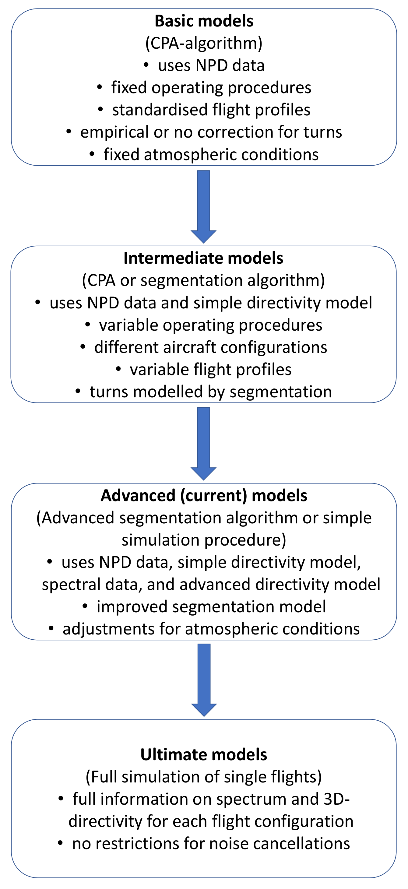
Since the 1970s, the International Civil Aviation Organization (ICAO) has introduced various standards to reduce aircraft noise at the source as part of its balanced approach to aircraft noise management. As part of the initiative, noise standards have been introduced for light, as well as large, propeller aircraft, and jet and supersonic aircraft, as well as helicopters and tiltrotors. The stages of model development can be categorized as shown in Figure 1, with advanced models being currently employed.
Aircraft noise models and standards have evolved over the years, mostly revolving around the empirical database approach, which feeds into a noise model engine. The aircraft noise database consists of acoustic and performance data based on noise–power–distance (NPD) relationships, which are fed into the noise engine consisting of some simplistic physics-based sound emission and propagation models. The noise engine also considers air traffic, radar, airport, and other operational data as inputs. All the operational data and database values are processed by the model engine to usually generate noise contours representing the Effective Perceived Noise Level (EPNL). The use of these emission and propagation models to quantify the perceived noise on the ground can follow three alternative methodologies, namely the closest point of approach (CPA), segmentation, and simulation.
Aviation noise standards have been developed to specify the acceptable noise limits as a function of Maximum Take-Off Mass (MTOM) for all categories of commercial fixed-wing transport aircraft. The recommended noise evaluation measure for the certification of these aircraft is the Sound Exposure Level (SEL) with 90% confidence limits [4]. The reference points for the SEL are take-off, overflight, and approach phases of the flight path. The measured noise levels are adjusted to the reference profile to calculate the EPNL, which is the time integral of the Perceived Noise Level (PNLT) over the noise event duration.
1.2. Unmanned Aircraft Specificities
In non-idle thrust conditions, most of the noise by conventional fixed-wing aircraft originates from the propulsion system, with a relatively smaller amount produced by the airframe and other components (such as the landing gear). The engines and gearboxes contribute a significant portion, along with the fans or propellers.
On the other hand, the majority of UA in operation belong to the category of electric Vertical Take-Off and Landing (eVTOL) aircraft. These differ very significantly from fixed-wing transport aircraft, both in terms of their nominal operating profile and in the noise emission characteristics. Whereas the bulk of the noise of conventional aircraft comes from the engine itself, the majority of eVTOL noise originates from the rotors. Traditionally, propellers and fans are characterized by axial flow (as in the case of a fixed-wing aircraft), whereas rotors most often operate in sideslip conditions (as in the case of a helicopter). Most eVTOL have multiple rotors aligned along the vertical axis, with the added provision to fly as a fixed-wing aircraft provided in some. Comparisons between a small single-engine manned aircraft and a small UA show that the UA, on average, has a larger endurance, lower fuel consumption and emissions, and has noise levels that are 6 to 9 dB lower [5]. However, with an increasing number of UA anticipated to fly at lower altitudes (<40 m AGL) in dense urban communities [6,7,8], the cumulative noise pollution for extended time periods poses grave health and wellbeing risks [3].
Considering the very different weight, flight profile, and operational environment specificities of eVTOL, simple corrections to current aviation noise models would not suffice. Consequently, the aviation research and development community has begun to develop noise emission standards for UA. The basic noise emission standard EN ISO 3744:2010 is supplemented with the installation and mounting conditions for a UA [9]. The test operating conditions are defined where the noise tests are carried out for the hovering manoeuvre of the unmanned aircraft under MTOM. The A-weighted surface time-averaged SPL is determined multiple times until the difference between at least two of the measured values does not differ by more than 1 dB.
1.3. Problem Statement
This paper addresses the gap associated with the lack of noise modelling and certification standards for UA and UAM. This objective is achieved by analysing the most relevant factors affecting the perceived noise of these platforms in typical operating conditions and using them to identify the most promising approach for the development of reliable and accurate models. These models can then be exploited to determine the ideal location of vertiports or the optimal operating settings and trajectories to be flown in order to minimize the noise perceived by the human population exposed to it.
The aircraft noise problem encompasses four fundamental aspects: the noise source itself, the flight path followed by the source, the atmospheric propagation effects, and the receiver (the human listener). As shown in Figure 2, several further considerations are relevant, and their interactions can be complex.
Therefore, in order to determine a flight path that minimises noise exposure to humans, multiple aspects must be considered. Firstly, there is the physics-based sound propagation model, which can be applied on the acoustic output from the vehicle and considers the paths it takes through the atmosphere. Secondly, this sound is heard by a listener, who effectively filters the sound relative to other noise they hear at the time, as well as by their own perception and response to the noise (psychoacoustics). This human response can supplement the propagation model to predict the equivalent sound exposure on the ground as effectively perceived by humans. Finally, these models and their numerical results can be used to calculate a more optimal flight path that would cause the smallest acoustic disturbance. All aspects of this problem must be considered for effective noise mitigation.
The focus of this article is on the sound propagation effects, with emphasis on the factors showing dependence on the flight path. Atmospheric conditions, both steady and unsteady, are only simplistically considered by conventional aircraft noise models, but can be accurately captured as part of Computational Fluid Dynamics (CFD) simulations, which however are complex and time-consuming to setup and carry out. CFD simulations also do not allow for the production of a set of results in a single run that are applicable to a range of environmental and operational conditions, so, despite their great accuracy, their exploitation for quantifying noise impacts on the ground is limited to some design trade-off studies, such as the ideal location of a new airport or runway.
Steady and unsteady propagations effects, nonetheless, have a very important impact on the SPL measured on the ground, and need to be considered for an increased accuracy of noise models in a broader set of environmental and operational conditions. Additionally, physics-based models also allow us to better account for platform dynamics and sound-reflecting surfaces, such as buildings and ground surfaces. In traditional aircraft noise propagation models, several of these factors are overlooked, or they are assumed to follow rather simplistic idealized models. The considerations introduced in the next sections of this paper allow for the consideration of some of the variables that are generally either neglected or assumed to be constant. Although some propagation effects, such as diffraction and multipath, may result in extreme complexities and thus may be omitted from surrogate models, other effects, such as wind, the temperature profile, turbulence, and Doppler effects, can be accounted for without requiring a complex CFD simulation.
The aircraft noise at the source is discussed for conventional aircraft, and the lack of sufficient data to support noise certification for UAM operations is also highlighted. The human noise perception, along with the psychoacoustic effects, is briefly discussed. The paper also discusses the flight path dependencies on the perceived noise, along with the trajectory optimization for reduced noise impacts. Some recent advances in noise certification standards for UA and their integration in the flight information management systems are discussed, before the paper concludes with a proposed future pathway for UA noise measurement and certification standards, while also discussing the reduction in aircraft noise at the source.
2. Sound Propagation
2.1. Fundamental Definitions
It is important to first consider the physics of the acoustic waves in order to address sound propagation in the atmosphere. Acoustic waves are longitudinal waves that require a material medium to propagate. Fundamentally, sound can be defined as mechanical energy transmitted by pressure waves in a material medium. In the case of sound in air, acoustic energy is transmitted from the source to the surroundings by the vibration of air particles. Sound propagates due to the transfer of energy from one vibrating particle to the next as progressive waves, with particle displacements taking place in the same direction as the movement of the wave. The velocity of sound in a medium (cm) varies with the bulk modulus (B) and density (ρ) of the medium, as shown in Equation (1). Sound travels faster in a medium with a high bulk modulus or stiffness, such as solids, as compared to a medium with a lower bulk modulus, such as fluids.
The region of travel of acoustic waves is referred to as the sound field, whereas the space where the acoustic waves propagate freely without reflection, termed free progressive waves, is called a free field. The to and fro displacement of the air particles about their mean position produces a local compression followed by a local rarefaction, and so on. The instantaneous value of the fluctuating pressure disturbance on the ambient pressure is referred to as the sound pressure and is denoted by p′. It requires a time period T to complete one cycle of compression and rarefaction, where the sound pressure at any given time t is equal to:
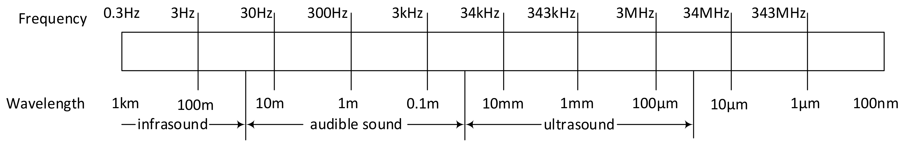
Humans can normally hear frequencies in the range of 20 Hz to 20 kHz. Consequently, frequencies lower than 20 Hz are referred to as infrasound, whereas frequencies greater than 20 kHz are called ultrasound. Figure 3 shows the frequencies and corresponding wavelengths of sound.
The sound pressure motion is a simple harmonic motion, and hence can be described in the form of a sinusoid. Sound pressure is a function of both time and distance from the source. For a point source, the variation of the sound pressure with time and distance can be expressed as:
where A is the strength of the source in dB and ω is the angular frequency in radians per second. As the sound travels with speed c, the time taken by the sound to travel a distance r is given by r/c. Since the magnitude of the sound pressure varies continuously with time, the effective sound pressure (pe) magnitude is usually given by the root mean square value of the instantaneous sound pressures over one period.
Hence, the ratio of the effective sound pressure to the local sound pressure is given by the factor √2 and is known as the crest factor of a sound signal. The attenuation rate of sound waves varies with frequency, with higher frequencies attenuating at a faster rate. Attenuation can occur either due to reflection/scattering at interfaces or absorption [10]. However, higher frequencies, having short wavelengths, reflect strongly from small objects. Reflection from surfaces causes interference with the incident sound wave, which could be constructive or destructive. Interference depends upon the frequency of sound, as well as the difference between the path length of direct and reflection paths [11]. Furthermore, the speed of sound in air varies with temperature, pressure, humidity, and wind, thereby affecting the propagation of sound. The generic equation for sound propagation can be given by [12]:
where:
- :
- The sound pressure level at distance from the source [dB];
- :
- The sound power level of the source [dB];
- :
- The combination of modifying factors that either attenuate or enhance the transmission of the sound energy as it propagates from source to receiver.
Sound can be heard around corners and behind the walls, as well due to the bending of sound waves around obstacles due to diffraction. Acoustic sources have both far-field and near-field regions. Wavefronts produced by the sound source in the near-field are not parallel and the intensity of the wave oscillates with the range and the angle between sources. The sound pressure varies with distance as a complex function of the radiation characteristics of the source. However, in the far-field, wavefronts are nearly parallel, with the intensity varying only with range to a centroid between sound sources, in accordance with the inverse squared rule. SPL, or Lp, in decibel is defined as:
where pe0 is the reference pressure of 2 × 10⁻⁵ N/m2. Analogous to Ohm’s law, in the free field, the effective pressure and the sound intensity in the direction of propagation are related, as shown in Equation (7), where ρ is the density of air:
For two independent sound sources emitting the same frequency, the resultant SPL depends on the phase difference between the two sound waves.
where . If the two sound sources are in phase, cos ωΔr/c = 1, giving:
If the two sounds are out of phase, cos ωΔr/c = −1, thus giving:
The total SPL produced by N sound sources is given by:
Similarly, SEL (LAE) and EPNL (LEPN) can be written as:
where LA,max and LPNT,max are the thresholds for SEL and EPNL, respectively, te is the effective duration, and t0 is the refence time.
2.2. Atmospheric Effects on Sound Propagation
Generally, due to thermo-fluid dynamics and molecular processes, the atmosphere acts as a low pass filter for the noise propagation spectrum. Assuming a point source of sound in an unbounded homogenous atmosphere, the propagation of sound is affected by just two attenuating effects. While the first attenuation effect is geometric, which is solely dependent on the distance from the sound source, the second effect is due to molecular absorption. In particular, sound propagates due to the oscillation of air molecules about their mean position, with a higher frequency of sound leading to a higher rate of oscillation. This vibration of the air molecules leads to loss of energy through two dissipative mechanisms. Whereas one of the mechanisms comprises frictional losses, which includes both viscous action and heat conduction, the other mechanism involves the interaction of water vapour with the resonance of oxygen and nitrogen molecules. Hence, there are heat conduction losses, shear viscosity losses, and molecular relaxation losses [13].
2.2.1. Molecular Absorption
Air absorption becomes significant at higher frequencies and at long ranges, thereby acting as a low-pass filter at a long range. The pressure of a planar sound wave at a distance x from a point of pressure P0 is given by:
The attenuation coefficient, α, for air absorption depends on the frequency, humidity, temperature, and pressure, with its value being calculated using Equation (15) [14].
where f is the frequency, T is the absolute temperature of the atmosphere in kelvins, T0 is the reference value of T (293.15 K), and fr,N and fr,O are relaxation frequencies associated with the vibration of nitrogen and oxygen molecules, respectively.
2.2.2. Temperature, Pressure and Relative Humidity Effects
The speed of sound in air varies with the temperature, relative humidity (h), carbon dioxide content (hc), and barometric pressure. A generalised empirical equation for the same is given by [15,16]:
where c and c0 are the sound speed and the reference dry-air sound speed, respectively, and a0–a12 are coefficient constants given in Table 1. The sound speed can be deducted by multiplying Equation (16) by the corresponding reference dry-air sound speed c0. For a real gas at standard pressure (101.325 kPa), the dry-air sound speed can be approximated to be 331.29 m/s, with an uncertainty of approximately 200 ppm [17], which encompasses sound speeds from 331.224 to 331.356 m/s [18].
Atmospheric effects, such as temperature variations, can affect the speed of sound and, consequently, the sound propagation in the atmosphere. In the International Standard Atmosphere (ISA), the troposphere typically extends up to 11 km. The temperature gradient in the troposphere is frequently assumed to be constant, which, however is not representative of many real conditions, and this is one important reason why conventional aviation noise models fail to account for thermal inversion layers and other anomalies affecting the temperature and relative humidity profiles. In the case of ISA and other constant tropospheric temperature gradients, the variation of the speed of sound due to the temperature [19] is given by:
where:
- c0:
- Speed of sound at sea-level;
- H:
- Height above sea-level;
- = :
- The gradient of the speed of sound, where T0 is the sea-level temperature (in Kelvin) and is the variation of temperature with height. The variation of the speed of sound due to wind (cw) is given by:
- :
- Speed of sound relative to air;
- :
- Angle of wavefront normal with the horizontal;
- :
- Horizontal wind velocity.
2.2.3. Wind and Turbulence Effects
The magnitude of the horizontal wind velocity near the Earth’s surface is predominantly determined by the prevailing horizontal pressure gradient in the atmosphere and the surface friction [19] as well as Coriolis effect. Surface friction affects the relative motion between the air and ground surface and must be accounted for heights of up to at least 1000 m.
The bending of sound also occurs due to temperature and wind gradients in the atmosphere. As a result of the uneven heating of the Earth’s surface, the atmosphere is constantly in motion. The turbulent flow of air across the rough solid surface of the Earth generates a boundary layer. This Atmospheric Boundary Layer (ABL) extends up to 5 km above ground level depending on surface heating, climatic conditions, and terrain [20]. The turbulence fluxes increase rapidly at lower altitudes closer to the ground. The flow in that region is dominated by horizontal transport of atmospheric properties. As air travels over buildings and various obstacles, there will be a local increase in wind speed due to favourable pressure gradients, in addition to significant vortex shedding. Walshe (1972) described the variation of the turbulence intensity with height and terrain, where it was shown that intensities can reach >15% at a low altitude in suburban environments [21]. Roth (2000) provided a comprehensive review of turbulence in cities [22]. It was shown that cities can attain turbulence intensities >40% within 10’s of meters Above Ground Level (AGL). Apart from the stability and control issues faced [23,24,25], the acoustic noise generated will differ because of turbulence.
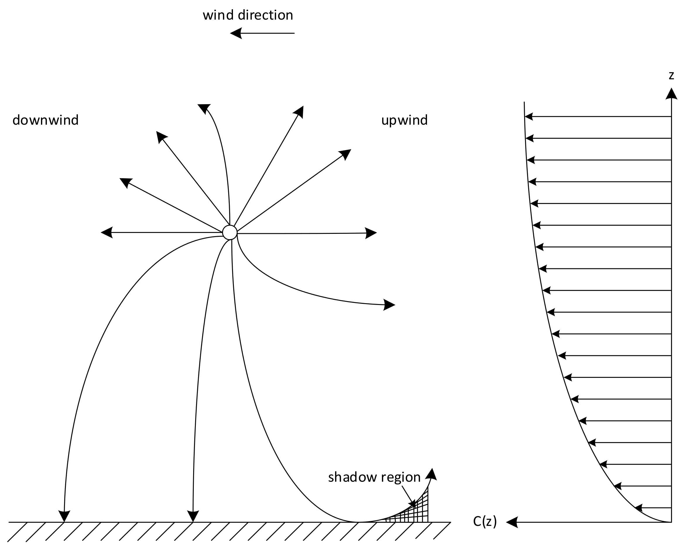
Turbulence can be modelled as a series of moving eddies with a distribution of sizes. Various turbulence models, such as Gaussian, Von Kármán, and Kolmogorov, are used in atmospheric acoustics [26,27,28]. It has been shown that turbulence effects decrease with an increase in the elevation of sound sources from the ground [29]. At lower altitudes, such models may be unsuitable for modelling the large-scale gusts induced in the wake of large infrastructure (such as buildings). Turbulence and gust imparting on the surface of the UA or ingestion by the propulsion system (such as propellers) can also influence the source noise emissions, thereby further adding to the complexity of the problem. As the temperature decreases with height, i.e., for a negative temperature gradient, in the absence of wind, sound waves bend or refract upwards due to the top of the wavefront travelling slower than the bottom. Such conditions usually exist during daytime on sunny days, leading to the formation of shadow zones. Figure 4 shows the refraction of sound due to the wind gradient. A convenient measure of turbulence in the atmosphere is by a dimensionless number known as the Richardson number. The flow is defined as turbulent for values of the Richardson number less than 1 and laminar for values greater than 1 [30].
The wind velocity either adds or subtracts from the velocity of sound, depending upon whether the source is upwind or downwind of the receiver, the height above ground, and temperature inversions. Sound is deflected towards regions of lower velocity, so, with a typical wind profile of an increasing wind speed with height, there is an upward bending of the sound with a shadow region upwind and a bending towards the ground in the downward direction. Wind effects tend to dominate over temperature effects when both are present. In the presence of both temperature and velocity gradients, the bending of sound in the direction of the wind is counteracted by a negative temperature gradient, while the shadow formation intensifies in the upwind direction. The general relationship between the speed of the sound profile c(z), the temperature profile T(z), and the wind speed profile u(z) in the direction of sound propagation, for a height z, is given by [31]:
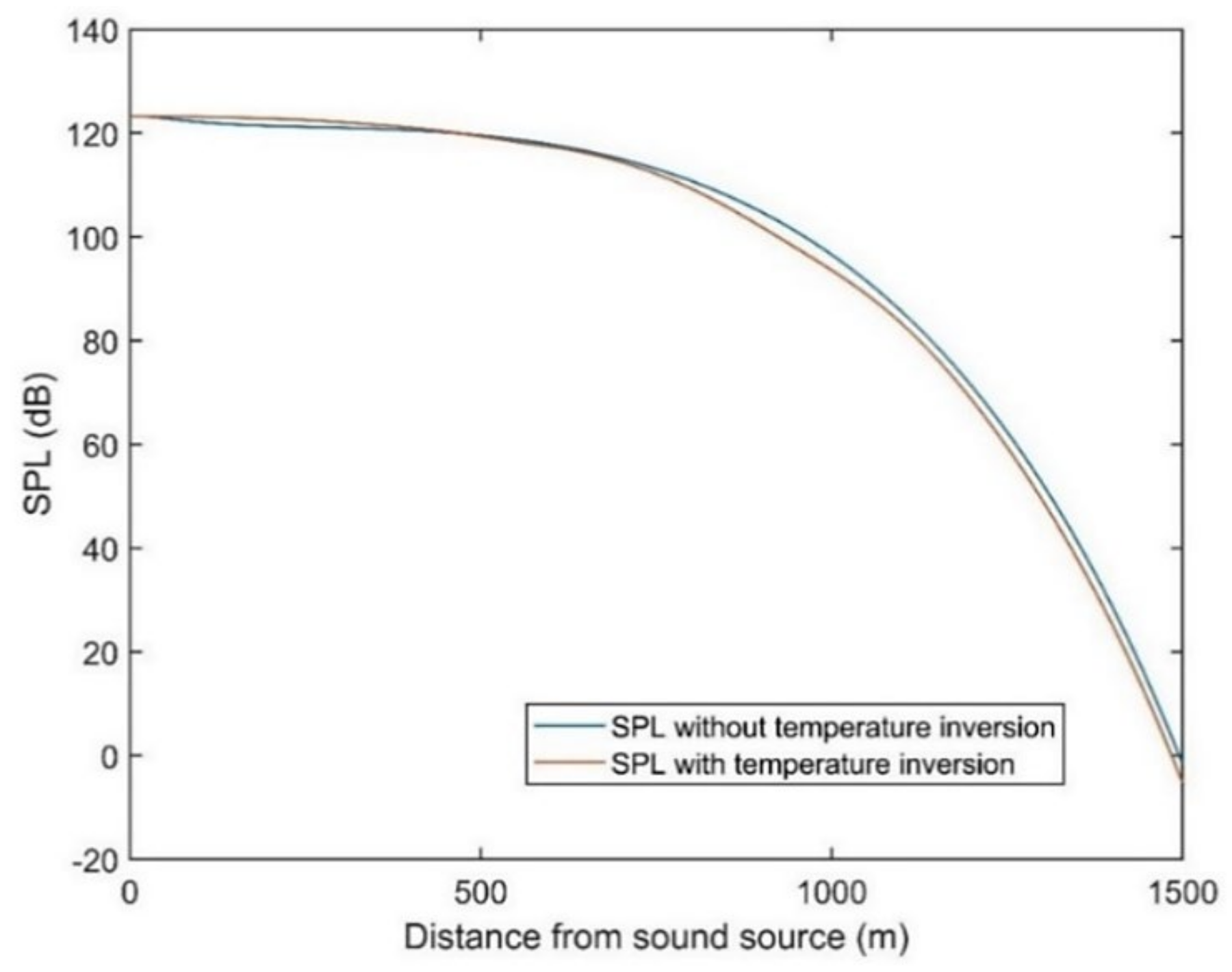
The variation of SPL with distance from the sound source, with and without temperature inversion, is shown in Figure 5. Under normal conditions, the air temperature decreases with height, following a linear relationship. However, as a layer of warm air is overlaid over cool air, there is a reversal of the normal variation of temperature. Depending on the distance from the sound source, thermal inversion can either lead to a higher or lower intensity of sound experienced. Besides the temperature, the sound intensity from sound source to a receiver can vary due to other atmospheric effects, such as varying pressure and wind conditions.
2.2.4. Doppler Effect
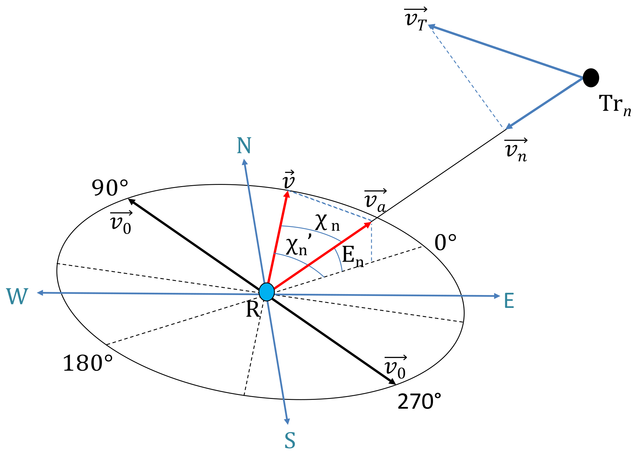
The Doppler effect is responsible for the perceived change in sound frequency due to the relative motion between the sound source and receiver. Figure 6 shows the elevation angle (En) of the nth transmitter (Trn) to the receiver (R), as well as the relative bearing (χn), the tangential velocity of the transmitter (), and the azimuth of the LOS projection (). is the velocity of the receiver and the case of results in a null Doppler shift, as no component of the receiver velocity vector is in the direction of LOS to the emitter. As is evident from Equation (22), the Doppler shift is inversely proportional to both the elevation and azimuth angle. The pitch increases as the relative distance between the sound source and receiver decreases. The change in observed frequency of sound is given as:
where:
- :
- nth receiver velocity component along the LOS;
- :
- Receiver velocity projection along the LOS;
- c:
- Speed of sound [ms−1];
- f:
- Sound frequency [Hz];
- En:
- Elevation angle of the nth transmitter;
- :
- Azimuth of the LOS projection.
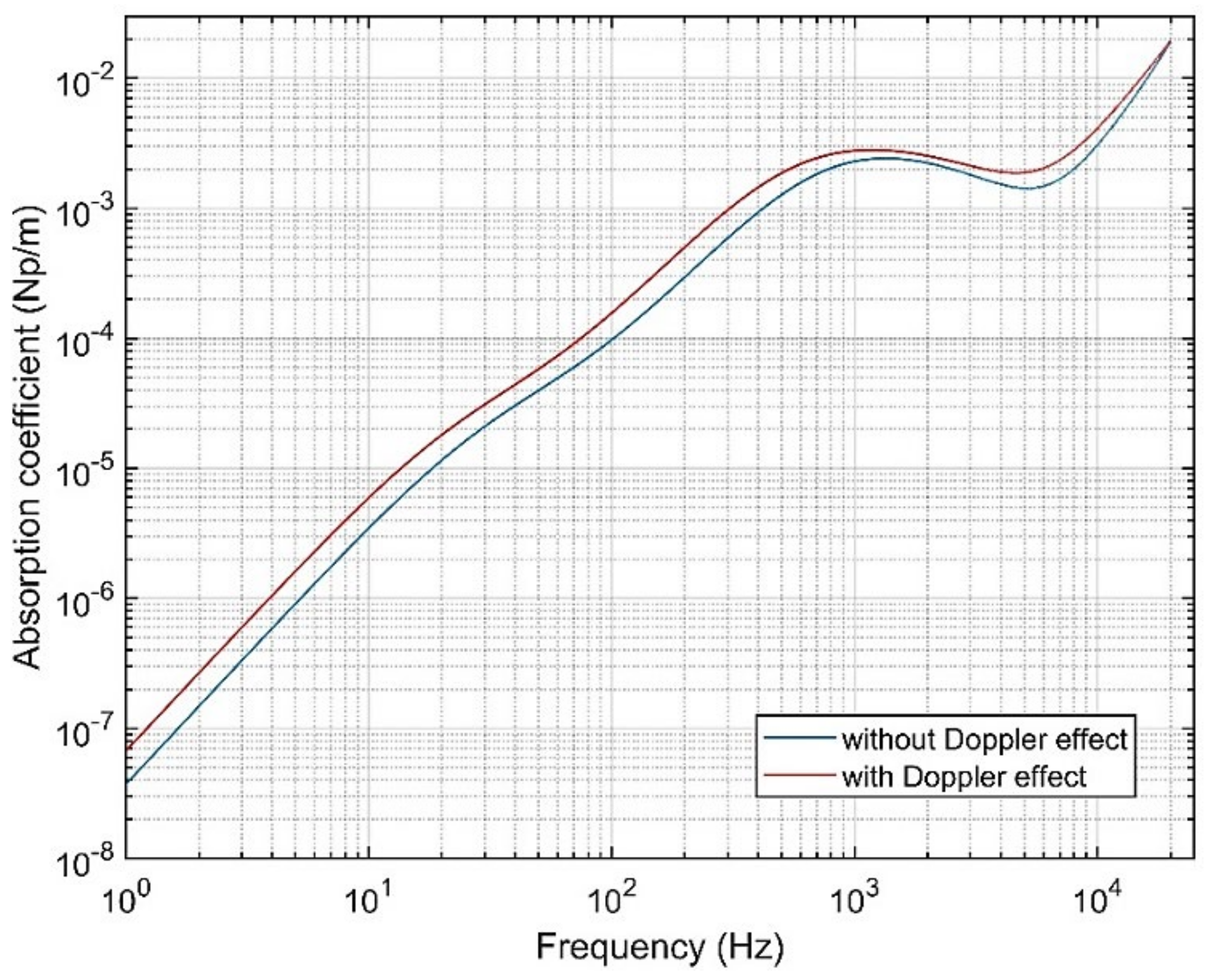
Considering a simplified case where the transmitter motion and LOS from the transmitter to the receiver are coplanar, the sound field at times t and (t + ) for a moving sound source (Tr) moves to a new point () in time . The moving sound source emits crests every units of time. The Doppler-shifted frequency from a moving sound source emitting frequency fs is given by:
where M is the Mach number for the sound source and θ is the direction of the receiver to the sound source at the time (t + ). The variation of the attenuation coefficient for air absorption, α, with frequency, while accounting for the Doppler effect, is shown in Figure 7. It can be observed that the frequency shift due to the Doppler effect for sources traveling towards the receiver increases the absorption coefficient for any given frequency.
2.3. Multipath and Diffraction around Obstacles
Urban environments are characterised by a significant number of obstacles, sometimes rising above the operating altitude of the vehicles. Researchers have therefore extended their investigation to consider multipath and diffraction phenomena affecting UA noise in urban environments. Bian et al. [33] have conducted a parametric study using a Gaussian beam tracing solver to assess the noise impact of UAs in a realistic environment. The acoustic field at observer points, which are mostly at distances greater than 10 times the rotor radius, is determined by modelling the expansion of multiple Gaussian beams. A ray-tracing module is used to determine the trajectory of each beam, with noise contributions by all beams in the vicinity of an observer point integrated to obtain the acoustic field at that point.
Ray-tracing methods, however, do not account for diffraction. Therefore, researchers [34] have modelled the actual wave physics of sound propagation through complex 3D spaces to develop immersive sound propagation models for games and mixed reality. This technique uses the cloud to translate the large number of impulse responses from the wave physics simulation into acoustic perceptually relevant parameters. It models wave effects, such as occlusion, obstruction, diffraction, and reverberation effects, and thus could potentially be applied to noise modelling in complex urban environments.
3. Sound Emission Modelling—The “Noise at Source” Problem
There are many different sources of noise in aviation, and the main source varies depending on the type of aircraft. For example, a passenger jet will make a very different noise in comparison to a helicopter or training aircraft. Noise can be generated either mechanically or aerodynamically. Mechanical noise includes sources such as bearings or structural vibrations, whereas aerodynamically generated noise stems from airflow and can include vortex shedding noise.
Aircraft noise emissions have been historically classified depending on the source as either engine noise or airframe noise. For a conventional turbofan aircraft, engine noise is the cumulative result of emissions from the fan, core, and jet, whereas airframe noise is primarily from the interactions of the air flow with the aerostructure, including the wing and tail planes, as well as devices that extend into the airflow, such as slats, flaps, or the landing gear [35].Propeller engine noise is generated primarily by air turbulence occurring over the propeller blades and rotational noise due to oscillating pressure generated by the movement of blades through the air [31]. The dominance of one noise source over another varies with the flight phase. In the departure phase, a fixed-wing aircraft is in a state of high thrust and low speed, with the flaps, slats, and the landing gear retracted shortly after take-off. Hence, engine noise is the predominant noise source during aircraft departure. However, in the approach phase, aircraft engines are in a relatively low thrust setting, with flaps and slats deployed, and the landing gear extended in preparation for landing. Thus, for a conventional aircraft, airframe noise dominates or is as loud as the engine noise during the approach phase. Noise control, both active and passive, has been widely researched for manned aircraft. For a jet aircraft, two proven passive noise control methods employ an increasing bypass ratio and fitting chevrons at the nozzle exit, whereas active noise control involves plasma actuation and fluidic injection [36].
SPL for a passenger aircraft can be computed using the Aircraft Noise and Performance (ANP) database [37]. The variation of SPL with altitude and frequency for the departure and take-off flight phases is given in Figure 8. However, the noise certification procedures developed for conventional aircraft, including rotorcraft, are not completely applicable to UA and other non-conventional aircraft. Currently, there is insufficient data to support noise certification for UAM operations [38]. Therefore, although the noise levels may be lower than those produced by conventional aircraft, UAM operations can be characterized by their novel operating mode, frequency, and other time-varying factors, which are distinctively different from conventional air traffic, and thus can be even more annoying and potentially compounded by fear and privacy concerns.
Consequently, noise reduction technologies are being developed along with noise metrics and low-noise operational procedures by regulatory bodies in collaboration with the industry and academia [39]. As most of the proposed UA will have vertical lift and forward flight capability powered by distributed electric or hybrid propulsion systems, the noise characteristics of these aircraft are expected to be different from existing helicopters and conventional general aviation aircraft. Additionally, as UA operate out of vertiports located in urban areas, their operations being in closer proximity to the noise receptors can cause serious noise concerns. These noise concerns can seriously affect the community acceptance of large-scale UA operations, which can ultimately drive the success or failure of this emerging industry.
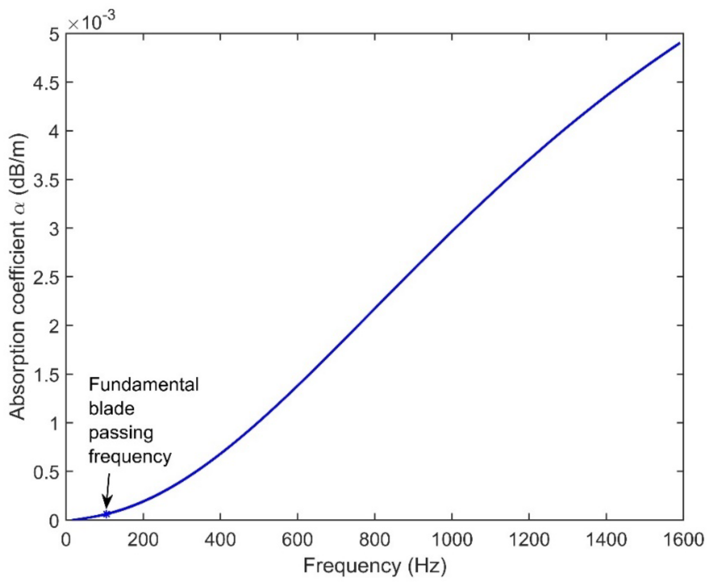
Researchers are studying the urban environment [40,41] and acoustic signature of small-scale rotors employed in the UA. The relationship between SPL and distance, the altitude, and the orientation of the UA are studied with respect to the receptor [42]. Correlation-based techniques have also been applied to quantify modulation in the acoustic field of a small-scale rotor [43]. Bi-spectral analysis has been used to reveal the correlation between the modulation strength parameters and the degree of time variation of the amplitude, with the Blade Passing Frequency (BPF) being the modulating signal and the higher-frequency noise being the carrier signal. The variation of the sound absorption coefficient (α) with a frequency for a typical small UA propeller is shown in Figure 9. It can be observed that the value of the sound absorption coefficient is quite small at the fundamental blade passing frequency and considerably increases with an increase in the propeller revolutions or number of blades.
As most of the air taxi designs are eVTOL multirotors or ultra-Short Take-off and Landing (uSTOL) vehicles, some lessons can be learnt from the noise emission from helicopters. The main source of noise for a helicopter is from its rotor blades. Blades produce several types of sound, ranging from air displacement or thickness noise, to loading noise from mostly lift and drag forces acting on the air flowing around the blade. Additionally, interactions with turbulent inflows of air and aerodynamic shocks on the blade surface also produce noise. Many air taxi designs incorporate ducted rotors, which can provide a barrier for sound.
4. Human Noise Perception
Community acceptance of UA will hinge on the impact they make in day-to-day life, and one crucial aspect of this is noise. The masking of UA noise by traffic noise from a nearby highway or railway traffic could be an effective tool for low acoustic annoyance path planning. Additionally, the perception of aircraft noise is key, and there are many factors that can influence this perception, the major one being the context during which the sound is heard. For example, the noise of an ambulance, while annoying and disruptive, is understood to be made for a very important reason (saving lives). Conversely, neighbours playing loud music very late at night is equally disruptive but is often not afforded the same allowances. The impact of perceived noise on the population is commonly described by dose–response relationships. The Awakening Index (AI) defined by the percentage of persons awakened at a specific location as a function of the perceived indoor SEL is given by:
The indoor SEL is estimated from the outdoor SEL by subtracting 20.5 dB (average loss due to the sound insulation of a typical house). The number of awakenings for a specific noise station is calculated by multiplying the percentage of awakenings of the station with the population assigned to that receiver.
A change of 5–6 dB in noise exposure can result in ”sporadic complaints” becoming ”widespread” [44]. In some cases, complaints are due to the nature or character of the sound rather than their decibel level. The frequency (pitch) of the sound is an important characteristic when considering annoyance as a response to noise, in addition to the duration of the sound. Non-acoustic effects have also shown to have a significant impact on perceived annoyance from the same sound. Moderating effects, such as the listener’s attitude towards the sound source or the activity the listener is undertaking whilst being exposed to the noise, can, in some cases, have a larger impact on annoyance than sound-exposure alone [45].
Attempts to approximate the human response to noise in objective measurements have been made with varying degrees of accuracy. One of the most common examples is the A-weighting for the decibel scale. A purely decibel scale, while common, is considered inappropriate in some circumstances because there is no weighting given to the context of the sound. A single number cannot adequately capture the character of the sound [46,47].
When it comes to specifically rating aircraft noise, energy-based descriptors have been proposed, as all sound sources in an environment can be integrated, although this approach fails to consider if the subjective meaning of each individual sound is different [48] (see the example given above about the ambulance). Helicopters are a good example of the character of the sound being distinctly different due to the phenomenon known as “blade slap”. There is evidence to suggest that this acoustic characteristic (“thumping”) is more annoying despite a lower overall SPL. However, there is an ongoing discussion on how to accurately capture this additional level of irritation in noise metrics. Several authors argue that helicopter noise should be rated no differently to fixed-wing aircraft noise [49], whereas others argue for some kind of adjustment factor [50], either overall or type-dependent [51,52].
5. Flight Path Dependencies
The take-off and landing phases are the two flight regimes during which the noise generated by an aircraft has the largest impact on ground-based listeners, both due to the closer proximity to the ground (reducing the geometric attenuation), but also because of operational specificities, such as a high thrust, deployment of high-lift devices and landing gear, and thrust reversers (increasing the noise generated at source). For this reason, a significant body of research has historically addressed the modelling, quantification, and mitigation of take-off/landing noise impacts by conventional aircraft [31,53].
The advent of UAM introduces a greater challenge, as these new vehicles and services are expected to operate much closer to densely inhabited areas (as compared to most metropolitan airports). Moreover, a much broader range of flight phases will be executed in closer proximity to the ground, with some flights occurring below the skyline and thus likely reverberating on building surfaces.
Effective noise emission and propagation models support two alternative mitigation processes:
- (1)
- The design of arrival and departure flight paths to minimize the overall noise exposure. This process requires adopting static Digital Terrain Elevation Databases (DTED) and Digital Demographic Distribution (D3) models and determining the paths that minimize the exposure levels while still being safely and practically flyable for the aircraft;
- (2)
- The definition of land use planning initiatives to limit the amount of the population potentially affected, or the extent of their exposure. This process requires assuming a predefined flight path and generating detailed “footprint”/contour maps, where, based on them, an optimal land use planning can be implemented.
Both of these processes have been commonly adopted for many decades, but one major limitation is the fact that the solutions developed are “static” in nature, thus do not consider weather and other factors that may introduce spatiotemporal anomalies in the propagation phenomena, thus potentially introducing more temporarily optimal solutions.
5.1. Trajectory Optimisation Research
Several studies have targeted noise exposure mitigation by trajectory optimization. Early studies in this subject area looked at the design/redesign of conventional arrival and departure procedures [54,55]. More recent works in this domain [56,57,58,59,60,61,62,63] opened the path for initiatives exploiting advanced navigation and guidance systems, such as Required Navigation Performance (RNP) and steep Global Navigation Satellite Systems (GNSS) arrival and approach procedures.
As mentioned in the previous paragraph, it is essential to model the aircraft’s operational capabilities in order to ensure that the optimized trajectory is ultimately flyable (and safely so). This requires implementing some aircraft performance or dynamics model, which can range from steady-state performance models to full kinematic or dynamic models [64].
Ongoing research is adopting both the simplistic empirical models as well as relatively complex and high-dimensional Computational Fluid Dynamics (CFD) simulations. In either case, the atmospheric and weather conditions are very rarely considered and, when they are treated in a typically static manner, these studies fail to capture the significant effects of the temperature, wind, air density, and other atmospheric properties on the propagation of noise generated from aircraft at various levels.
The optimizer needs to include a mathematical model of aircraft noise to allow for the minimization of perceived noise on the ground. In order to critically evaluate the noise levels, the Aviation Environmental Design Tool (AEDT) developed by the Federal Aviation Administration (FAA) serves as a multi-purpose framework integrating the Integrated Noise Model (INM) and the Model for Assessing Global Exposure to the Noise of Transport Aircraft (MAGENTA), a global noise model [65].
The concept of noise radius is adopted generally by considering the complexity of aircraft noise modelling based on the aircraft engine type, thrust setting, and atmospheric conditions [31]. The optimisation of the aircraft vertical trajectory with minimum noise impact using the analytical jet noise model has proved to be effective [63]. The methodology adopted requires demographic data at each observer location, and hence a D3 is used in conjunction with the noise model. The D3 model aids in estimating the population in a user-defined grid in a global or local scale. Additionally, the DTED is also part of the trajectory optimization framework, considering the availability of geographic information. The availability of D3 and DTED is specifically important for assessing the environmental impact of aircraft noise in the Terminal Manoeuvring Area (TMA).
Trajectory optimization is performed to avoid the densely populated areas in and around the airports, considering the topographical conditions, metrological data, and trajectory constraints. The constraints on the trajectory can be air traffic management (ATM) operational, airspace, airline, flight parameters, and/or aircraft dynamics-based constraints. Several studies have been carried out for optimizing the aircraft trajectory based on a number of cost functions, such as the number of sleep disturbances resulting in a reduction of noise annoyance on specific regions around an airport [66,67,68,69,70,71,72,73]. The reduced noise procedures implemented are Noise Abatement Departure Procedures (NADP), including NADP1, NADP2, and its associated variations, such as the ICAO-A procedure [74]. A steep trajectory approach, spiral trajectories, and touch-down displacement principles have been proposed and trialled to reduce noise while landing. Generally, the optimisation of reduced noise is not harmonious with the cost function for minimising other environmental emissions. A reduction in noise by increasing the flight time results in a higher fuel consumption and, as a consequence, higher emissions [75,76].
5.2. Monitoring and Procedure Redesign
Currently, it is generally accepted to apply the existing noise and emissions standards for manned aircraft to UA [5]. In addition, Air Navigation Service Providers (ANSPs), such as Airservices Australia, have already defined system requirements for both users and various services for a Flight Information Management System (FIMS) for UAM aircraft operations [77]. Among the system requirements for services, noise management service aims to ensure the suitable management of noise impact on the community. The noise management service hosted by FIMS shall incorporate a Noise Threshold Map (NTM), which will establish a basic grid over a geographic area and prescribe the maximum number of UA operations across different times of the day, based on various dBA level bands.
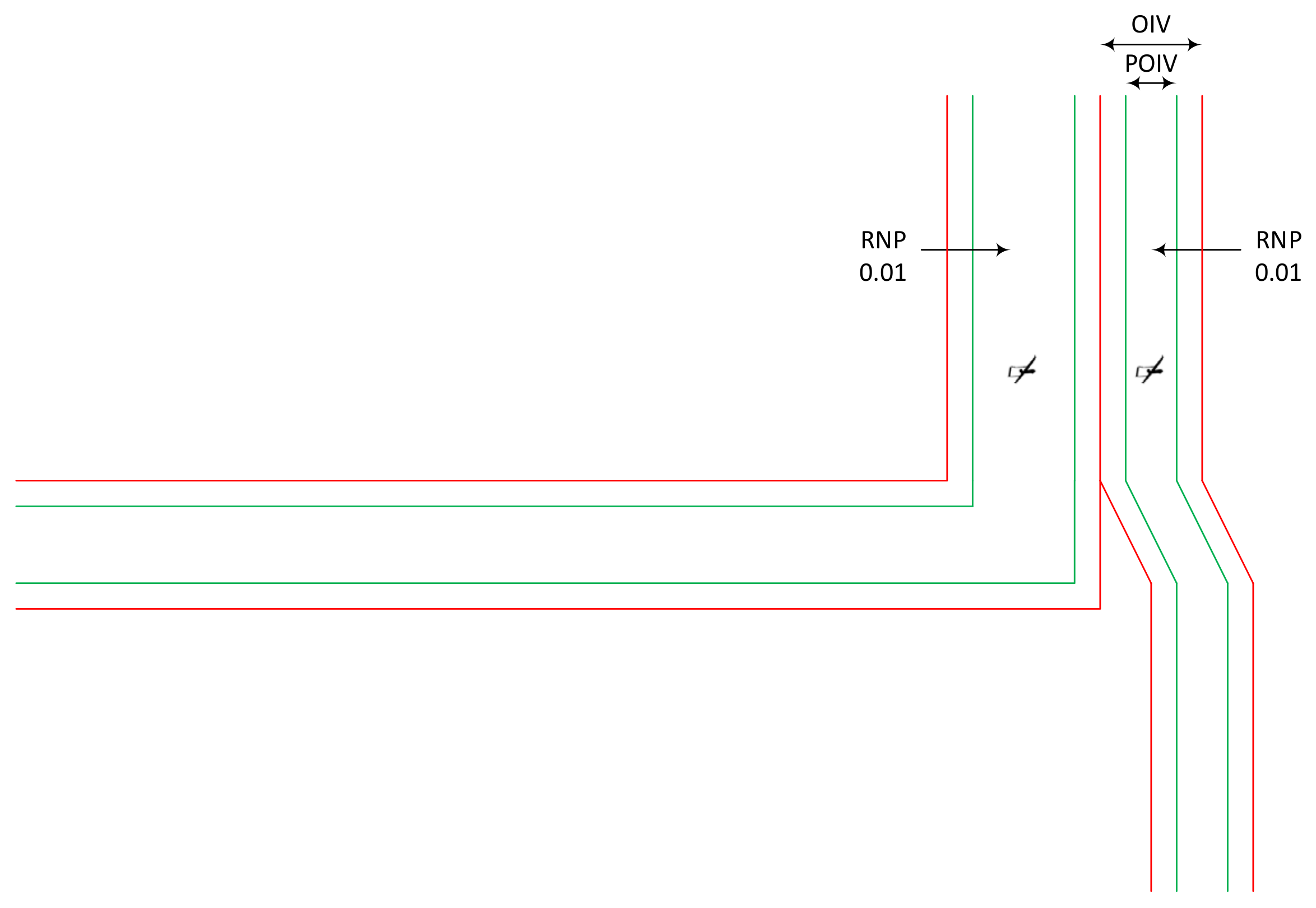
A library of acoustic parameters, such as the nominal dB output and frequency range for standard operations, shall be incorporated for different UA. All operations are consolidated into a dynamic Cumulative Noise Map (CNM), which will record both the Planned Noise Impact (PNI—before flight) and Actual Noise Impact (ANI—after flight). A free field acoustic propagation model shall be developed, which, along with the UA acoustic parameters, will be used to calculate the A-weighted sound level (dBA) at ground level along the Operational Intent Volume (OIV) centreline, which is shown schematically in Figure 10, where the Performance Operational Intent Volume (POIV) is the subset of the OIV. The ANI shall be determined through the combination of UA track data, the library of acoustic parameters, and the acoustic propagation model, and will be captured in the CNM. Besides, community inputs to the noise management service shall be allowed, along with a provision for an archival of noise data.
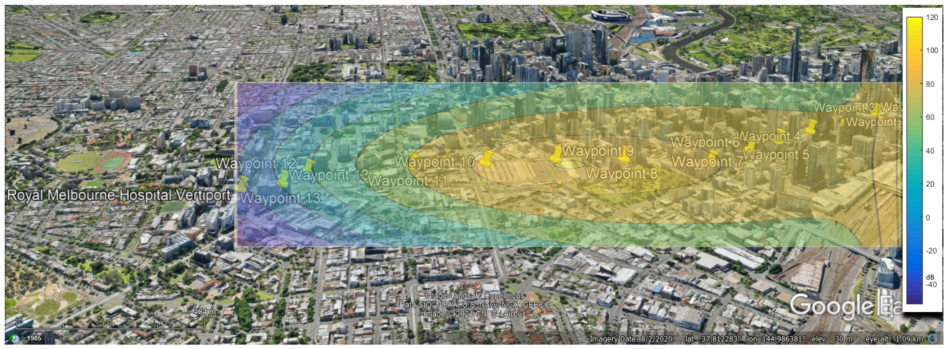
However, since the UA will be flying at low altitudes (<40 m AGL) in case of drone deliveries, and near buildings in case of “flying taxis”, there is a requirement for separate noise and emission standards for UA and small manned aircraft for urban air mobility. As the UAM framework development is currently underway, there is a strong anticipation of VTOL or uSTOL aircraft to provide UAM services in the early 2020′s [78]. However, among other constraints, UAM-generated noise, as illustratively shown in the instantaneous noise contour in Figure 11, with the yellow colour indicating a higher sound intensity that lowers as the colour changes to blue, acceptance by local communities has been identified as one of the biggest factors deterring the implementation or scaling of UAM systems.
6. Conclusions
This paper addressed the aircraft noise problem, reviewing the current noise emission, propagation, and psychoacoustic factors as they apply to manned aircraft, and the current work being carried out to develop suitable approaches for the modelling and mitigation of UA noise. Considering the unique challenges that would emerge with the widespread adoption of UAM, as well as drone delivery operations, this paper highlights the advantages of surrogate noise propagation models that both consider a broader array of environmental and operational factors as compared to legacy aircraft noise models and could potentially inform future noise certification standards for low-flying aircraft in urban environments. The physics of sound propagation reviewed in this article captures various atmospheric effects and platform dynamics, and can also support the development of simplified yet accurate multipath and diffraction models without being computationally intensive, unlike the detailed CFD models or the current noise certification standards, which either neglect atmospheric effects altogether or assume constant values.
Since noise certification is carried out for flight conditions imposed by aviation authorities, noise mitigation efforts also need to focus on the emission at the source. Fully developed surrogate sound propagation models could either inform the design of future low-flying aircraft based on their anticipated acoustic signature or aid in the path planning of an existing aircraft design for minimal noise impact. Efficient and accurate noise emission and propagation models can inform the design, development, test, and evaluation of new noise certification, as well as regulation procedures to be implemented for low-flying aircrafts in densely populated areas. Future noise certification standards for low-flying aircraft would need to consider the design improvements being undertaken to decrease the sound emission at the source. This would include improvements in the aircraft and propulsion design, as well as optimizing the flight trajectory of the UAs in order to mitigate their noise impacts on the ground, while ensuring a safe separation from other manned and unmanned aircraft. The surrogate noise models could inform the algorithms determining the flight path trajectories, as well as regulating the number of aircraft in a given airspace, based on the noise threshold set for that airspace at that particular time of the day.
Author Contributions
Conceptualisation, R.K. and R.S.; data curation, R.K.; writing-original draft preparation, R.K., N.K., A.G., A.M. and R.S; writing-review and editing, R.K., A.G. and R.S. All authors have read and agreed to the published version of the manuscript.
Funding
This research received no external funding.
Institutional Review Board Statement
Not applicable.
Informed Consent Statement
Not applicable.
Data Availability Statement
Publicly available datasets were analysed in this study. This data can be found here: https://www.aircraftnoisemodel.org/data/npd?page=112 (accessed on 24 August 2021).
Conflicts of Interest
The authors declare no conflict of interest.
References
- Casalino, D.; Diozzi, F.; Sannino, R.; Paonessa, A. Aircraft noise reduction technologies: A bibliographic review. Aerosp. Sci. Technol. 2008, 12, 1–17. [Google Scholar] [CrossRef]
- Lighthill, M.J. Jet noise. AIAA J. 1963, 1, 1507–1517. [Google Scholar] [CrossRef]
- Report on Standard Method of Computing Noise Contours around Civil Airports Volume 1: Applications Guide; European Civil Aviation Conference: Paris, France, 2016.
- International Civil Aviation Organization. Annex 16-Environmental Protection-Volume I-Aircraft Noise; International Civil Aviation Organisation: Montreal, QC, Canada, 2017. [Google Scholar]
- International Civil Aviation Organization. Unmanned Aircraft Systems (UAS); International Civil Aviation Organization: Montréal, QC, Canada, 2011. [Google Scholar]
- Watkins, S.; Burry, J.; Mohamed, A.; Marino, M.; Prudden, S.; Fisher, A.; Kloet, N.; Jakobi, T.; Clothier, R. Ten questions concerning the use of drones in urban environments. Build. Environ. 2020, 167, 106458. [Google Scholar] [CrossRef]
- Elbanhawi, M.; Mohamed, A.; Clothier, R.; Palmer, J.; Simic, M.; Watkins, S. Enabling technologies for autonomous MAV operations. Prog. Aerosp. Sci. 2017, 91, 27–52. [Google Scholar] [CrossRef]
- Mohamed, A.; Carrese, R.; Fletcher, D.; Watkins, S. Scale-resolving simulation to predict the updraught regions over buildings for MAV orographic lift soaring. J. Wind Eng. Ind. Aerodyn. 2015, 140, 34–48. [Google Scholar] [CrossRef]
- Easy Access Rules for Unmanned Aircraft Systems; European Union Aviation Safety Agency: Cologne, Germany, 2021.
- Zagzebski, J.A. Essentials of Ultrasound Physics; Mosby: Maryland Heights, MO, USA, 1996. [Google Scholar]
- Wambua, P.; Ivens, J.; Verpoest, I. Natural fibres: Can they replace glass in fibre reinforced plastics? Compos. Sci. Technol. 2003, 63, 1259–1264. [Google Scholar] [CrossRef]
- Kapoor, R.; Ramasamy, S.; Gardi, A.; Schyndel, R.V.; Sabatini, R. Acoustic Sensors for Air and Surface Navigation Applications. Sensors 2018, 18, 499. [Google Scholar] [CrossRef] [PubMed] [Green Version]
- Bass, H.; Sutherland, L.; Zuckerwar, A.; Blackstock, D.; Hester, D. Atmospheric absorption of sound: Further developments. J. Acoust. Soc. Am. 1995, 97, 680–683. [Google Scholar] [CrossRef]
- Attenborough, K. Sound propagation in the atmosphere. In Springer Handbook of Acoustics; Springer: Berlin/Heidelberg, Germany, 2014; pp. 117–155. [Google Scholar]
- Wong, G.S. Approximate equations for some acoustical and thermodynamic properties of standard air. J. Acoust. Soc. Jpn. (E) 1990, 11, 145–155. [Google Scholar] [CrossRef] [Green Version]
- Wong, G.S. Microphones and Their Calibration. In Springer Handbook of Acoustics; Springer: Berlin/Heidelberg, Germany, 2014; pp. 1061–1091. [Google Scholar]
- Wong, G.S. Speed of sound in standard air. J. Acoust. Soc. Am. 1986, 79, 1359–1366. [Google Scholar] [CrossRef]
- Wong, G.S.; Embleton, T.F.; Ehrlich, S.L. Primary pressure calibration by reciprocity. In: AIP Handbook of Condenser Microphones (Theory, Calibration, and Measurements). Acoust. Soc. Am. J. 1995, 98, 99. [Google Scholar]
- Ruijgrok, G.J. Elements of Aviation Acoustics; Delft University Press: Delft, The Netherlands, 2004. [Google Scholar]
- Garratt, J.R. The atmospheric boundary layer. Earth-Sci. Rev. 1994, 37, 89–134. [Google Scholar] [CrossRef]
- Walshe, D.E. Wind-Excited Oscillations of Structures. Wind-Tunnel Techniques for Their Investigation and Prediction; Transport and Road Research Laboratory (TRRL): London, UK, 1972. [Google Scholar]
- Roth, M. Review of atmospheric turbulence over cities. Q. J. R. Meteorol. Soc. 2000, 126, 941–990. [Google Scholar] [CrossRef]
- Mohamed, A.; Clothier, R.; Watkins, S.; Sabatini, R.; Abdulrahim, M. Fixed-wing MAV attitude stability in atmospheric turbulence, part 1: Suitability of conventional sensors. Prog. Aerosp. Sci. 2014, 70, 69–82. [Google Scholar] [CrossRef]
- Mohamed, A.; Watkins, S.; Clothier, R.; Abdulrahim, M.; Massey, K.; Sabatini, R. Fixed-wing MAV attitude stability in atmospheric turbulence—Part 2: Investigating biologically-inspired sensors. Prog. Aerosp. Sci. 2014, 71, 1–13. [Google Scholar] [CrossRef]
- Mohamed, A.; Massey, K.; Watkins, S.; Clothier, R. The attitude control of fixed-wing MAVS in turbulent environments. Prog. Aerosp. Sci. 2014, 66, 37–48. [Google Scholar] [CrossRef]
- Daigle, G.; Piercy, J.; Embleton, T. Line-of-sight propagation through atmospheric turbulence near the ground. J. Acoust. Soc. Am. 1983, 74, 1505–1513. [Google Scholar] [CrossRef]
- Juvé, D.; Blanc-Benon, P.; Chevret, P. Sound propagation through a turbulent atmosphere: Influence of the turbulence model. In Proceedings of the Sixth International Symposium on Long Range Sound Propagation, Ecully, France, 12–14 June 1994; pp. 270–282. [Google Scholar]
- Von Karman, T. Progress in the statistical theory of turbulence. Proc. Natl. Acad. Sci. USA 1948, 34, 530–539. [Google Scholar] [CrossRef] [Green Version]
- Johnson, M.A.; Raspet, R.; Bobak, M.T. A turbulence model for sound propagation from an elevated source above level ground. J. Acoust. Soc. Am. 1987, 81, 638–646. [Google Scholar] [CrossRef]
- Stull, R.B. An Introduction to Boundary Layer Meteorology; Springer Science & Business Media: Berlin/Heidelberg, Germany, 1988; Volume 13. [Google Scholar]
- Zaporozhets, O.; Tokarev, V.; Attenborough, K. Aircraft Noise: Assessment, Prediction and Control; CRC Press: Boca Raton, FL, USA, 2011. [Google Scholar]
- Sabatini, R.; Moore, T.; Ramasamy, S. Global navigation satellite systems performance analysis and augmentation strategies in aviation. Prog. Aerosp. Sci. 2017, 95, 45–98. [Google Scholar] [CrossRef]
- Bian, H.; Tan, Q.; Zhong, S.; Zhang, X. Assessment of UAM and drone noise impact on the environment based on virtual flights. Aerosp. Sci. Technol. 2021, 118, 106996. [Google Scholar] [CrossRef]
- Raghuvanshi, N.; Snyder, J. Parametric directional coding for precomputed sound propagation. ACM Trans. Graph. (TOG) 2018, 37, 1–14. [Google Scholar] [CrossRef]
- Thomas, J. Systems analysis of community noise impacts of advanced flight procedures for conventional and hybrid electric aircraft. PhD. Thesis, 2020. [Google Scholar]
- Doty, M.J.; Fuller, C.R.; Schiller, N.H.; Turner, T.L. Active Noise Control of Radiated Noise from Jets; NASA, Langley Research Center: Hampton, VA, USA, 2013.
- The Aircraft Noise and Performance (ANP) Database: An International Data Resource for Aircraft Noise Modellers. Available online: https://www.aircraftnoisemodel.org/ (accessed on 23 February 2021).
- Bent, P.; Boeing, R.; Snider, R.; Bell Flight, F. Urban Air Mobility Noise: Current Practice, Gaps, and Recommendations; NASA, Langley Research Center: Hampton, VA, USA, 2020.
- Federal Aviation Administration. Integration of Civil Unmanned Aircraft Systems (UAS) in the National Airspace System (NAS) Roadmap, 3rd ed.; Federal Aviation Administration: Washington, DC, USA, 2020.
- Prudden, S.; Fisher, A.; Marino, M.; Mohamed, A.; Watkins, S.; Wild, G. Measuring wind with small unmanned aircraft systems. J. Wind Eng. Ind. Aerodyn. 2018, 176, 197–210. [Google Scholar] [CrossRef]
- Mohamed, A.; Watkins, S.; OL, M.; Jones, A. Flight-Relevant Gusts: Computation-Derived Guidelines for Micro Air Vehicle Ground Test Unsteady Aerodynamics. J. Aircr. 2020, 58, 693–699. [Google Scholar] [CrossRef]
- Kloet, N.; Watkins, S.; Clothier, R. Acoustic signature measurement of small multi-rotor unmanned aircraft systems. Int. J. Micro Air Veh. 2017, 9, 3–14. [Google Scholar] [CrossRef]
- Baars, W.J.; Bullard, L.; Mohamed, A. Quantifying modulation in the acoustic field of a small-scale rotor using bispectral analysis. In Proceedings of the AIAA Scitech 2021 Forum, virtual event. 11 January 2021; p. 0713. [Google Scholar]
- The Social Impact of Noise; U.S. Environmental Protection Agency: Washington, DC, USA, 1971.
- Job, R. Community response to noise: A review of factors influencing the relationship between noise exposure and reaction. J. Acoust. Soc. Am. 1988, 83, 991–1001. [Google Scholar] [CrossRef]
- Michaud, D.S.; Fidell, S.; Pearsons, K.; Campbell, K.C.; Keith, S.E. Review of field studies of aircraft noise-induced sleep disturbance. J. Acoust. Soc. Am. 2007, 121, 32–41. [Google Scholar] [CrossRef] [PubMed]
- Large, S.; Stigwood, M. The noise characteristics of ‘compliant’ wind farms that adversely affect its neighbours. In Proceedings of the INTER-NOISE and NOISE-CON Congress and Conference Proceedings; Institute of Noise Control Engineering: Reston, VA, USA, 2014; Volume 249, no. 1; pp. 6269–6288. [Google Scholar]
- Namba, S. On the psychological measurement of loudness, noisiness and annoyance: A review. J. Acoust. Soc. Jpn. (E) 1987, 8, 211–222. [Google Scholar] [CrossRef]
- Molino, J.A. Should Helicopter Noise Be Measured Differently from Other Aircraft Noise? A Review of the Psychoacoustic Literature; NASA, Langley Research Center: Hampton, VA, USA, 1982.
- Leverton, J.W. Helicopter noise: Can it be adequately rated? J. Sound Vib. 1975, 43, 351–361. [Google Scholar] [CrossRef]
- Schomer, P.; Hoover, B.; Wagner, L. Human Response to Helicopter Noise: A Test of A-Weighting; US Army Corps of Engineers: Washington, DC, USA, 1991. [Google Scholar]
- Gjestland, T. Assessment of helicopter noise annoyance: A comparison between noise from helicopters and from jet aircraft. J. Sound Vib. 1994, 171, 453–458. [Google Scholar] [CrossRef]
- Ruijgrok, G.J.J. Elements of Aviation Acoustics, 2nd ed.; VSSD: Delft, The Netherlands, 2007. [Google Scholar]
- Cook, G.; Jacobson, I.; Chang, R.; Melton, R. Methodology for Multiaircraft Minimum Noise Impact Landing Trajectories. IEEE Trans. Aerosp. Electron. Syst. 1982, AES-18, 131–146. [Google Scholar] [CrossRef]
- Zaporozhets, O.I.; Tokarev, V.I. Predicted flight procedures for minimum noise impact. Appl. Acoust. 1998, 55, 129–143. [Google Scholar] [CrossRef]
- Visser, H.G.; Wijnen, R. Optimization of noise abatement arrival trajectories. Aeronaut. J. 2003, 107, 607–615. [Google Scholar]
- Visser, H.G. Generic and site-specific criteria in the optimization of noise abatement trajectories. Transp. Res. Part D Transp. Environ. 2005, 10, 405–419. [Google Scholar] [CrossRef]
- Ren, L. Modeling and Managing Separation for Noise Abatement Arrival Procedures; Massachusetts Institute of Technology: Cambridge, MA, USA, 2007. [Google Scholar]
- Hartjes, S.; Visser, H.G.; Hebly, S.J. Optimization of RNAV Noise and Emission Abatement Departure Procedures. In Proceedings of the AIAA Aviation Technology, Integration, and Operations Conference 2009 (ATIO 2009), Hilton Head, SC, USA, 21–23 September 2009. [Google Scholar]
- Prats i Menendez, X. Contributions to the Optimisation of Aircraft Noise Abatement Procedures; Universitat Politecnica de Catalunya (UPC): Barcelona, Spain, 2010. [Google Scholar]
- Prats, X.; Puig, V.; Quevedo, J.; Nejjari, F. Multi-objective optimisation for aircraft departure trajectories minimising noise annoyance. Transp. Res. Part C Emerg. Technol. 2010, 18, 975–989. [Google Scholar] [CrossRef]
- Prats, X.; Puig, V.; Quevedo, J. A multi-objective optimization strategy for designing aircraft noise abatement procedures. Case study at Girona airport. Transp. Res. Part D Transp. Environ. 2011, 16, 31–41. [Google Scholar] [CrossRef]
- Khardi, S.; Abdallah, L. Optimization approaches of aircraft flight path reducing noise: Comparison of modeling methods. Appl. Acoust. 2012, 73, 291–301. [Google Scholar] [CrossRef]
- Gardi, A.; Sabatini, R.; Ramasamy, S. Multi-objective optimisation of aircraft flight trajectories in the ATM and avionics context. Prog. Aerosp. Sci. 2016, 83, 1–36. [Google Scholar] [CrossRef]
- Noel, G.; Allaire, D.; Jacobson, S.; Willcox, K.; Cointin, R. Assessment of the Aviation Environmental Design Tool. In Proceedings of the Eighth USA/Europe Air Traffic Management Research and Development Seminar (ATM2009), Napa, CA, USA, 29 June 2009. [Google Scholar]
- Camilleri, W.; Chircop, K.; Zammit-Mangion, D.; Sabatini, R.; Sethi, V. Design and validation of a detailed aircraft performance model for trajectory optimization. In Proceedings of the AIAA Modeling and Simulation Technologies Conference, 2012 (MST 2012), Minneapolis, MN, USA, 13–16 August 2012. [Google Scholar]
- Chircop, K.; Zammit-Mangion, D.; Sabatini, R. Bi-objective pseudospectral optimal control techniques for aircraft trajectory optimisation. In Proceedings of the 28th Congress of the International Council of the Aeronautical Sciences 2012, ICAS 2012, Brisbane, Australia, 23–28 September 2012; pp. 3546–3555. [Google Scholar]
- Cooper, M.A.; Lawson, C.P.; Quaglia, D.; Zammit-Mangion, D.; Sabatini, R. Towards trajectory prediction and optimisation for energy efficiency of an aircraft with electrical and hydraulic actuation systems. In Proceedings of the 28th Congress of the International Council of the Aeronautical Sciences 2012, ICAS 2012, Brisbane, Australia, 23–28 September 2012; pp. 3757–3769. [Google Scholar]
- Gauci, J.; Zammit-Mangion, D.; Sabatini, R. Correspondence and clustering methods for image-based wing-tip collision avoidance techniques. In Proceedings of the 28th Congress of the International Council of the Aeronautical Sciences 2012, ICAS 2012, Brisbane, Australia, 23–28 September 2012; pp. 4545–4557. [Google Scholar]
- Gu, W.; Navaratne, R.; Quaglia, D.; Yu, Y.; Madani, I.; Sethi, V.; Jia, H.; Chircop, K.; Sabatini, R.; Zammit-Mangion, D. Towards the development of a multi-disciplinary flight trajectory optimization tool-GATAC. In Proceedings of the ASME Turbo Expo 2012: Turbine Technical Conference and Exposition (GT 2012), Copenhagen, Denmark, 11–15 June 2012; pp. 415–424. [Google Scholar]
- Navaratne, R.; Tessaro, M.; Gu, W.; Sethi, V.; Pilidis, P.; Sabatini, R.; Zammit-Mangion, D. Generic Framework for Multi-Disciplinary Trajectory Optimization of Aircraft and Power Plant Integrated Systems. J. Aeronaut. Aerosp. Eng. 2012, 2, 1–14. [Google Scholar] [CrossRef] [Green Version]
- Pisani, D.; Zammit-Mangion, D.; Sabatini, R. City-pair trajectory optimization in the presence of winds using the GATAC framework. In Proceedings of the AIAA Guidance, Navigation, and Control Conference 2013 (GNC 2013), Boston, MA, USA, 19–22 August 2013. [Google Scholar]
- Sammut, M.; Zammit-Mangion, D.; Sabatini, R. Optimization of fuel consumption in climb trajectories using genetic algorithm techniques. In Proceedings of the AIAA Guidance, Navigation, and Control Conference 2012 (GNC 2012), Minneapolis, MN, USA, 13–16 August 2012. [Google Scholar]
- Filippone, A. Aircraft noise prediction. Prog. Aerosp. Sci. 2014, 68, 27–63. [Google Scholar] [CrossRef]
- Prats, X.; Puig, V.; Quevedo, J. Equitable aircraft noise-abatement departure procedures. J. Guid. Control. Dyn. 2011, 34, 192–203. [Google Scholar] [CrossRef]
- Torres, R.; Chaptal, J.; Bes, C.; Hiriart-Urruty, J.-B. Optimal, environmentally friendly departure procedures for civil aircraft. J. Aircr. 2011, 48, 11–22. [Google Scholar] [CrossRef]
- Chisholm, K.C.P. FIMS (Prototype) System Requirements Specification UTM-REQ-01; Airservices Australia: Canberra, Australia, 2020. [Google Scholar]
- Vascik, P.D.; Hansman, R.J. Scaling constraints for urban air mobility operations: Air traffic control, ground infrastructure, and noise. In Proceedings of the 2018 Aviation Technology, Integration, and Operations Conference, Atlanta, GA, USA, 25–29 June 2018; p. 3849. [Google Scholar]
Figure 1.
Traditional aircraft noise modelling approach. Adapted from [3].
Figure 1.
Traditional aircraft noise modelling approach. Adapted from [3].

Figure 2.
Noise modelling flow chart.

Figure 3.
Acoustic frequencies and wavelengths.

Figure 4.
Refraction of sound due to wind gradient. Adapted from [19].
Figure 4.
Refraction of sound due to wind gradient. Adapted from [19].

Figure 5.
Variation of SPL with distance from sound source.

Figure 6.
Reference geometry for Doppler shift analysis. Adapted from [32].
Figure 6.
Reference geometry for Doppler shift analysis. Adapted from [32].

Figure 7.
Variation of absorption coefficient with frequency.

Figure 8.
Variation of SPL with altitude and frequency.

Figure 9.
Sound absorption coefficient variation with frequency.

Figure 10.
Deconflicted OIV. Adapted from [77].
Figure 10.
Deconflicted OIV. Adapted from [77].

Figure 11.
Illustrative noise contour for low-flying Urban Air Mobility aircraft.


| Coefficient Constants | Value | Unit |
|---|---|---|
| a0 | 1.000100 | – |
| a1 | 1.8286 × 10⁻³ | °C−1 |
| a2 | −1.6925 × 10⁻⁶ | °C−2 |
| a3 | −3.1066 × 10⁻³ | – |
| a4 | −7.9762 × 10⁻⁶ | °C−1 |
| a5 | 3.4000 × 10⁻⁹ | °C−2 |
| a6 | 8.9180 × 10⁻⁴ | – |
| a7 | 7.7893 × 10⁻⁵ | °C−1 |
| a8 | 1.3795 × 10⁻⁶ | °C−2 |
| a9 | 9.5330 × 10⁻⁸ | °C−3 |
| a10 | 1.2990 × 10⁻⁵ | – |
| a11 | 4.8016 × 10⁻⁵ | – |
| a12 | −1.4660 × 10⁻⁶ | °C−1 |
Publisher’s Note: MDPI stays neutral with regard to jurisdictional claims in published maps and institutional affiliations. |
© 2021 by the authors. Licensee MDPI, Basel, Switzerland. This article is an open access article distributed under the terms and conditions of the Creative Commons Attribution (CC BY) license (https://creativecommons.org/licenses/by/4.0/).
Share and Cite
MDPI and ACS Style
Kapoor, R.; Kloet, N.; Gardi, A.; Mohamed, A.; Sabatini, R. Sound Propagation Modelling for Manned and Unmanned Aircraft Noise Assessment and Mitigation: A Review. Atmosphere 2021, 12, 1424. https://doi.org/10.3390/atmos12111424
AMA Style
Kapoor R, Kloet N, Gardi A, Mohamed A, Sabatini R. Sound Propagation Modelling for Manned and Unmanned Aircraft Noise Assessment and Mitigation: A Review. Atmosphere. 2021; 12(11):1424. https://doi.org/10.3390/atmos12111424
Chicago/Turabian StyleKapoor, Rohan, Nicola Kloet, Alessandro Gardi, Abdulghani Mohamed, and Roberto Sabatini. 2021. "Sound Propagation Modelling for Manned and Unmanned Aircraft Noise Assessment and Mitigation: A Review" Atmosphere 12, no. 11: 1424. https://doi.org/10.3390/atmos12111424
Note that from the first issue of 2016, this journal uses article numbers instead of page numbers. See further details here.