2.1 CAPTEX experiment

The CAPTEX experiment consisted of seven near-surface releases of the inert tracer perfluoro-monomethyl-cyclohexane (PMCH) from Dayton, Ohio, USA, and Sudbury, Ontario, Canada, during September and October 1983 (Draxler, 1987). Table 1 lists the locations, time, amounts, and measurement counts of the seven releases. Samples were collected at 84 different measurement sites distributed from 300 to 1100 km downwind of the emission source, as either 3 or 6 h averages up to 60 h after each release (NOAA ARL, 2018a). Figure 1 shows the distribution of measurement sites and the two source locations. Release 6 is excluded from the testing as in the earlier studies using CAPTEX data (e.g., Hegarty et al., 2013; Ngan et al., 2015) due to low detection at the measurement sites. Note that 3.4 fL L⁻¹ has been subtracted from all CAPTEX measurements to remove background and “noise” in sampling where the ambient background concentration is constant at 3.0 fL L⁻¹ (Ferber et al., 1986). At ground level, 1 fL L⁻¹ is equivalent to 15.6 pg m⁻³. Duplicate sample analyses showed that the majority of the data have a mean standard deviation estimated as 10.8 % but contaminated samples may have standard deviation as large as 65 % (Ferber et al., 1986).

Table 1The locations, time, amounts, and measurement counts (M_obs) of each CAPTEX release from Dayton, Ohio, USA, and Sudbury, Ontario, Canada, during September and October 1983.

Download Print Version | Download XLSX

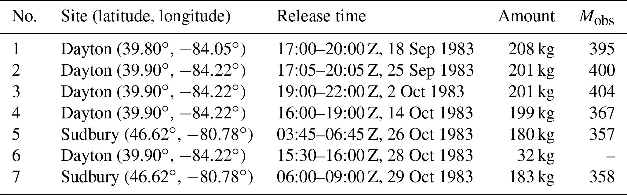
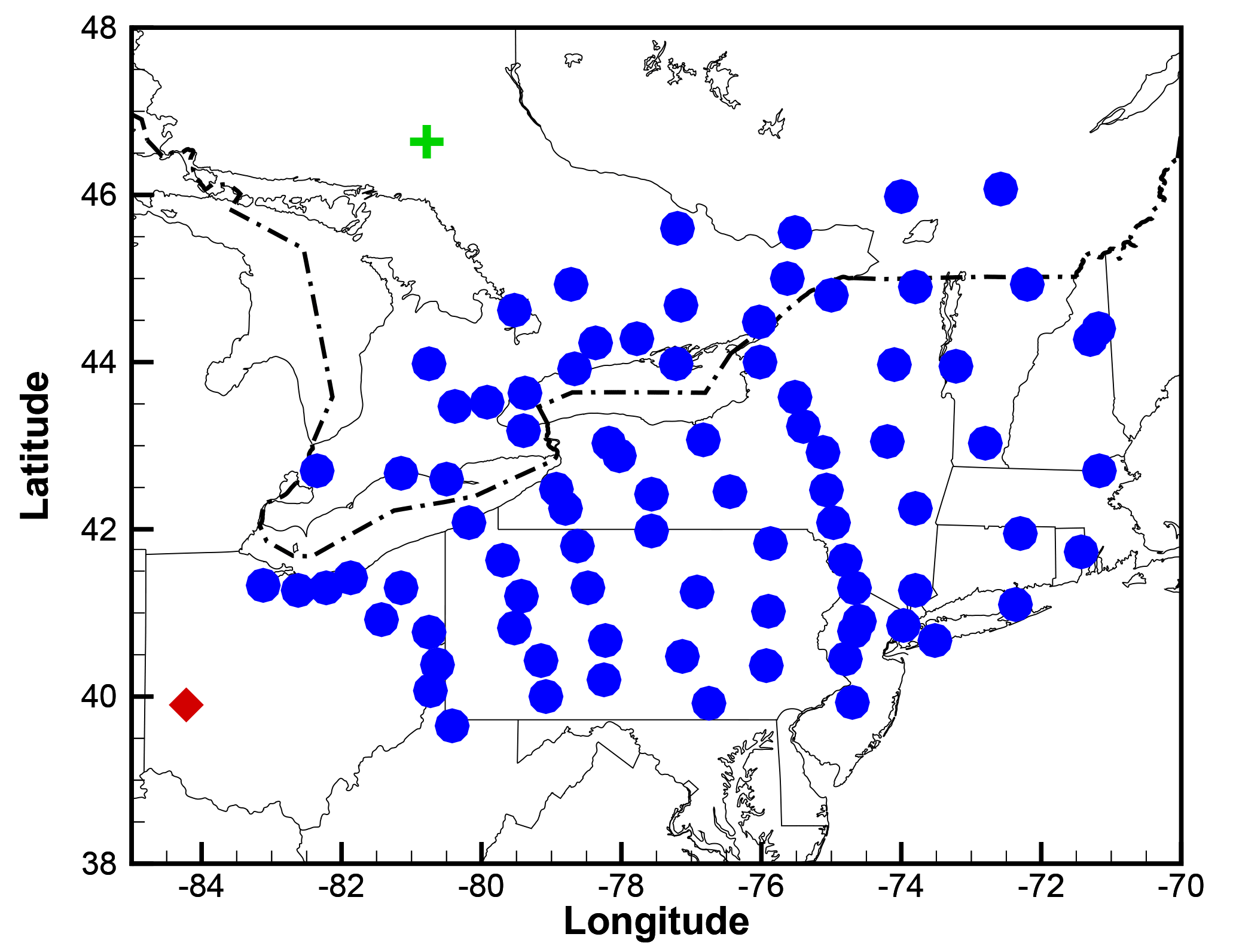
Figure 1Distribution of the 84 measurement sites and two CAPTEX source locations (Dayton, Ohio, USA, shown as a red diamond, and Sudbury, Ontario, Canada, shown as a green cross).

Download

2.2 HYSPLIT

In this study, the tracer transport and dispersion are modeled using the HYSPLIT model (version 4, NOAA ARL, 2018b) in its particle mode in which three-dimensional (3-D) Lagrangian particles released from the source location passively follow the wind field (Draxler and Hess, 1997, 1998; Stein et al., 2015). A particle release rate of 50 000 particles h⁻¹ is used for all calculations. Random velocity components based on local stability conditions are added to the mean advection velocity in the three wind component directions. The meteorological data used to drive the HYSPLIT are time averaged from the Advanced Research Weather Research and Forecasting (WRF) model (ARW, version 3.2.1) simulation results at 10 km resolution and they are identical to those used by Hegarty et al. (2013). The 10 km run was nested inside a larger domain at 30 km resolution, over which the simulation was started using the North American Regional Reanalysis (NARR) at 32 km (Mesinger et al., 2006). In the WRF simulations, 3-D grid nudging of winds was applied in the free troposphere and within the planetary boundary layer (PBL). There are 43 vertical layers, with the lowest one being approximately 33 m thick. Tracer concentrations are computed over each grid cell by summing the mass of all particles in the cell and dividing the result by the cell's volume. In this study, the concentration grid cells have 0.25^∘ resolution in both latitude and longitude directions and vertically they extend 100 m from the ground.

To avoid running the HYSPLIT modeling repeatedly, a TCM is generated similar to the previous HYSPLIT inverse modeling studies (Chai et al., 2015, 2017). As described in Draxler and Rolph (2012), independent simulations are performed with a unit emission rate from each source location and a predefined time segment. Each release scenario is simply a linear combination of the unit emission runs.

2.3 Emission inversion

Similar to Chai et al. (2015), the unknown releases can be solved by minimizing a cost functional that integrates the differences between model predictions and observations, deviations of the final solution from the first guess (a priori), as well as other relevant information written into penalty terms (Daley, 1991). For the current application, the cost functional ℱ is defined as

where q_ij is the discretized source term at hour i and location j for which an independent HYSPLIT simulation has been run and recorded in a TCM. $q_{ij}^b$ is the first guess or a priori estimate and ${\mathit{\sigma }}_{ij}^{\mathrm{2}}$ is the corresponding error variance. Note that all tracer sources in this study were at ground level and the release heights in the HYSPLIT were set as 10 m for all of the following test cases. We also assume the uncertainties of the release at each time and location are independent of each other so that only the diagonal term of the typical a priori error variance ${\mathit{\sigma }}_{ij}^{\mathrm{2}}$ appears in Eq. (1). c^h and c^o denote HYSPLIT-predicted and measured concentrations, respectively. The observational errors ${\mathit{ϵ}}_m^{\mathrm{2}}$ are assumed to be uncorrelated. As the term ${\mathit{ϵ}}_m^{\mathrm{2}}$ is essentially used to weight $(c_m^h-c_m^o{)}^{\mathrm{2}}$ terms, the uncertainties of the model predictions and the representative errors should be included in addition to the observational uncertainties. This will be further discussed in Sect. 3.2. A large-scale bound-constrained limited-memory quasi-Newton code, L-BFGS-B (Zhu et al., 1997) is used to minimize the cost functional ℱ defined in Eq. (1) when multiple parameters need to be determined. As shown by Chai et al. (2015), the metric variable can be changed from concentration to logarithm concentration. Both choices of metric variable will be tested here. Note that the cases presented in this study are all formulated as overdetermined problems.

3.1 Recovering emission strength without model uncertainty

As an initial test, the exact release location and time are both assumed known and the only unknown variable left to be determined is the release rate or the total release amount. For this type of one-dimensional problem, an optimal emission strength can be easily found without having to use sophisticated minimization routines. For instance, the ℱ may be directly calculated for a number of emission strength values, and the resulting ℱ=ℱ(q) plot will reveal the optimal q strength that is associated with the minimal ℱ. Note that such an optimal solution not only depends on the chosen parameters in Eq. 1 but also highly depends on the HYSPLIT model setup and the meteorological fields.

Both Hegarty et al. (2013) and Ngan et al. (2015) showed that the HYSPLIT dispersion model performed better for release 2 than the other releases. Thus, release 2 is initially chosen to perform a series of inverse modeling tests. Assuming no prior knowledge of the emission strength, the first guess is given as q^b=0, and σ=10⁴ kg h⁻¹ is assumed. Sensitivity tests show that when q^b is changed to 100 kg h⁻¹, the emission strength estimates are nearly unchanged with the same or larger σ.

Firstly, no model uncertainties are considered to contribute to ϵ. The observational uncertainties are formulated to include a fractional component f^o×c^o and an additive part a^o. Note that this general formulation is chosen for its simplicity. It should be replaced when more uncertainty information is available. Table 2 lists the emission strength q that generates the minimal cost function for a series of f^o and a^o combinations, where f^o ranges from 10 % to 50 %, and a^o is assigned as 10, 20, and 50 pg m⁻³. All the emission strength values obtained are significantly lower than the actual release of 67 kg h⁻¹. It shows that a larger f^o value tends to have a smaller q estimate, but a larger a^o results in a larger q. The significant underestimation of the release strength is caused by the implicit assumption of a perfect model when ϵ does not include the model uncertainties. Figure 2 shows the comparison between the predicted and measured concentrations when the actual release rate of 67 kg h⁻¹ is applied. Large discrepancies still exist even when the exact release is known and used in the simulation. For the measured zero concentrations, most of the predicted values are non-zero and can be above 1000 pg m⁻³. As ϵ_m=a^o for these zero concentrations, $\frac{(c_m^h-c_m^o{)}^{\mathrm{2}}}{{\mathit{ϵ}}_m^{\mathrm{2}}}$ will dominate the cost function when a^o is not large enough. This explains that the underestimation is not as severe for a^o=50 pg m⁻³ as that for a^o=10 pg m⁻³. While ϵ do not change with f^o for the zero concentrations, smaller f^o values help increase the weighting of the terms $\frac{(c_m^h-c_m^o{)}^{\mathrm{2}}}{{\mathit{ϵ}}_m^{\mathrm{2}}}$ associated with large measured concentrations. So, the estimated emission strength when f^o=10 % is better than when f^o=50 %.

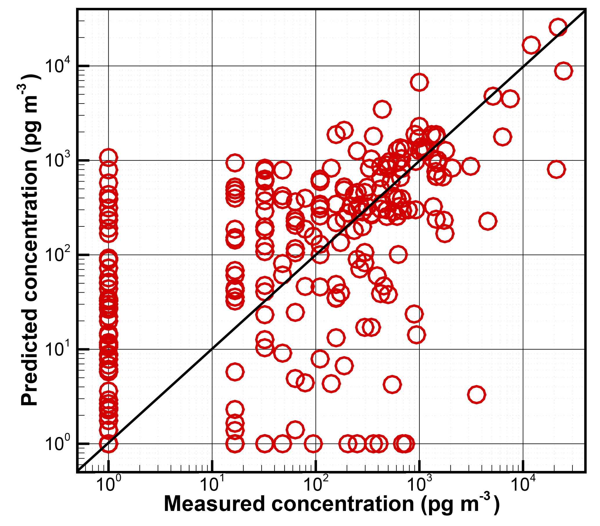
Figure 2Comparison between the predicted and measured concentrations for release 2 during the CAPTEX experiment. In the HYSPLIT simulation, at the exact release location, an emission rate of 67 kg h⁻¹ was applied from 17:00 to 20:00 Z on 25 September 1983. A constant 1 pg m⁻³ is added to both predicted and measured concentrations to allow logarithm calculation.

Download

As stated in Chai et al. (2015), the metric variable in Eq. (1) can be changed to ln(c), i.e., replacing $(c_m^h-c_m^o)$ with $\ln \left(c_m^h\right)-\ln \left(c_m^o\right)$. A constant 0.001 pg m⁻³ is added to both $c_m^h$ and $c_m^o$ to allow the logarithm operation for zero concentrations. In such a case, ${\mathit{ϵ}}_m^{\ln \left(c\right)}$ can be calculated as

Note that 0.001 pg m⁻³ is also added to $c_m^o$ in the second term to avoid dividing by zero. The $\frac{a^o}{c_m^o}$ term in Eq. (2) makes ${\mathit{ϵ}}_m^{\ln \left(c\right)}$ larger for measured low concentrations than those measured high concentrations. It causes more weighting towards measured high concentrations and results in overestimation shown in Table 3. The measured zero concentrations have little effect on the final emission strength estimates. Table 3 shows that the emission strengths are overestimated but are within a factor of 2 over the actual release of 67 kg h⁻¹, for all f^o and a^o combinations. The similar trends of how q changes with f^o and a^o are also observed here; i.e., a larger a^o or a smaller f^o tends to have a larger q estimate.

Table 2Emission strength of release 2 that minimizes ℱ for different observational errors, defined as $\mathit{ϵ}=f^o\times c^o+a^o$. Concentration is used as the metric variable.

Download Print Version | Download XLSX

Table 3Emission strength of release 2 that minimizes ℱ for different observational errors, defined as $\mathit{ϵ}=f^o\times c^o+a^o$. Logarithm concentration is chosen as the metric variable; i.e., $(c_m^h-c_m^o)$ in Eq. (1) is replaced with $\ln \left(c_m^h\right)-\ln \left(c_m^o\right)$.

Download Print Version | Download XLSX

While using logarithm concentration as the metric variable yields better emission estimates than using concentration as the metric variable, the results in Table 3 are apparently systematically overestimated compared to the systematically underestimated results in Table 2. In addition, the f^o and a^o combinations associated with the best emission estimates in Tables 2 and 3 appear to be in the opposite corners of the tables.

3.2 Recovering emission strength with model uncertainty

To consider the model uncertainties in a simplified way, ϵ² will be formulated as

As a^o and a^h affect the ϵ² in a similar way, the representative errors caused by comparing the measurements with the predicted concentrations averaged in a grid can be included in either a^h or a^o.

With logarithm concentration as the metric variable, $({\mathit{ϵ}}_m^{\ln \left(c\right)}{)}^{\mathrm{2}}$ is comprised of two parts, as

Note that a constant small number (0.001 pg m⁻³) is added to denominators $c_m^o$ and $c_m^h$ to avoid dividing by zero.

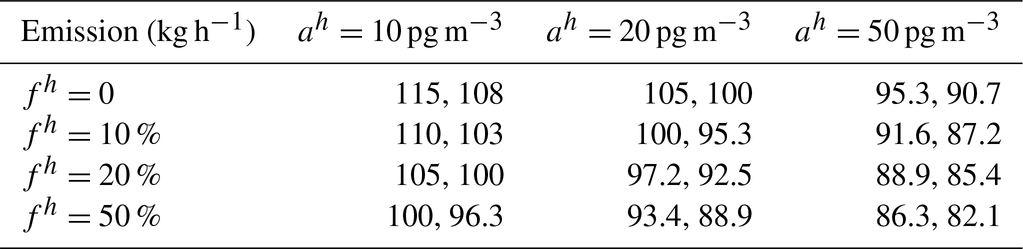
Since the predicted concentrations $c_m^h$ in Eqs. (3) and (4) will vary when source term estimates change, the model uncertainties will depend on the current release parameters. Thus, the model uncertainty terms are not static during the inverse modeling and they change along with the source estimates. Using concentration and logarithm concentration as the metric variable, respectively, Tables 4 and 5 show the emission strength estimates with different f^h and a^h, while keeping f^o=20 %, a^o=20 pg m⁻³. Additional tests with other chosen f^o and a^o values show similar but slightly different results. For brevity, they are not presented here. It should be noted that the model uncertainties are not equivalent to model errors. Although dispersion model simulations can have large errors due to various reasons including the source term uncertainties, the model uncertainties are used to indicate that the model is not perfect even with the “optimal” model parameters. Similar to the weak constraint applied in operational 4D-Var data assimilation systems (Tremolet, 2006; Zupanski, 1997), introducing model uncertainties is mainly intended to relax the model constraint for imperfect models. Here, the f^h and a^h parameters are given similar ranges to those given to the observational uncertainty parameters.

When concentration is used as the metric variable, the emission strength estimates with model uncertainties considered are improved over those without model uncertainties. The estimates of emission strength generally increase with the model uncertainty, either through a^h or f^h, except for f^h=50 %, when the q estimates slowly decreases with a^h. When f^h=0 %, a^h=10, 20, and 50 pg m⁻³, while a^o=20 pg m⁻³; the q estimates, 7.7, 9.1, and 13.6 kg h⁻¹, are in line with the results shown in Table 2, where q=7.1 kg h⁻¹ for a^o=20 pg m⁻³ and q=12.6 kg h⁻¹ for a^o=50 pg m⁻³. However, the trend of how q estimates change with f^h is opposite to how q estimates change with f^o. Table 4 shows that the emission strength increases with the model uncertainty factor f^h. With f^h=20 %, the release estimates of 48.5, 50.4, and 53.5 kg h⁻¹ are all within 30 % of the actual release rate of 67 kg h⁻¹. Instead of the underestimation shown in Table 2, the release estimates are overestimated when f^h=50 % is assumed.

With logarithm concentration as the metric variable, larger a^h or f^h results in slightly smaller q estimates. While how q estimates change with f^h is similar to how they change with f^a in Table 3, how q estimates change with a^h is opposite to how q estimates change with a^o before introducing model uncertainties. Equation (4) shows that f^o and f^h affect $({\mathit{ϵ}}_m^{\ln \left(c\right)}{)}^{\mathrm{2}}$ in a simple monotonic way, while the effect of $a_m^h$ is complicated, as it is divided by the $c_m^h$ value that varies with the source terms. Table 5 shows that the source terms are no longer overestimated as those in Table 3. In fact, all cases have slight to moderate underestimation, with the worst results being q=42.6 kg h⁻¹ when f^h=50 % and a^h=50 pg m⁻³. Another aspect of using logarithm concentration as the metric variable is that the range of the release estimates listed in Table 5 is not as large as that in Table 4, which resulted from using concentration as the metric variable for the same 12 combinations of a^h and f^h.

Table 4Emission strength of release 2 that minimizes ℱ for different f^h and a^h. Concentration is taken as the metric variable. ${\mathit{ϵ}}^{\mathrm{2}}=(f^o\times c^o+a^o{)}^{\mathrm{2}}+(f^h\times c^h+a^h{)}^{\mathrm{2}}$. f^o=20 %, a^o=20 pg m⁻³.

Download Print Version | Download XLSX

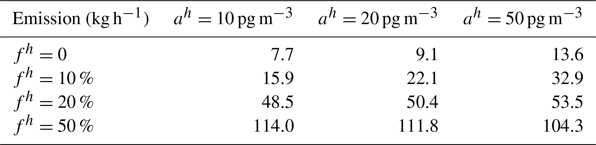
Table 5Emission strength of release 2 that minimizes ℱ for different f^h and a^h. Logarithm concentration is taken as the metric variable. $({\mathit{ϵ}}_m^{\ln \left(c\right)}{)}^{\mathrm{2}}=[\ln (\mathrm{1}+f^o+\frac{a^o}{c_m^o}){]}^{\mathrm{2}}+\left[\ln \right(\mathrm{1}+f^h+\frac{a^h}{c_m^h}){]}^{\mathrm{2}}$. f^o=20 %, a^o=20 pg m⁻³.

Download Print Version | Download XLSX

3.3 Cost function normalization

Without model uncertainties, the weighting terms for each model–observation pair do not change with emission estimates. When ${\mathit{ϵ}}_m^{\mathrm{2}}$ and $({\mathit{ϵ}}_m^{\ln \left(c\right)}{)}^{\mathrm{2}}$ are formulated as in Eqs. (3) and (4), respectively, they vary with emission estimates. This may cause complication in some circumstances when logarithm concentration is used as the metric variable. To avoid having zero source as a global minimizer in such situations, the sum of the weights of the mismatch between model simulation and observations is kept unchanged for varying q_ij by normalizing it with the weight sum when $q_{ij}=q_{ij}^b$, as shown in Eq. (5).

Figure 3 shows the cost function as a function of source strength when $({\mathit{ϵ}}_m^{\ln \left(c\right)}{)}^{\mathrm{2}}$ is defined as in Eq. (4), with f^h=0, a^h=50 pg m⁻³, f^o=10 %, a^o=20 pg m⁻³. Before introducing cost function normalization, a global minimal cost function appears when release strength approaches zero, while a local minimal cost function exists at 56.8 kg h⁻¹. Several such instances were found when a^h=50 pg m⁻³ and when f^h is 0 or 10 %, while both f^o and a^o are relatively small. The smaller cost function when release strength approaches zero is due to the increasing $({\mathit{ϵ}}_m^{\ln \left(c\right)}{)}^{\mathrm{2}}$ in Eq. (4) as $c_m^h$ gets smaller. While the model–observation differences are not smaller for lower release strength, the drastic increase of $({\mathit{ϵ}}_m^{\ln \left(c\right)}{)}^{\mathrm{2}}$ when a^h=50 pg m⁻³ and f^h is 0 % or 10 % results in smaller cost function with decreasing source strength.

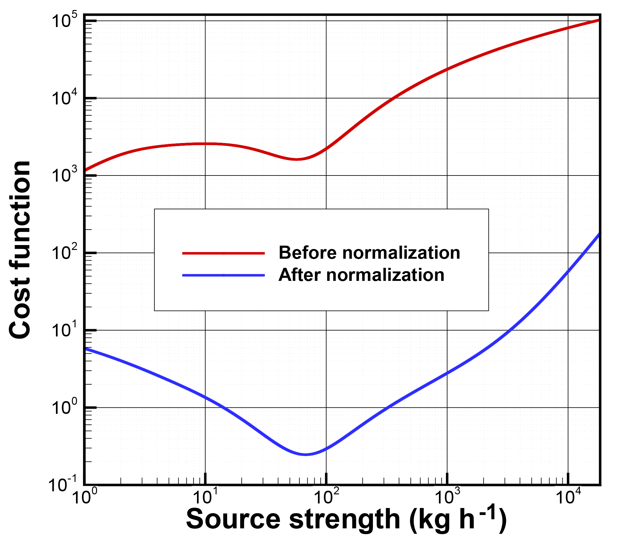
Figure 3Cost function as a function of source strength when $({\mathit{ϵ}}_m^{\ln \left(c\right)}{)}^{\mathrm{2}}$ is defined as in Eq. (4) before and after cost function normalization, with f^h=0, a^h=50 pg m⁻³, f^o=10 %, and a^o=20 pg m⁻³.

Download

Figure 3 shows that the cost function has the minimum at q=67.3 kg h⁻¹ after normalization. Note that the dramatic difference of the cost function magnitude before and after the normalization is due to the extremely small value of ${\sum }_{m=\mathrm{1}}\frac{\mathrm{1}}{{{\mathit{ϵ}}_m^b}^{\mathrm{2}}}$ calculated at q_b=0. Tables 6 and 7 show the emission strength estimates after cost function normalization with different f^h and a^h, while keeping f^o=20 %, a^o=20 pg m⁻³, using concentration and logarithm concentration as the metric variables, respectively. Note that f^o=20 % was chosen for the cases listed in Table 7, while f^o=10 % was chosen in Fig. 3 to illustrate the potential problem. How estimates change with f^h and a^h in Tables 6 and 7 is similar to what is shown in Tables 4 and 5. The estimates are generally closer to the actual release than those obtained without the cost function normalization.

When having concentration as the metric variable and with f^h=50 %, the emission strength estimates are 64.7, 64.7, and 65.3 kg h⁻¹ for a^h=10, 20, and 50 pg m⁻³, respectively. They are all within 5 % of the actual release rate. However, f^h less than or equal to 20 % results in significant underestimation. When having logarithm concentration as the metric variable, the source term estimates are not very sensitive to f^h and a^h values, and the results listed in Table 7 are all within 20 % of the actual release rate. Among those estimates, a result of 67.3 kg h⁻¹ when f^h=10 % and a^h=10 pg m⁻³ is almost identical to the actual release rate.

Table 6Emission strength of release 2 that minimizes normalized ℱ defined in Eq. (5) for different f^h and a^h. Concentration is taken as the metric variable. ${\mathit{ϵ}}^{\mathrm{2}}=(f^o\times c^o+a^o{)}^{\mathrm{2}}+(f^h\times c^h+a^h{)}^{\mathrm{2}}$. f^o=20 %, a^o=20 pg m⁻³.

Download Print Version | Download XLSX

Table 7Emission strength of release 2 that minimizes normalized ℱ defined in Eq. (5) for different f^h and a^h. Logarithm concentration is taken as the metric variable. $({\mathit{ϵ}}_m^{\ln \left(c\right)}{)}^{\mathrm{2}}=[\ln (\mathrm{1}+f^o+\frac{a^o}{c_m^o}){]}^{\mathrm{2}}+\left[\ln \right(\mathrm{1}+f^h+\frac{a^h}{c_m^h}){]}^{\mathrm{2}}$. f^o=20 %, a^o=20 pg m⁻³.

Download Print Version | Download XLSX

3.4 Ensemble

Ngan and Stein (2017) simulated CAPTEX releases using a variety of PBL schemes. In their configuration, WRF version 3.5.1 was used with 27 km grid spacing and 33 vertical layers. The NARR data set was used for the initial conditions and lateral boundary conditions. The WRF model was initialized every day at 06:00 UTC, and the first 18 h of spin-up time in the 42 h simulation were discarded. The PBL schemes used to create the WRF ensemble were the Yonsei University (Hong et al., 2006), Mellor–Yamada–Janjic (Janjic, 1994), quasi-normal scale elimination (Pergaud et al., 2009), MYNN 2.5 level TKE (Nakanishi and Niino, 2006), ACM2 (Pleim, 2007), Bougeault and Lacarrere (Bougeault and Lacarrère, 1989), University of Washington (Bretherton and Park, 2009), total energy mass flux (Angevine et al., 2010), and Grenier–Bretherton–MaCaa (Grenier and Bretherton, 2001) schemes. Nine simulations were conducted with the PBL schemes and their associated surface layer schemes, except for the YSU, BouLac, UW, and GBM cases in which the MM5 Monin–Obukhov surface scheme was applied. The land-surface model was Noah land-surface model (Chen and Dudhia, 2001), except ACM2 in which the Pleim–Xiu land-surface model was used.

An individual TCM is generated using each of the nine simulations. The nine TCMs can be used to estimate the emission strengths independently following the same procedure described previously. Tables 8 and 9 show the third (25th percentile), fifth (median), and seventh (75th percentile) emission strengths of the nine estimates that minimize the normalized ℱ defined in Eq. (5) with different f^h and a^h, while keeping f^o=20 %, a^o=20 pg m⁻³, using concentration and logarithm concentration as the metric variables, respectively. The 25th percentile and 75th percentile values are mostly within 5 % of the median estimates. While the median estimates show the same trends with f^h and a^h as the results in Tables 6 and 7, they are significantly larger due to the meteorological model differences. Apparently, the differences among the simulations with different PBL schemes are smaller than the differences between the ensemble simulations here and the simulation used in the earlier sections. This suggests that uncertainties of the emission strength are probably larger than the ranges indicated by the 25th and 75th percentile values. The results using logarithm concentration as the metric variable are quite robust with the listed model uncertainty parameters. However, the estimates using concentration as the metric variable are very sensitive to f^h and a^h. This is consistent with results shown in Sect. 3.2 and  3.3.

Instead of using each individual TCM generated from nine simulations independently, the nine TCMs can be combined into one matrix by taking the median or average values. The combined TCM can then be used to estimate the source terms. The results for concentration and logarithm concentration metric variables are listed in Tables 10 and 11, respectively. They show that the emission estimates using the median transfer coefficients of the nine TCMs are very close to the median of the nine estimates using the nine simulations individually. For the cases with logarithm concentration as the metric variable, the emission estimates using the median value of the nine TCMs are all within 3.1 % of the median values of the nine estimates obtained with each individual TCM. For the cases with concentration as the metric variable, the average relative differences are 6.4 %, with the maximum relative difference being 10.8 % when f^h=10 % and a^h=50 pg m⁻³. Combining the TCMs by taking the median value generates slightly better results than combining the TCMs by taking the average value does.

Similar to what was found in earlier sections and also in Chai et al. (2015), the cases having logarithm concentration as the metric variable generally yield better results than those having concentration as the metric variable. It is probably due to the large range of the concentrations. When having concentration as the metric variable, certain model uncertainty parameters yield good source terms, but the estimates are quite sensitive to the choices of the model uncertainty parameters. However, it is not easy to find such model uncertainty parameters that would yield satisfactory results for applications when the actual releases are indeed unknown. The results here and in the previous sections show that the estimates having logarithm concentration as the metric variable are quite robust for a reasonable range of model uncertainty parameters. For these reasons, logarithm concentration is chosen as the metric variable for the later tests.

Table 8The third (25th percentile), fifth (median), and seventh (75th percentile) emission strengths of nine simulations of release 2 that minimize the normalized ℱ defined in Eq. (5) for different f^h and a^h. Concentration is taken as the metric variable. ${\mathit{ϵ}}^{\mathrm{2}}=(f^o\times c^o+a^o{)}^{\mathrm{2}}+(f^h\times c^h+a^h{)}^{\mathrm{2}}$. f^o=20 %, a^o=20 pg m⁻³.

Download Print Version | Download XLSX

Table 9The third (25th percentile), fifth (median), and seventh (75th percentile) emission strengths of nine simulations of release 2 that minimize normalized ℱ defined in Eq. (5) for different f^h and a^h. Logarithm concentration is taken as the metric variable. $({\mathit{ϵ}}_m^{\ln \left(c\right)}{)}^{\mathrm{2}}=[\ln (\mathrm{1}+f^o+\frac{a^o}{c_m^o}){]}^{\mathrm{2}}+\left[\ln \right(\mathrm{1}+f^h+\frac{a^h}{c_m^h}){]}^{\mathrm{2}}$. f^o=20 %, a^o=20 pg m⁻³.

Download Print Version | Download XLSX

Table 10Emission strength estimates by using the average and median value of nine simulations for release 2. The cost function is normalized ℱ as in Eq. (5). Concentration is taken as the metric variable. ${\mathit{ϵ}}^{\mathrm{2}}=(f^o\times c^o+a^o{)}^{\mathrm{2}}+(f^h\times c^h+a^h{)}^{\mathrm{2}}$. f^o=20 %, a^o=20 pg m⁻³.

Download Print Version | Download XLSX

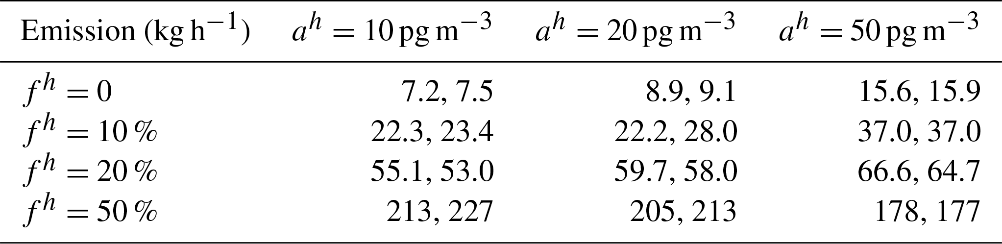
Table 11Emission strength estimates by using the average and median value of nine simulations for release 2. The cost function is normalized ℱ as in Eq. (5). Logarithm concentration is taken as the metric variable. $({\mathit{ϵ}}_m^{\ln \left(c\right)}{)}^{\mathrm{2}}=[\ln (\mathrm{1}+f^o+\frac{a^o}{c_m^o}){]}^{\mathrm{2}}+\left[\ln \right(\mathrm{1}+f^h+\frac{a^h}{c_m^h}){]}^{\mathrm{2}}$. f^o=20 %, a^o=20 pg m⁻³.

Download Print Version | Download XLSX

3.5 Source location and other releases

In addition to the source strength, the source location and its temporal variation can be retrieved with adequate accuracy using the HYSPLIT inverse system described here if there are sufficient measurements available. For instance, Chai et al. (2015) estimated 99 6 h emission rates of the radionuclide cesium-137 from the Fukushima nuclear accident using 1296 daily average air concentration measurements at 115 stations around the globe. Here, the system's capability to locate a single source location will be tested using a straightforward approach. In these tests, the release time is assumed known, but its location and strength are left to be determined. A region of suspect is first gridded at certain spatial resolution to form a limited number of candidate source locations. An optimal strength is then found at each candidate source location following the method described earlier. The location that results in the best match between the predicted and the observed concentrations is considered as the likely source location.

In the following tests, a 11×11 grid with 0.2^∘ resolution in both longitude and latitude directions is used to generate 121 candidate source locations. They are centered at 40.0^∘ N, 84.5^∘ W, for releases 1–4, and centered at 46.6^∘ N, 80.8^∘ W, for releases 5 and 7. Using the normalized ℱ defined in Eq. (5) and assuming f^o=20 %, a^o=20 pg m⁻³, f^h=20 %, and a^h=20 pg m⁻³, a minimal cost function associated with an optimal release strength can be found at each location. When logarithm concentration is taken as the metric variable, the emission estimates are not sensitive to f^h and a^h choices, as indicated by the results in Tables 7, 9, and 11. Figure 4 shows the 121 candidate locations and their respective minimal cost function values for release 2. No candidate locations are chosen to collocate with the actual source location which will be unknown for the future applications that need to locate the sources. A global minimal point is found at 39.8^∘ N, 84.5^∘ W, with ${\mathcal{F}}_{min}=\mathrm{3.14}$ achieved when q=48.5 kg h⁻¹. This grid point is taken as the estimated source location and it is 26.4 km away from the actual release site (39.90^∘ N, 84.22^∘ W). The neighboring location (39.8^∘ N, 84.3^∘ W) which is the closest to the actual release site yields a slightly larger ℱ=3.17 with an optimal release rate of 60.9 kg h⁻¹. If the exact source location is known as in the tests presented earlier, the cost function ℱ reaches 1.59 at its minimal point when q=61.5 kg h⁻¹. Apparently, compared with those cases when the release strength is the only unknown, finding both the source location and its strength with the same amount of observations is expected to be more difficult. Note that the smaller normalized ℱ values in Fig. 3 are for a case with different observation and model uncertainty parameters, where f^o=10 %, a^o=20 pg m⁻³, f^h=0 %, and a^h=50 pg m⁻³.

Table 12 lists the source location and strength estimations for the six releases following the same procedure as described here, where the uncertainty parameters are f^o=20 %, a^o=20 pg m⁻³, f^h=20 %, and a^h=20 pg m⁻³. Releases 1 and 4 have the minimal cost function ℱ_min occurring at the north boundary and the west boundary, respectively. In such scenarios, it might be necessary to expand the suspected source region for the future applications to find the source locations. However, if source locations are known to reside in the suspected region, the sources can definitely be near the boundaries. In such cases, the point with ℱ_min should be considered as the estimated source location. Releases 3, 5, and 7 have their ℱ_min occurring at inner grid points, similar to release 2 shown in Fig. 4. None of the closest candidate source locations yield the best match between model simulation and observations quantified by the cost function ℱ. Among the six releases, the estimated source location for release 2 is the closest to its actual release site, with a distance of 26.4 km.

The release rates obtained along with the likely source locations are underestimated by a factor of 3 for release 1, and overestimated by a factor of 3 for releases 4 and 7, while the estimates for releases 2, 3, and 5 are much better, with relative errors of −27.6 %, −5.4 %, and 21.5 %, respectively. Table 12 also lists the release rates q^′ estimated with the exact source location assumed known. These estimates for all releases are within a factor of 2 of the actual release rates, and the largest relative error is 53.3 % for release 1. The posterior uncertainties of the release rate estimates ${\mathit{ϵ}}_{q^{\prime }}$ are also calculated and listed. They range from 1.8 kg h⁻¹ for release 2 to 6.2 kg h⁻¹ for release 1. The apparent underestimation is likely due to the model uncertainty assumption, including its simplified formulation as well as the chosen parameter values. Either with the source location known or unknown, release 2 has one of the best emission estimates among the six releases, probably because the HYSPLIT forward model has the best performance for the same release (Hegarty et al., 2013). The significant model errors when simulating the transport and dispersion even with the exact source terms are mostly caused by the meteorological uncertainties, while the HYSPLIT physical schemes and parameters, as well as the numerical discretization, also contribute.

An assumption made in this inverse modeling algorithm is that the differences between model and observation have a normal distribution with a zero mean. Figure 5 shows the probability density function (pdf) of ln(c^h)−ln(c^o) for the six CAPTEX releases using the estimated release rate q^′ listed in Table 12. The pdf distribution of ln(c^h)−ln(c^o) for release 2 is consistent with the normal distribution assumption, and the pdf for release 4 shows the largest deviation from a normal distribution, while those for the other four releases resemble a normal distribution to some extent. The largest relative error for release 1 is likely related to the negative mean of the ln(c^h)−ln(c^o) distribution shown in Fig. 5. The overestimated q^′ probably results from the compensation of the model bias. Note that the better performance using ln(c^h)−ln(c^o) than c^h−c^o is believed to be caused by the fact that normal distribution assumption is mostly valid for the former but probably invalid for the latter.

The meteorological field and the observations are the two major inputs to the current inverse modeling. As discussed above, better model performance of release 2 helps to lead to better inverse results than the other releases. However, it is impossible to eliminate the model uncertainties. In practice, ensemble runs can be used to quantify the uncertainties and reduce the model errors by taking the average or median values of the ensemble runs. On the other hand, increasing the number of observations is effective to improve the inverse modeling results and reduce the result uncertainty. In principle, when the release strength is the only value to be determined, each measurement within the predicted plume can provide an independent estimate. However, relying on a single observation to estimate the strength is problematic since a particular model output can be very different from the observation and thus lead to an erroneous estimation of the source strength when used in isolation. For instance, although the HYSPLIT predictions of release 2 with exact source terms are very good, compared with individual measurements, they have severe underestimation (e.g., 0.77 pg m⁻³ predicted versus 686 pg m⁻³ measured), as well as significant overestimation (e.g., 2033 pg m⁻³ predicted versus 31.2 pg m⁻³ measured). Therefore, similar to a regression technique, increasing the sampling number can improve the final results, as exemplified by the very good source term estimation for release 2 when using all the available measurements. Also note that the samples outside predicted plumes do not contribute to the inverse modeling. Table 1 lists the total measurement counts for each release, but the number of measurements actually contributing to the inverse modeling are those inside the HYSPLIT plumes, including those with zero or background concentrations. The number of such effective measurements inside the plumes generated by HYSPLIT from the exact source location and time period are reduced to 148, 237, 211, 68, 46, and 53, for releases 1–5 and 7, respectively. The largest number of effective measurements, 237, of release 2, also indicates the best performance of the HYSPLIT simulation among those of the six releases. The effectiveness of the measurements will change when source location or release time is changed. The measurements that are not active in determining the source strength with a known source location and release time may be effective to locate the source locations.

Table 12The source location (latitude, longitude) and release rate q_min identified by the minimal normalized cost function ℱ_min for each CAPTEX release. A total of 121 candidate locations are prescribed with 0.2^∘ resolution in both longitude and latitude directions, centered at (40.0^∘ N, 84.5^∘ W) for releases 1–4, and at (46.6^∘ N, 80.8^∘ W) for releases 5 and 7. Δ is the distance between the point with ℱ_min and the actual release site. q^′ is the estimated release rate by assuming that the actual release location is known. ${\mathit{ϵ}}_{q^{\prime }}$ is calculated using $\frac{\mathrm{1}}{({\mathit{ϵ}}_{q^{\prime }}{)}^{\mathrm{2}}}=\frac{\mathrm{1}}{({\mathit{ϵ}}_{q^b}{)}^{\mathrm{2}}}+{\sum }_{m=\mathrm{1}}^M\frac{\mathrm{1}}{(q^{\prime }{)}^{\mathrm{2}}\times ({\mathit{ϵ}}_m^{\ln \left(c\right)}{)}^{\mathrm{2}}}$, where ${\mathit{ϵ}}_m^{\ln \left(c\right)}$ is obtained using Eq. (4). For all of the cases, f^o=20 %, a^o=20 pg m⁻³, f^h=20 %, and a^h=20 pg m⁻³. Logarithm concentration is taken as the metric variable.

Download Print Version | Download XLSX

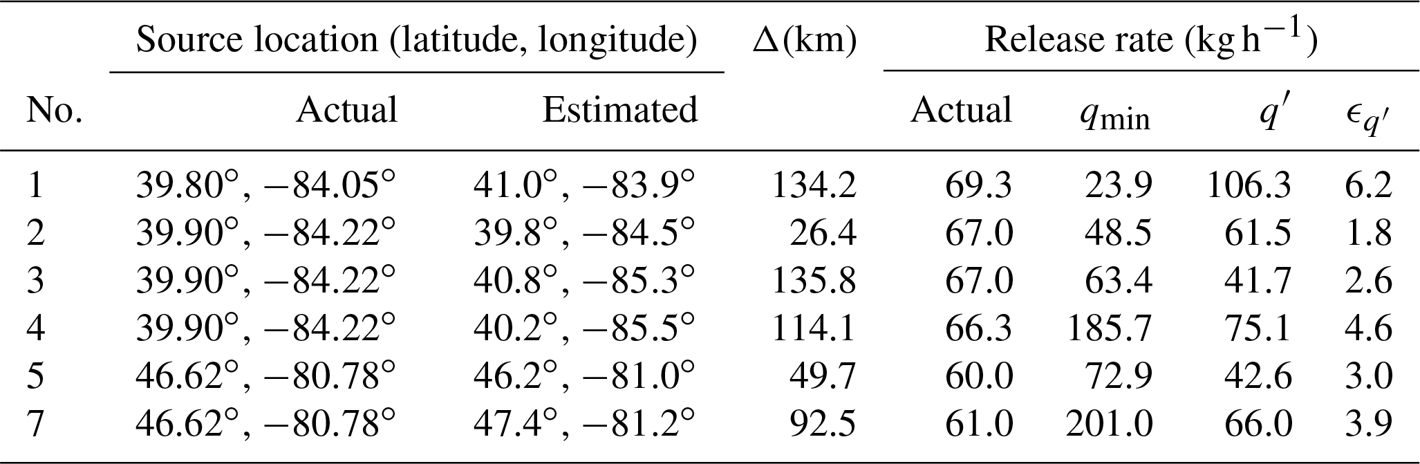
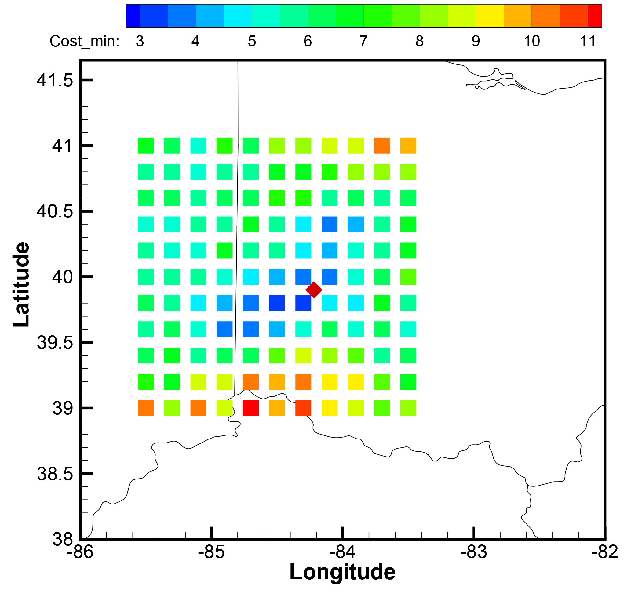
Figure 4Distribution of 121 candidate source locations for release 2. The minimal cost function at each location associated with an optimal release strength is indicated by color. The cost function defined in Eq. (5) is calculated with f^o=20 %, a^o=20 pg m⁻³, f^h=20 %, and a^h=20 pg m⁻³. The actual source location, Dayton, Ohio, USA, is shown as a red diamond.

Download

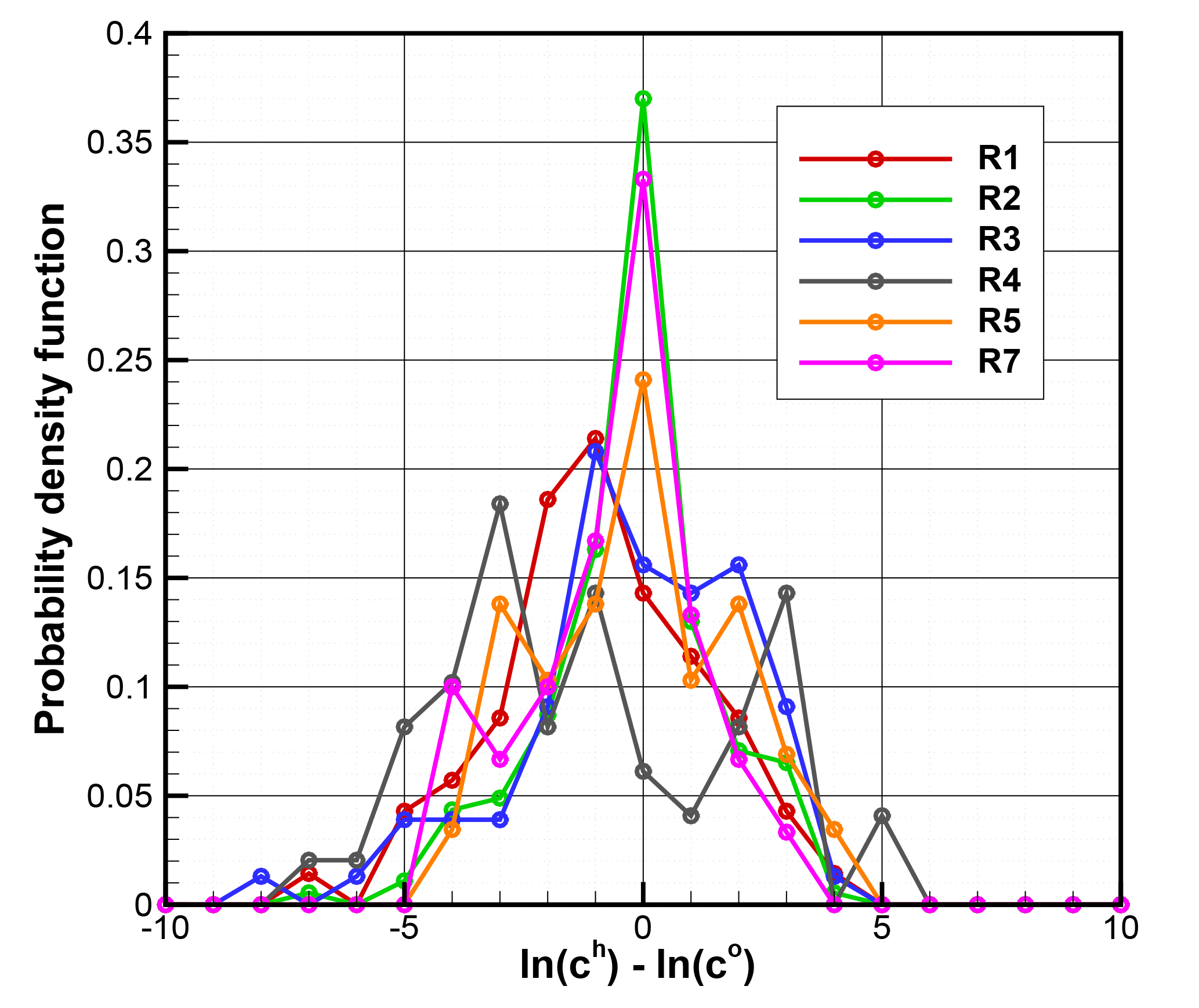
Figure 5Probability density function (pdf) of ln(c^h)−ln(c^o) for the six CAPTEX releases. Units of c^h and c^o are pg m⁻³. The model prediction c^h is calculated using the estimated release rate q^′ listed in Table 12. ln(c^h)−ln(c^o) is calculated when both c^h and c^o are non-zero. The number of data points used for pdf calculation is 70, 184, 77, 49, 29, and 30, for releases 1–5, and 7, respectively.

Download