the Creative Commons Attribution 4.0 License.
the Creative Commons Attribution 4.0 License.
 | 13 Feb 2020
glmGUI v1.0: an R-based graphical user interface and toolbox for GLM (General Lake Model) simulations
Marko Wenk
Benjamin Poschlod
Filippo Giadrossich
Mario Pirastru
Mark Vetter
Numerical modeling provides an opportunity to quantify the reaction of lakes to alterations in their environment, such as changes in climate or hydrological conditions. The one-dimensional hydrodynamic General Lake Model (GLM) is an open-source software and widely used within the limnological research community. Nevertheless, no interface to process the input data and run the model and no tools for an automatic parameter calibration yet exist. Hence, we developed glmGUI, a graphical user interface (GUI) including a toolbox for an autocalibration, parameter sensitivity analysis, and several plot options. The tool is provided as a package for the freely available scientific code language R. The model parameters can be analyzed and calibrated for the simulation output variables water temperature and lake level.
The glmGUI package is tested for two sites (lake Ammersee, Germany, and lake Baratz, Italy), distinguishing size, mixing regime, hydrology of the catchment area (i.e., the number of inflows and their runoff seasonality), and climatic conditions. A robust simulation of water temperature for both lakes (Ammersee: RMSE =1.17 ∘C; Baratz: RMSE =1.30 ∘C) is achieved by a quick automatic calibration. The quality of a water temperature simulation can be assessed immediately by means of a difference plot provided by glmGUI, which displays the distribution of the spatial (vertical) and temporal deviations. The calibration of the lake-level simulations of lake Ammersee for multiple hydrological inputs including also unknown inflows yielded a satisfactory model fit (RMSE =0.20 m). This shows that GLM can also be used to estimate the water balance of lakes correctly. The tools provided by glmGUI enable a less time-consuming and simplified parameter optimization within the calibration process. Due to this, i.e., the free availability and the implementation in a GUI, the presented R package expands the application of GLM to a broader field of lake modeling research and even beyond limnological experts.
- Article
(3289 KB) -
Supplement
(1000 KB) - BibTeX
- EndNote


Because lakes respond to changes in their environment they are often considered to be “sentinels of change” (Williamson et al., 2009; Hipsey et al., 2019). The investigation of alterations in the physical conditions of lakes, such as water temperature, stratification, water balance, mixing behavior, or ice cover, has a key role in the understanding of the lake dynamics. Numerical modeling provides an opportunity for research beyond the analysis of observational monitoring data (Frassl et al., 2016), enabling simulations of periods without in situ data as well as future conditions of lakes.
The development and application of community-based models is of increasing importance in order to find solutions for the future challenges to simulate water body conditions under environmental alterations (e.g., climatic, land use, and agricultural policies; Bruce et al., 2018). The one-dimensional hydrodynamic General Lake Model (GLM) has been developed, under the leadership of members of the Global Lake Ecological Observatory Network (GLEON, https://gleon.org, last access: 30 January 2020; Hanson et al., 2016), in response to the need of a robust model of lake dynamics (Hipsey et al., 2019), which is applicable for the vast diversity of lakes and reservoirs around the globe. GLM is able to simulate the thermal dynamics of lakes in their temporal and spatial (vertical) characteristics. The model code is open source and applied in numerous studies to a broad variety of different lakes and research questions (e.g., Bueche et al., 2017; Bucak et al., 2018; Bruce et al., 2018; Fenocchi et al., 2017, 2018, 2019; Robertson et al., 2018; Ladwig et al., 2018; Mi et al., 2018). Carey and Gougis (2017) present the usage of GLM beyond the research application by incorporating it into a teaching tool for students.
A powerful toolbox for automatic calibration, validation, and statistical sensitivity analysis is not yet existent, although GLM is often used in the research community. Therefore, we developed an R-based graphical user interface (GUI) implemented in the new R package glmGUI, combining an easy handling of GLM simulations, a tool to automate the calibration process, and visualization options for the input and output data. In general, the maxim of our project was inspired by four aspects:
-
provision of an open-source tool;
-
provision of a user-friendly tool, which could be used by experts as well as less experienced modelers and limnologists;
-
using scripts to adapt the tool, with high acceptance and contribution in the scientific community; and
-
flexibility for the implementation of different calibration parameters and for the numerical and graphical interpretation of the output results.
The R language (https://www.r-project.org, last access: 30 January 2020) was chosen because it is open source, flexible, and an independent platform (Snortheim et al., 2017). Moreover, the lake modeler community already uses R-based packages, i.e., glmtools for parameterization or plotting model output (https://github.com/USGS-R/glmtools, last access: 30 January 2020) and rLakeAnalyzer for postprocessing and evaluation of the model results (Winslow et al., 2016, https://github.com/GLEON/rLakeAnalyzer, last access: 30 January 2020).
Changes in the water level of a lake can have strong influences on hydrodynamics, such as thermocline depth and stratification stability and duration, and they can also affect lake water quality (Robertson et al., 2018). The appropriate water level reproduction by lake models is essential for a robust simulation of spatial features of thermal dynamics in lakes, especially in shallow lakes with high variations in water stages. Furthermore, an accurate simulation of the lake level ensures the correct representation of hydrological interaction of the lake with its environment in the catchment area. Hence, in addition to the model output water temperature, the lake level is included to be calibrated in the provided automated calibration tool.
In this contribution we present the options included in glmGUI, and we show the application for two different sites, namely the pre-alpine deep lake Ammersee, southern Germany, and the shallow, Mediterranean lake Baratz, Sardinia, Italy. The objectives of these two case studies are the calibration of the water temperature and lake-level simulations of GLM using the automatic calibration tool.
2.1 The hydrodynamic lake model
GLM is a one-dimensional hydrodynamic model simulating the vertical profiles of temperature, salinity, and density at one spatial point in a lake over time (Frassl et al., 2016; Robertson et al., 2018). It applies the Lagrangian layer structure adapting the thickness and volume of layers with uniform properties from each simulation step (Bueche et al., 2017). The underlying equations and hydrodynamics closures are documented in Hipsey et al. (2014, 2017). The hydrodynamic model can also easily be coupled with the Aquatic Ecodynamics library (AED2) to simulate water quality simulations (Weber et al., 2017; Bruce et al., 2018).
GLM simulations are based on parameterizations of mixing processes, surface dynamics, and the effect of inflows and outflows. The model performance for simulating the lake thermal dynamics as well as the water balance can be improved by a calibration of lake-specific parameters. The model documentation of Hipsey et al. (2017) includes also a description of the lake-specific parameters and the default values for GLM simulations. The model requires meteorological and hydrological input data (see Table A1 in Appendix A). Field data of water temperature should be available in a suitable temporal and spatial (several depths) resolution to enable a reliable calibration process.
2.2 R package glmGUI
The R package glmGUI written by the authors interacts with the functionality of GLM. It provides two basic application functions – the logical elements of model-fit criteria calculations and graphical user interfaces for data visualization. The package requires a software version of R of ≥3.4 and the version of rLakeAnalyzer ≥1.8.3. All required R packages are automatically installed during the first installation of glmGUI.
2.3 Graphical user interface
The graphical user interface is constructed as a window-based design using functions of the R package gWidgets (Verzani, 2014), which provides several toolkits for producing user interfaces by creating, for example, labels, buttons, containers, or drop lists. The GUI is organized in a main menu with five sections. Submenus and result messages are opened in separate windows (Fig. 1).
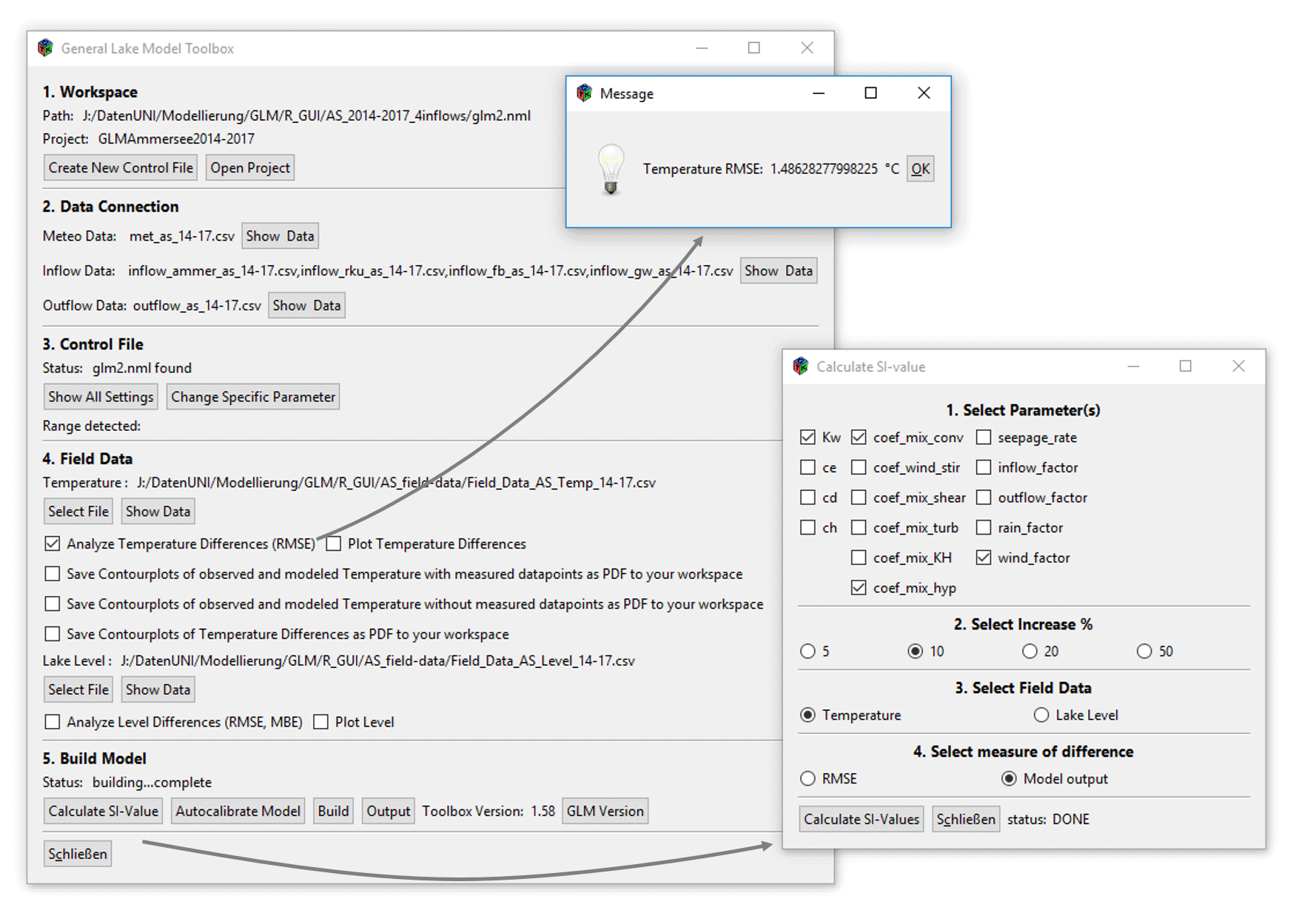
Figure 1Window-based structure of glmGUI with examples of the submenu “Calculate SI-value” and of the result message “Temperature RMSE” created after a model run.
2.3.1 Data preprocessing and model efficiency
The GUI enables either the usage of an existing simulation control file of GLM (glm2.nml) from a selectable workspace (Sect. 1, Fig. 1) or the creation of a new control file using the function nml_template_path of the R package GLMr (https://github.com/GLEON/GLMr, last access: 30 January 2020). The lake-specific parameters and settings are in accordance with the deposited file of GLMr and is due to change with the current GLM version. The input data are automatically listed in part 2 (Fig. 1) if stored at the path as specified in the control file. All included time series of input data can be visualized and tested against missing values (NA). The toolbox includes an option to fill the missing values by applying the nonparametric Kalman filter method (Grewal, 2011) using the R package imputeTS (Hyndman and Khandakar, 2007). Several filter methods were tested by manually removing values from existing time series of meteorological data and interpolating these missing values. The Kalman smoothing could deliver the best and most constant results for all kinds of various meteorological data. If selected, an autofill option writes the interpolated values directly to the input file. All parameter settings defined within the control file can be shown and changed by the GUI (part 3, Fig. 1).
The model simulation can be run (part 5, Fig. 1) and several plot options can be selected to compare the model result with observed field data (part 4, Fig. 1). As lake level variations can have a strong impact on the water temperature distribution within lakes (especially true for shallow waters), the validation of the lake-level simulation results is provided within the GUI additionally to the water temperature. The root mean square error (RMSE), which is often applied as model fit criteria in lake modeling studies (e.g., Bueche et al., 2017; Luo et al., 2018; Frassl et al., 2018), can be computed for both model output variables. Additionally, the mean bias error (MBE, average of the lake-level differences of all simulated time steps) is calculated for lake-level simulations. Both model criteria are calculated for all available observed data points and averaged subsequently.
2.3.2 Plots and output visualization
Plot options are provided by glmGUI for the input time series in part 2 (Fig. 1) and for all output variables generated by GLM (csv and netCDF file formats, part 5 Fig. 1). This includes simple line plots (e.g., for lake level or evaporation) and contour plots for a parameter varying with lake depth, such as water temperature or density. In addition, two types of contour plots of the vertical profile can be created. First is the visualization of observed and modeled water temperatures in one plot above each other with the option of the measured data as point overlay to mark where and when field data are available (areas in between are interpolated to draw the plots, Fig. 2). The second plot visualizes the temperature differences between the interpolated measured values and the modeled data. This plot type is a new feature, enabling a quick overview on the spatial and temporal errors and deviations of the simulation (Fig. 9). The displayed deviations are fixed to nine classes in the range of the errors between −5 and +5 ∘C, and all values beyond these limits are shown in one color ( in dark blue and ≥5 in red), summarizing and highlighting extreme errors. The spatial reference in both plots is the lake surface, but lake-level variations are represented by changes in depth, which become visible at the “bottom” of this plot type.
The generation of the contour plots is based on functions provided by glmtools. The default settings to scale the color bar legend for water temperature plots take into account the range of temperatures and also erroneously the range of lake depth. This method is adopted in glmGUI, while discarding the consideration of the lake depth, and the temperature range is adjusted explicitly to the plotting method to provide well differentiated color ranges in the legend.
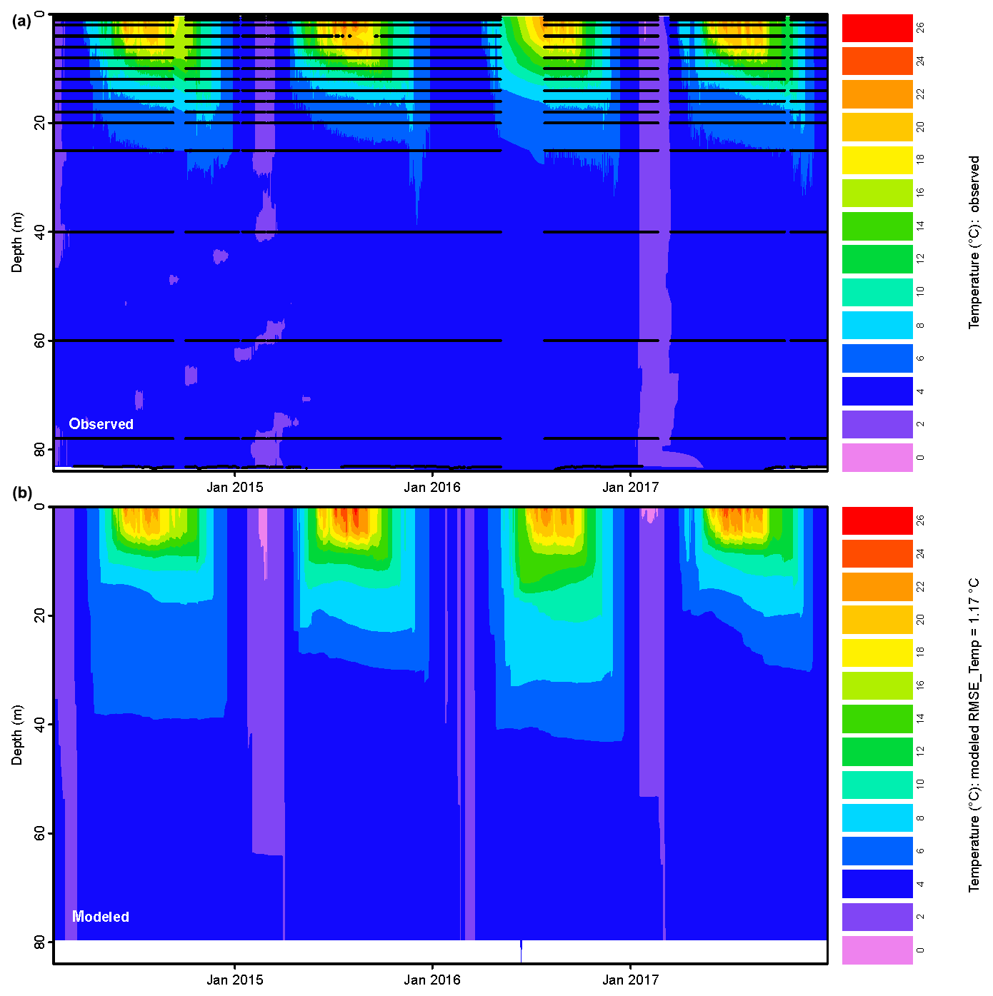
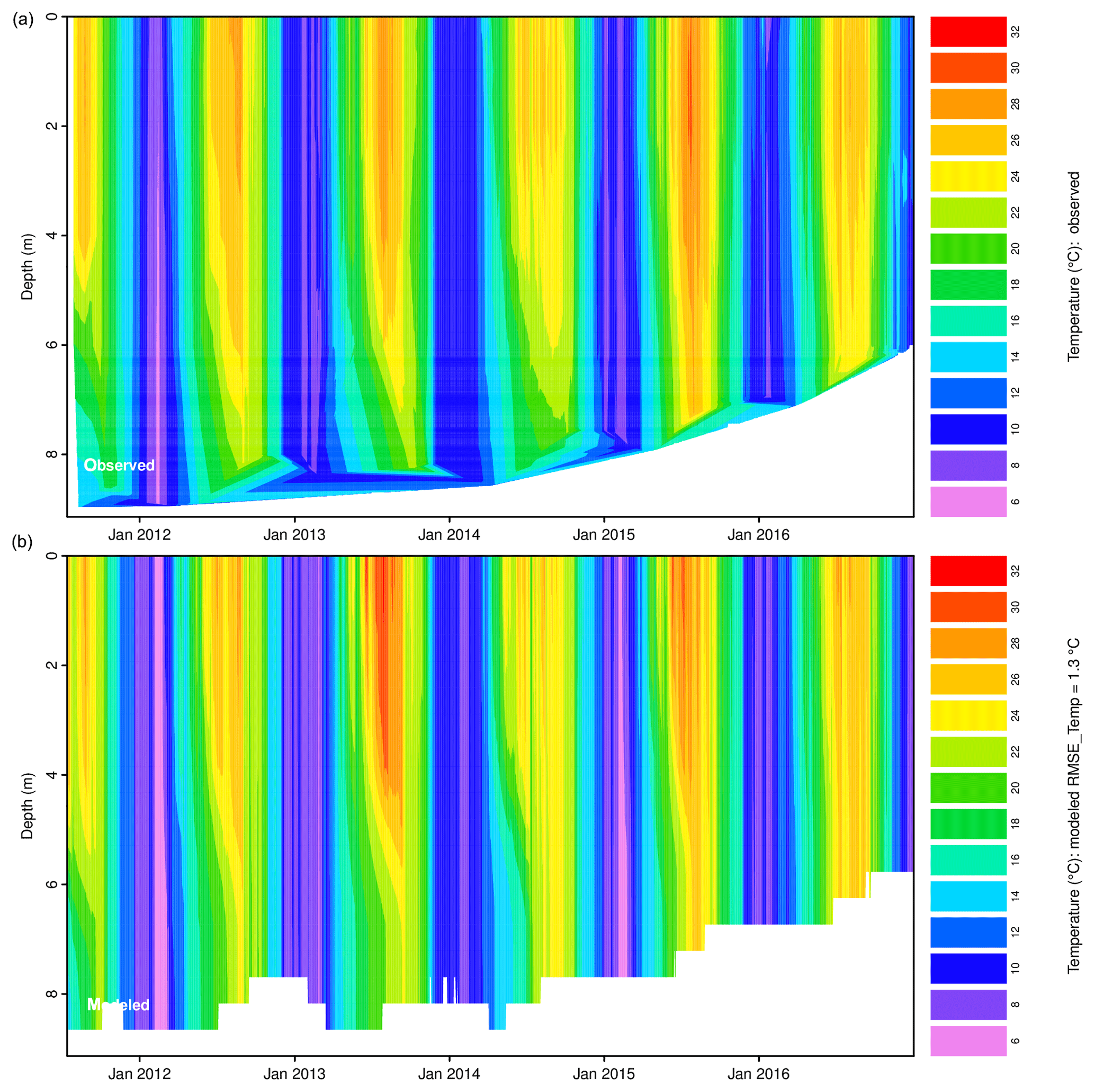
Figure 2Example of a contour plot of observed (a) and modeled (b) water temperatures for lake Ammersee. Black dots mark the availability (time/date and depth) of observed water temperatures.
2.3.3 Sensitivity analysis
To reduce the effort of the model calibration process only sensitive parameters should be included (Luo et al., 2018), which are usually identified by applying a sensitivity analysis. It investigates how variations in the output of a numerical model can be attributed to variations of input parameters or factors (Pianosi et al., 2016). The widely used approach after Lenhart et al. (2002) is implemented in the GUI. The sensitivity index (SI) is calculated for each selected parameter separately, since only one parameter is changed at a time:
The parameter with the value x0 is increased and decreased by Δx. The resulting outputs y1 and y2 (either water temperature, lake level, or the respective RMSEs) are subtracted and normalized by the output y0, which results from using the unchanged parameter value x0; Δx can be set to four different values in the GUI (5 %, 10 %, 20 %, 50 %). It can be chosen out of four grades of relative changes of a parameter. The sensitivity of the simulation can be analyzed with regards to the model output of water temperature or lake level. SI values can be calculated based on either the respective model output or the RMSE, as also applied by Rigosi et al. (2011).
2.3.4 Autocalibration
Since the GLM uses empirical equations (Hipsey et al., 2017), model parameters can be adjusted during the calibration process to minimize the error between model output and observations (Luo et al., 2018). As an alternative to adjusting the parameters manually in the glm2.nml file, glmGUI provides an automatic calibration tool for preselected parameters of surface dynamics, mixing parameters, and hydrological and meteorological factors (Table A2). The user can choose those parameters that are to be included in the calibration process, and they can define a percentage range by which the upper and lower limits of every parameter can be changed from the value in the glm2.nml file. The resolution of the increase or decrease of the parameters within the defined limits can be set as well. According to these settings, model runs of GLM are executed with all possible combinations of the selected parameters (“brute-force”). The overall RMSE of the lake level or water temperature is calculated and saved for every parameter combination to a csv file, with the “best fit” being indicated.
The automated calibration of the lake level includes also the optimization for the parameter inflow_factor for multiple lake inflows. This enables an approximation to the water balance and the reproduction of the lake level if the contribution of inflows is unknown, which is often the case for groundwater inflows or smaller tributaries.
The runtime of the calibration algorithm (tcal) increases exponentially with the number of parameters (p) to be calibrated (Eq. 2):
with r being the number of tested values for each parameter p, and tGLM and tRMSE being runtimes of the lake model and the calculation of the output RMSE, respectively.
3.1 Study site
Lake Baratz is located in the northwest of Sardinia (Fig. 3), Italy, and it is the only natural lake of the island. The elevation of its bottom is 18.6 m a.s.l., and the lake level suffered significant changes in the last 2 decades with a maximum lake depth of 11 m and a minimum of 3 m (Giadrossich et al., 2015; Niedda et al., 2014). The overflow spillway of the lake is at 32.5 m a.s.l. (Niedda et al., 2014). At this maximum level the lake has a surface of about 0.6 km2 and volume of 5.1×10⁶ km3 (Giadrossich et al., 2015). As lake-overflow events to the sea were extremely rare in the past century, the catchment area is considered to be a closed basin (Niedda and Pirastru, 2013). The lake watershed is about 12 km2 with a maximum elevation of 410 m (Pirastru and Niedda, 2013). The only significant tributary inflowing the lake is in the northeast and drains a subcatchment area of 8.1 km2. Due to a very dry summer season, the water inflow starts usually in December and ends in May (Giadrossich et al., 2015).
The lake can be classified as eutrophic and the water is brackish. Thermal stratification usually establishes in February or early March and lasts until early autumn (Giadrossich et al., 2015). Lake mixing occurs all throughout winter, and thus it can be classified as a warm monomictic lake.
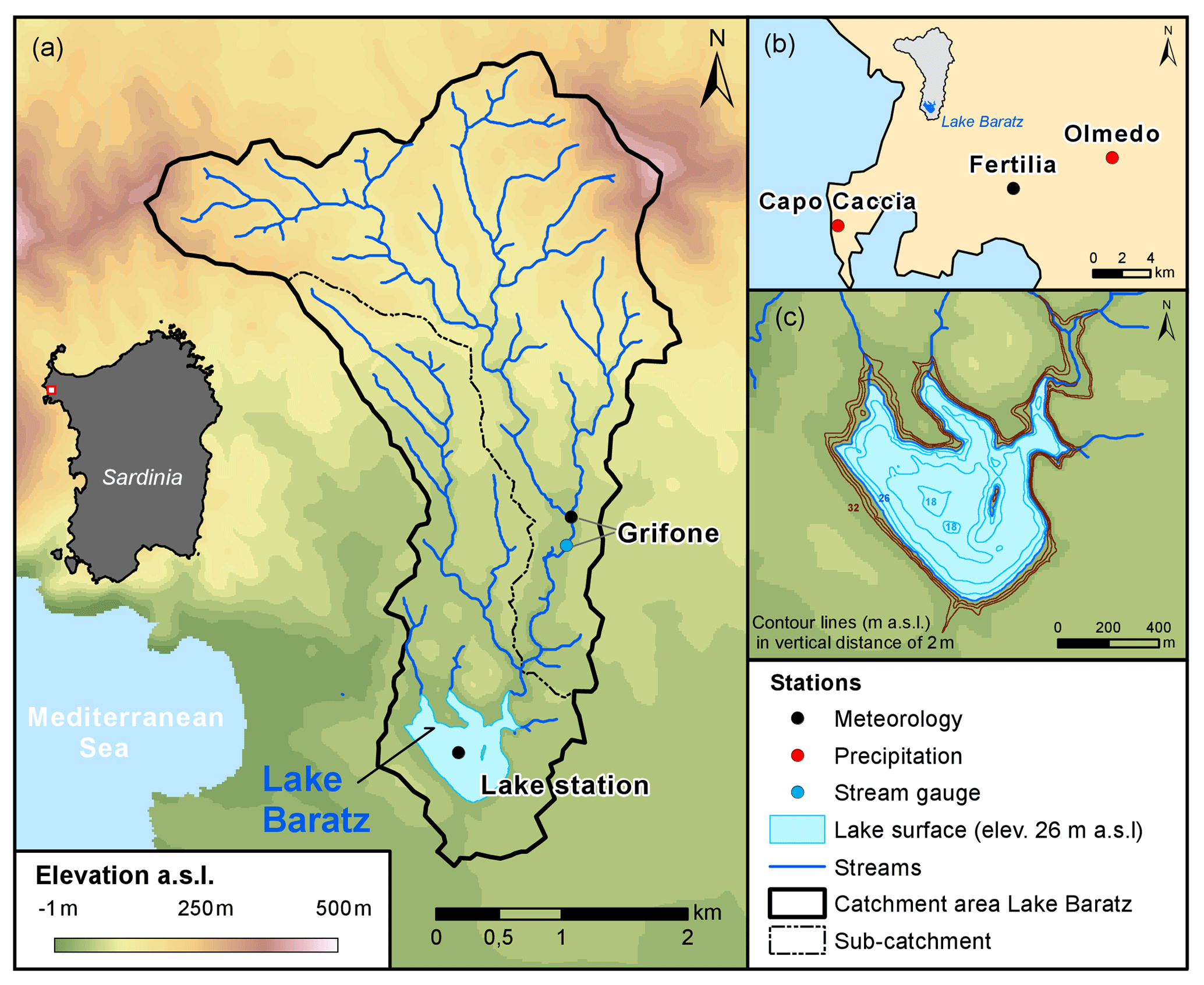
Figure 3(a) Lake Baratz and its hydrological catchment area and observation station; (b) observation stations outside of the lake watershed (gray area); (c) contour lines of the lake basin. The blue area indicates the lake surface at a lake level of 8 m (equal to an elevation of 26 m a.s.l.) observed in November 2012. Brown lines display dry terrain and cyan isobaths at this lake level (Source DEM © Regione Autonoma della Sardegna).
3.2 Sensitivity analysis and calibration
The simulation period for lake Baratz is determined to be 13 July 2011 to 31 December 2016. We assume the light extinction coefficient value, Kw=0.57 m−1, is representative of the whole study period. Kw is calculated by dividing the Secchi-disk constant (in this case the minimum value of 1.44 was taken as it usually ranges between 1.44 and 1.80; Hornung, 2002; Holmes, 1970; Chapra, 2008) by the mean Secchi-disk depth of 2.50 m (data from June 2016 to June 2017). A similar value can be obtained considering a Secchi-disk average depth of 3 m (assumed when the lake had a higher water level) and Secchi-disk constant of 1.70 (Poole and Atkins, 1929). A further detailed description of the applied meteorological and hydrological model input data, the field data, and the data processing can be found in the Supplement.
The calibration process of the lake level was accomplished without hydrological parameters, as preliminary estimations of the water balance considering the seasonality of the inflow and subsurface outflow already exist (see the Supplement Sect. S1.3), which are also applied in this study. Thus, the sensitivity analysis was performed by considering only the parameters of surface dynamics and the wind_factor as wind can have an impact on the lake level due to its influence on evaporation. The options of 10 % increase and the RMSE as a measure of deviation were selected.
After Lenhart et al. (2002), only one of four parameters (cd) is found to have a negligible sensitivity as indicated by a SI value of below 0.01. The analysis revels a high sensitivity for the parameters ch (SI =0.234, see also Fig. 4) and ce (SI =0.334) and a medium sensitivity for wind_factor (SI =0.089).
The sensitivity analysis regarding water temperature was conducted for parameters of lake mixing, surface dynamics, and the wind_factor with the same options as selected for the lake level. Negligible SI values of 0.005 and below are found for all considered parameters, except for ce (SI =0.232) and wind_factor (0.290) with high sensitivities and ch (0.050) with a sensitivity at the threshold between medium and small (Fig. 4). According to both sensitivity analyses, the model is calibrated first for the lake level considering these three parameters with medium and high sensitivities. As the model is found to be sensitive to lake level and water temperature simulations for changes in the same parameters, the calibration for water temperature simulations was performed only considering ce and wind_factor to prevent a decline of the lake level reproduction by the water temperature calibration. Not considering parameter ch is plausible, as its SI value only matches just the threshold to be medium sensitive. In addition, small parameter value ranges of 10 % are applied. Within the calibration process, a total number of approx. 3000 simulation runs were conducted in 6 autocalibration runs.
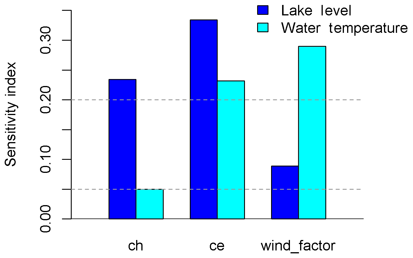
Figure 4Sensitivity index (SI) after Lenhart et al. (2002) of GLM simulations of lake Baratz regarding the lake level (blue) and water temperature (cyan). The lower horizontal line (SI =0.05) marks the threshold between small and medium sensitivity and the upper line (SI =0.20) between medium and high sensitivity.
3.3 Simulation results
The calibration processes for lake-level simulations of the lake model reveal the best fit when applying an unchanged parameter value for ch, an adjustment of ce to 0.001748, and an adjustment of wind_factor to 1.56. The simulated lake level of lake Baratz shows very good model fit criteria with an average RMSE =0.11 m and an average MBE =0.05 m. The seasonal pattern of the lake level, characterized by a strong increase during winter and a drop during summer, is represented well. Additionally, the general decrease of the water stage by about 3 m during the simulation period is simulated correctly, which proves the capability of the model to reproduce the water balance of the lake and its catchment area.
The modeled water temperatures simulated with the adapted lake parameters found by the (auto)calibration yield an overall average RMSE of 1.30 ∘C. A period of remarkable deviation of simulated and observed lake level is induced in January 2014, which could be attributed to uncertainties in the discharge input data simulated by a hydrological model. The basin in that period of the year is still in an intermediate status of soil moisture. Probably the hydrological model overestimated the discharge on the base of rainfall events in January 2014, which in reality did not produce a significant lake-level variation (see Fig. 2 in Giadrossich et al., 2015). However, the observed and simulated lake levels in Fig. 5 have the same trend, and the error caused in January is propagated throughout the year.
The model reproduces stratified and isothermal conditions (Fig. 6). A detailed overview on the temporal and spatial differences between the observed and simulated water temperatures is given in Fig. B1. The simulation can be assessed as a robust fit (Bruce et al., 2018), especially when considering the high degree of thermal dynamics due to the shallow depth of the lake and an additional enhancement by highly variable lake level (Fig. 6). The results also approve GLM to be applicable for shallow lakes in warm climates with a high variety in lake level.
4.1 Study site
The pre-alpine lake Ammersee (Fig. 7) has a maximum depth of 83.7 m (Fig. S8, the Supplement), a surface area of 46.6 km2, and a volume of about 1.8×10⁹ km3 (Bueche and Vetter, 2014b). The mixing regime can be classified as dimictic, but also monomictic seasons occur (Bueche, 2016). The trophic status is currently mesotrophic (Vetter and Sousa, 2012).
The lake has a catchment area of about 994 km2, and its outflow is in the north (Stegen gauge station). The main tributary is river Ammer, which contributes approximately 80 % to the total annual discharge to the lake (Bueche and Vetter, 2015). Several other streams and creeks inflow into the lake, but only the rivers Rott and Fischbach have a share of greater than 5 % of the total lake catchment area size (see Fig. 7). Additionally, groundwater is assumed to inflow to the lake, which has not been quantified yet (Bueche and Vetter, 2014a). The mean lake level is 532.9 m a.s.l. and usually varies about 1 m (Bay. LfU, 2018).
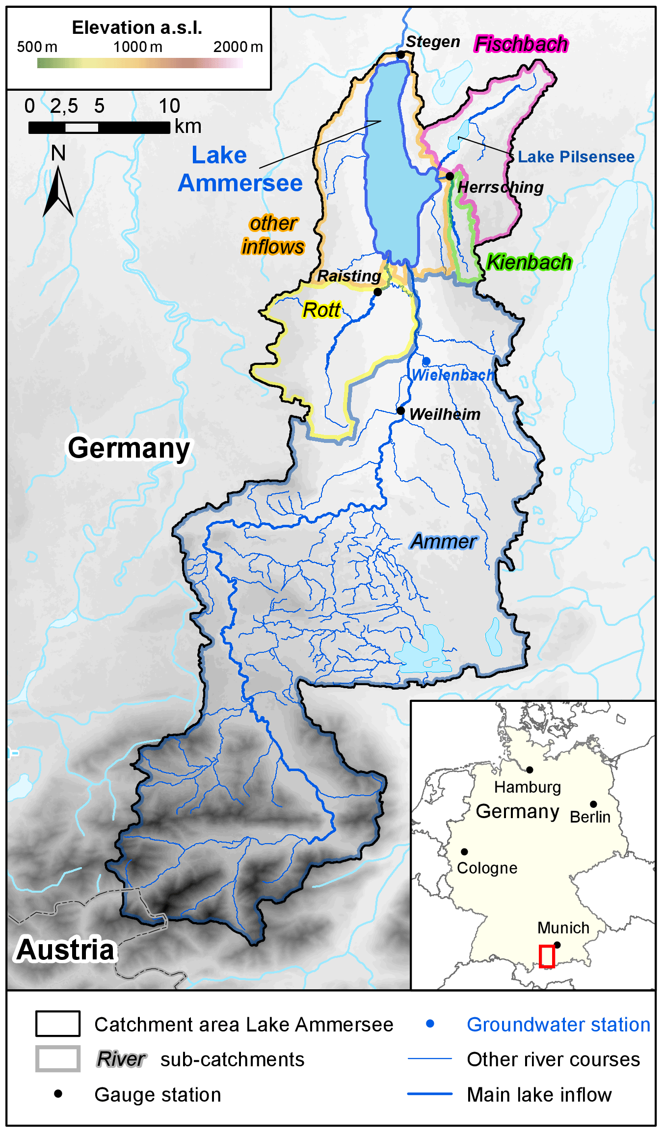
Figure 7Catchment area (with subcatchments) of lake Ammersee. Dots mark the locations of hydrological observation stations (Source DEM: elevation data from ASTER GDEM, a product of METI and NASA; Source geodata: Geobasisdaten © Bayerische Vermessungsverwaltung, http://www.geodaten.bayern.de, last access: 30 January 2020).
4.2 Sensitivity analysis and calibration
The simulation period for lake Ammersee was chosen to be 30 January 2014 to 31 December 2017, starting when reliable field data of the lake station are available consistently (see the Supplement Sect. S2). The initial profile of water temperatures is taken from the observations of that date. No water quality data were available for the simulation period, and the salinity values are derived from conductivity measurements of January 2004, when similar thermal conditions of a slight inverse stratification prevailed and equivalent salinity conditions can be assumed. As the trophic status has not changed since 2004, the average Kw value of 0.35 m−1, determined for the period 2004 to 2008 from Secchi-disk observations (data surveyed and provided by Bavarian Environment Agency), is used for the GLM simulations in this study.
The calibration of the lake level considers the inflow_factor (i.e., simple factor for the discharge values of the inflows) of the four defined inflows of river Ammer; river Fischbach; groundwater inflow; and the sum of river Rott, river Kienbach, and all other unknown inflows. Thus, the adjustment of the representative inflow_factor includes the required correction of the available discharge data, considering the observations are not taken at the stream inlet to the lake but at an upstream location. This is especially relevant for river Ammer with its gauge at Weilheim (Fig. 7). Meteorological input data are taken by a raft station at the lake center, except for precipitation and cloud cover data (see the Supplement, Sect. S2, for a detailed description about the sources of the used meteorological and hydrological input data and the processing of the data).
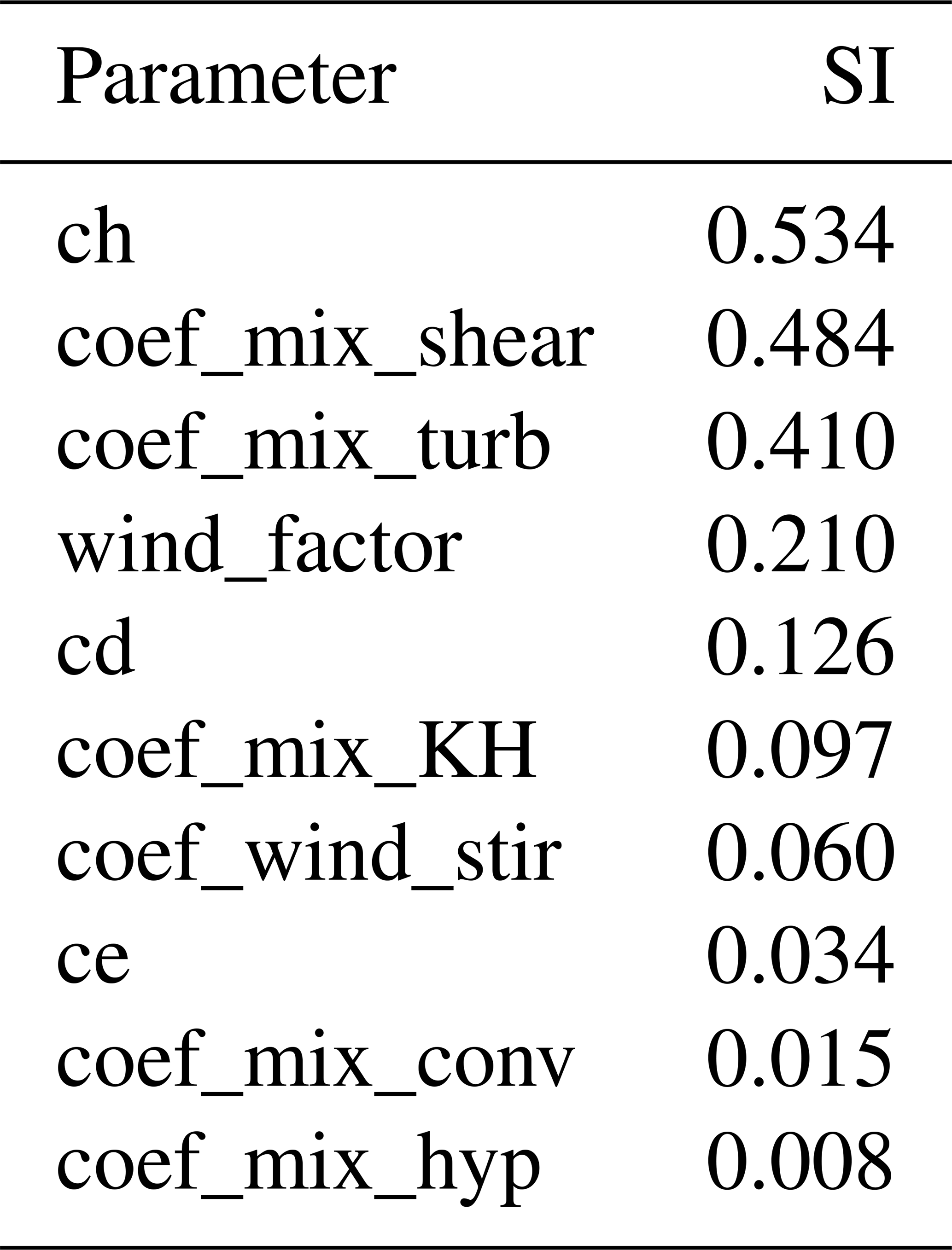
The sensitivity analysis regarding the water temperature (increase: 10 %; measure of difference: RMSE) reveals seven parameters with an SI >0.05, indicating a medium sensitivity (after Lenhart et al., 2002, Table 1). In order to reduce the calculation time of the autocalibration runs, four parameters of high sensitivity with a SI above 0.2 are chosen for this process. In total approx. 50 000 simulation runs in 12 autocalibration runs were performed within the calibration process.
Table 1Values of sensitivity index (SI) for lake Ammersee water temperature simulations.
4.3 Simulation results
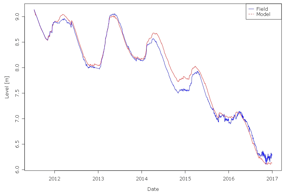
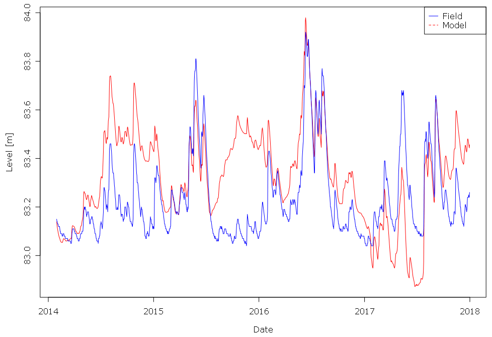
The calibration of the lake-level simulation yields its best fit for the combination of inflow factors for the defined tributaries: river Ammer of 1.10; river Fischbach of 0.72; groundwater of 1.07; and rivers Rott, Kienbach, and all other smaller and unknown inflows of 1.01. By using these adapted inflow factors instead of the default value of 1.0, overall RMSE reduced significantly from 1.10 to 0.20 m, the MBE changed from −1.00 to 0.09 m, and the achieved model fit can be assessed as very satisfactory. The simulation shows periods of general deviations of over 0.20 up to 0.55 m for some months, but it reproduces the short-term fluctuations well (Fig. 8). The remaining errors and differences can be ascribed to the uncertainties and lack of data for some inflows as assumptions and estimations for the unknown surface input and the groundwater inflow had to be made. More detailed hydrological data might explain remarkable dates, like during summer when the trend of simulated and observed lake level changes abruptly. No obvious explanation for these trend shifts could be found, although a detailed investigation of the existing hydrological data was conducted. An impact of a highly complex groundwater inflow system is likely to have a key role in the water balance of the lake, which is not considered by the applied input data sufficiently. Furthermore it cannot be ruled out that unknown alterations or errors in the observation setup of the gauges cause these “turning points” as some of them correspond to flood events, which might have implied problems with the measurements. However, it was possible to improve the lake-level simulation distinctively by considering only the parameter inflow_factor for multiple inflows within the calibration process.
Simulated water temperatures reveal an overall RMSE of 1.172 ∘C. The highest deviations occur within the metalimnion at a depth between 7 and 18 m (Bueche and Vetter, 2014b) during summer stratification, when the model underestimates the temperature (Fig. 9). This is accompanied by layers that are too warm in the upper epilimnion at a depth of about 20 m. However, the general seasonal pattern is reproduced adequately, and differences during winter are negligible.

Figure 9Contour plot of differences between simulated and observed water temperatures of lake Ammersee.
The implemented option of an autocalibration in the toolbox enables a less time-consuming and more efficient parameter optimization compared to a conventional manual calibration procedure (Luo et al., 2018). The utilization of such automatization techniques is advised for lake modeling studies (Ladwig et al., 2018). Hence, the provided tool can be seen as the centerpiece of the developed GLM toolbox, which is complemented by the plotting option of differences between observed and simulated water temperatures. This model output visualization enables an immediate overview on the simulated deviations and their spatial distribution without any further postprocessing of the model results. Although no detailed quantification of the error is possible, this illustration allows for a very quick qualitative comparison of different simulation settings. Such a visualization option for GLM output has not yet been provided for an open-source software.
The easy handling and free availability of the GUI expands the reach of the GLM to potential users beyond limnological research specialists. The used scripting language R is already widespread in limnological (e.g., Winslow et al., 2016), hydrological, and environmental research (e.g., Pilz et al., 2017; Gampe et al., 2016), as well as in the field of automation of water management processes (e.g., Erban et al., 2018). Providing the R code as a development version (https://doi.org/10.5281/zenodo.2025865, Wenk et al., 2018) in addition to the R package enables the GUI and its tools to be easily customized by users for other specific demands and to be shared with the public.
Due to the small number of considered parameters in the calibration process of the presented case studies, the efficiency was successfully tested for a realistic effort of time. The visibility of the simulation error provided by the difference contour plots provides an opportunity to combine the automated calibration easily with expert knowledge. However, the time consumption of an autocalibration run of several days and more for combinations of larger number of parameters and higher intervals might hamper of the calibration efficiency of a solely automatized calibration and can be improved in upcoming versions of the toolbox. At present running the tool on a server in advance or as a “background task” can compensate for this problem.
Further limitations of the toolbox and GUI have to be mentioned and more coding activities should be addressed to minimize the following issues. (1) The contour plots of water temperatures indicate the lake level on the bottom either interpolated or in very coarse lake-level fluctuation, which does not allow for a sufficient derivation of this model output by these plots. For this purpose, separated plots of the lake-level simulations can be created. (2) The calibration algorithm of the toolbox creates parameter values with a high decimal precision due to the approach of percental alteration. This might assume a false sensitivity of the model and a too detailed accuracy of the calibration for the respective parameter. (3) The method of the sensitivity analysis will yield a SI =0 for any included parameter with the initial value being 0. This applies, for example, to seepage_rate as its default value is 0. (4) The applied model version of GLM is dependent on the maintenance of the R package glmtools.
The presented simulations of lake water temperatures have average overall RMSEs of 1.30 and 1.17 ∘C for lake Ammersee and lake Baratz, respectively. This is within the range of values obtained by other lake modeling studies applying GLM or other 1-D lake models (Bueche et al., 2017; Ladwig et al., 2018; Robertson et al., 2018; Frassl et al., 2018). This simulation quality was achieved even by only a few autocalibration runs showing the effectiveness of the tool.
In addition to the visualization options and the calibration tool for water temperature simulations, glmGUI also enables a calibration of the lake level to achieve a correct reproduction of the water stage. This is especially important for smaller lakes, for which an incorrect simulation of the lake level can have a significant impact on the water temperature reproduction. Furthermore, as the lake level is the result of the lake–catchment water balance (Vanderkelen et al., 2018), the applicability of GLM is also enhanced for hydrological analysis and water balance investigations by this feature. The GLM uses the bulk aerodynamic formula to estimate the latent heat flux and therefore evaporation (Hipsey et al., 2014), which is commonly applied to assess the evaporation rate over open water bodies (Fischer et al., 1979; Hicks, 1972). Including the GLM in the hydrological analysis can therefore improve the accuracy of the modeled evaporation, and thus the water balance estimate. In this study, a RMSE for the lake-level simulations of 0.11 m (lake Baratz) and 0.20 m (lake Ammersee) is achieved, which is within the range of the GLM performance shown by Weber et al. (2017), and this attests a good accordance of the modeled water level with the observed values (Hostetler, 1990).
The GUI is also able to execute simulation runs of GLM coupled with water quality models of ecological lake models (e.g., Aquatic Ecodynamics modeling library, AED). Although water quality settings cannot yet be changed using the toolbox, any model-generated output can be plotted.
The presented R package glmGUI combines simulation and processing tools for the GLM. This includes a tool to autocalibrate the model and options for a parameter sensitivity analysis. Both tools can be used to examine the two simulation output variables of water temperature and lake level. Furthermore, glmGUI implements several visualization options for the meteorological and hydrological input data and the model output. After the deployment of other R packages to execute GLM, and for model output post-processing and statistical analysis (rLakeAnalyzer, rGLM, glmtools), glmGUI fills the gap of missing tools to simplify and accelerate the calibration process and to extend visualization options.
The tools are tested for two different lake types (deep, dimictic, perennial inflow and shallow, monomictic, seasonal inflow) located in varying climate zones. Good model results were achieved after a low expenditure of calibration effort. In contrast to many other studies, an exhaustive description of the simulation input data and field data (data for lake Ammersee also provided as example data) is given within this paper (in the Supplement). The GUI includes tools to check the quality of the input data. This comprises the option of a visual detection of errors, missing values, and plausibility.
The development of glmGUI for the free and open-source programming language R, available on all common platforms (Windows, macOS, Linux), makes it accessible for anyone to use, which contributes to scientific transparency (Winslow et al., 2018). The GUI allows for a high level of interoperability due to the option of combining with other operating systems. This includes the coupling of GLM with ecological lake models (e.g., Snortheim et al., 2017; Robertson et al., 2018; Weber et al., 2017; Fenocchi et al., 2019), as the toolbox is already applicable for this purpose and can be the basis for establishing a coupling interface. Furthermore, we designed the software with the aim of a high flexibility for the application of other scenarios, for various study areas, or with diverse time steps. An increasing number of lake modeling studies are investigating the impact of global change on lakes using as meteorological input data regional climate model output or future scenarios (Fenocchi et al., 2018; Weinberger and Vetter, 2014; Bueche and Vetter, 2015; Ladwig et al., 2018; Pietikäinen et al., 2018; Piccolroaz and Toffolon, 2018). For analyses in these fields of research, the presented R package glmGUI will be a powerful tool, especially concerning the provided difference contour plots.
Table A1Required model input data (after Hipsey et al., 2014).
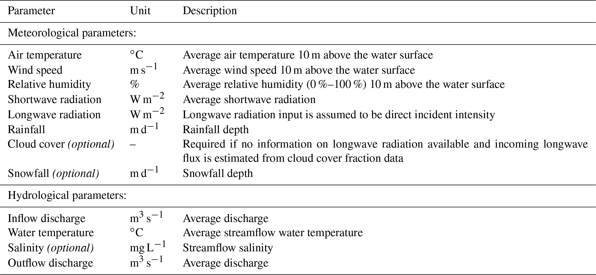
Table A2List of preselected parameters for autocalibration (after Hipsey et al., 2017).
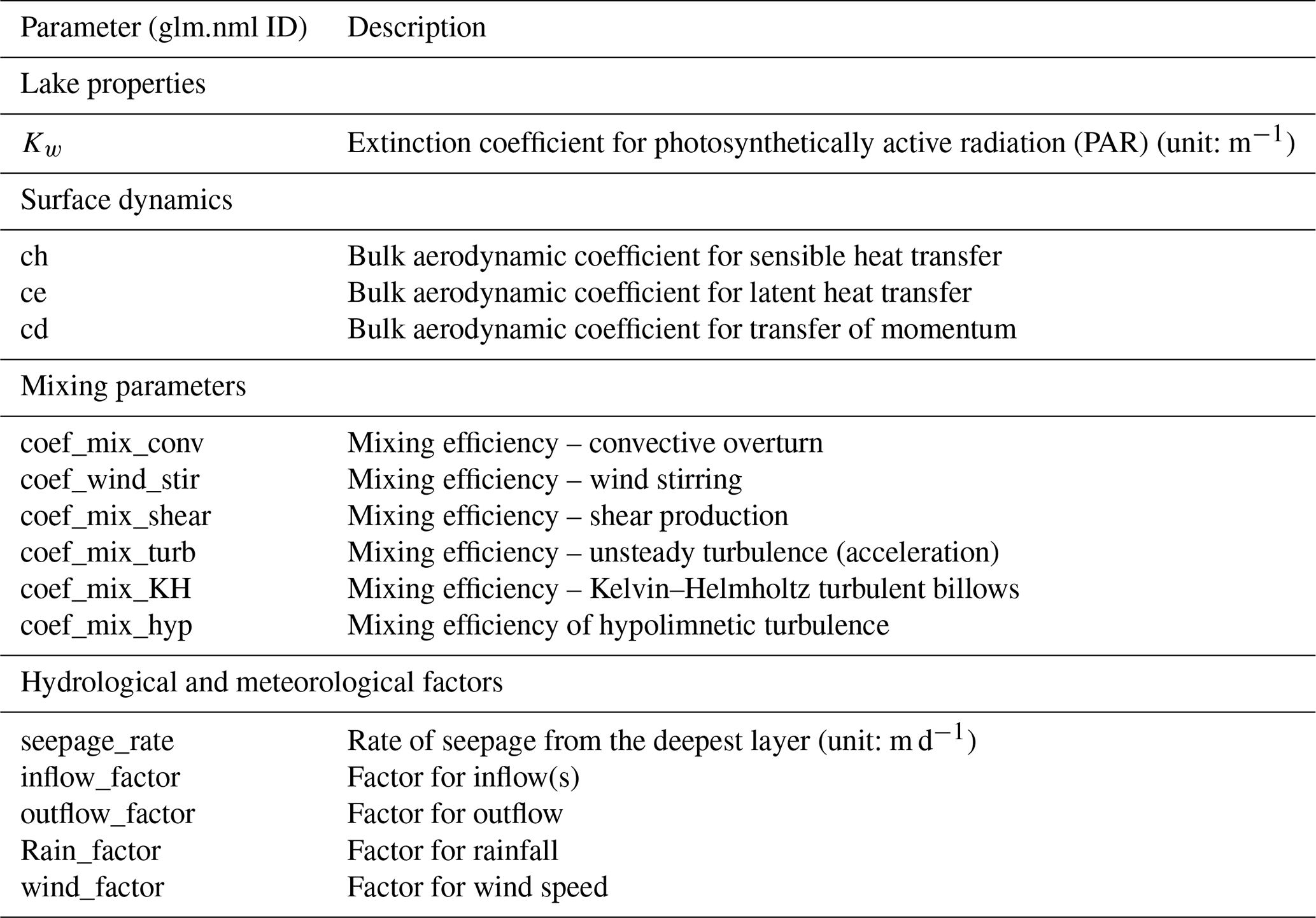
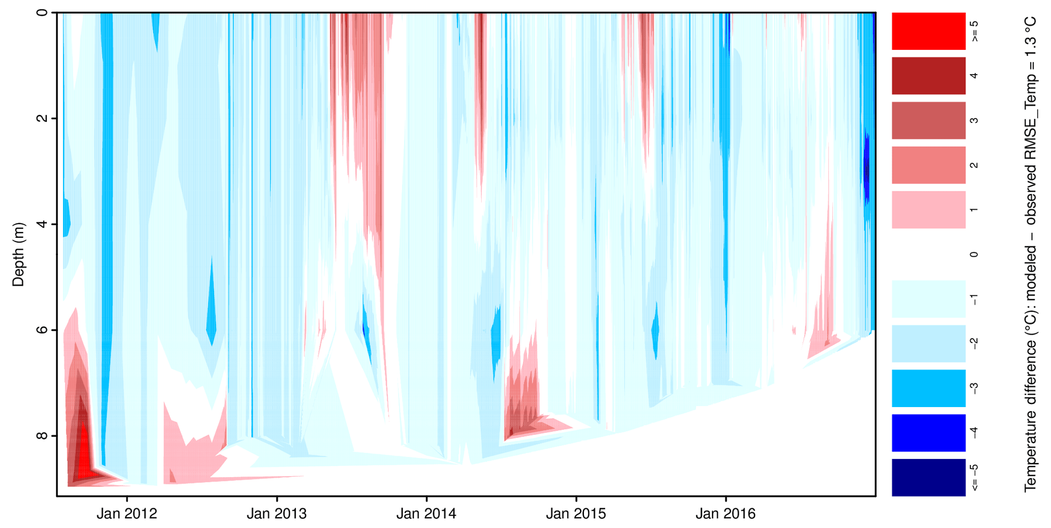
Figure B1Contour plot of differences between simulated and observed water temperatures of lake Baratz.
The package and R code are available at https://doi.org/10.5281/zenodo.2025865 (Wenk et al., 2018). Example data for lake Ammersee are attached to this paper in the Supplement. Sources are described in the Supplement Sect. S2.
The supplement related to this article is available online at: https://doi.org/10.5194/gmd-13-565-2020-supplement.
TB and MV initiated the idea and concept of glmGUI. MW and BP developed the glmGUI package and code. The study sites were suggested by TB and FG. FG and MP operated the raft station and data collection at lake Baratz. Data preprocessing was conducted by TB with the support of MP, FG, and BP. Simulations and analyses have been conducted by TB with the support of FG, MP, and MV. The article was prepared by TB with contributions from all co-authors.
The authors declare that they have no conflict of interest.
We are grateful to the University of Sassari for funding 1 month of professorship for Thomas Bueche in Sassari. We are thankful for the financial support for this study by the teaching and research program Lehre@LMU, sponsored by the German Federal Ministry of Education and Research (BMBF) (grant no. 01PL17016) and by the mentoring program of LMU Munich. We also thank Bachisio Padedda for providing ecological data observations of lake Baratz and Helge Olberding for assisting work. Finally, we pay a silent tribute to Marcello Niedda, who initiated and expedited the hydrological investigations at lake Baratz.
The University of Applied Sciences Würzburg-Schweinfurt supported the publication of this research.
This paper was edited by Steve Easterbrook and reviewed by three anonymous referees.
Bay. LfU (Bayerisches Landesamt für Umwelt): Gewässerkundlicher Dienst Bayern, available at: https://www.gkd.bayern.de/ (last access: 30 January 2020), 2018.
Bruce, L. C., Frassl, M. A., Arhonditsis, G. B., Gal, G., Hamilton, D. P., Hanson, P. C., Hetherington, A. L., Melack, J. M., Read, J. S., Rinke, K., Rigosi, A., Trolle, D., Winslow, L., Adrian, R., Ayala, A. I., Bocaniov, S. A., Boehrer, B., Boon, C., Brookes, J. D., Bueche, T., Busch, B. D., Copetti, D., Cortés, A., de Eyto, E., Elliott, J. A., Gallina, N., Gilboa, Y., Guyennon, N., Huang, L., Kerimoglu, O., Lenters, J. D., MacIntyre, S., Makler-Pick, V., McBride, C. G., Moreira, S., Özkundakci, D., Pilotti, M., Rueda, F. J., Rusak, J. A., Samal, N. R., Schmid, M., Shatwell, T., Snorthheim, C., Soulignac, F., Valerio, G., van der Linden, L., Vetter, M., Vinçon-Leite, B., Wang, J., Weber, M., Wickramaratne, C., Woolway, R. I., Yao, H., and Hipsey, M. R.: A multi-lake comparative analysis of the General Lake Model (GLM): Stress-testing across a global observatory network, Environ. Modell. Softw., 102, 274–291, https://doi.org/10.1016/j.envsoft.2017.11.016, 2018.
Bucak, T., Trolle, D., Tavşanoğlu, Ü. N., Çakıroğlu, A. İ., Özen, A., Jeppesen, E., and Beklioğlu, M.: Modeling the effects of climatic and land use changes on phytoplankton and water quality of the largest Turkish freshwater lake: Lake Beyşehir, Sci. Total Environ., 621, 802–816, https://doi.org/10.1016/j.scitotenv.2017.11.258, 2018.
Bueche, T.: The mixing regime of Lake Ammersee, Erde, 147, 275–283, https://doi.org/10.12854/erde-147-24, 2016.
Bueche, T. and Vetter, M.: Influence of groundwater inflow on water temperature simulations of Lake Ammersee using a one-dimensional hydrodynamic lake model, Erdkunde, 68, 19–31, https://doi.org/10.3112/erdkunde.2014.01.03, 2014a.
Bueche, T. and Vetter, M.: Simulating water temperatures and stratification of a pre-alpine lake with a hydrodynamic model: calibration and sensitivity analysis of climatic input parameters, Hydrol. Process., 28, 1450–1464, https://doi.org/10.1002/hyp.9687, 2014b.
Bueche, T. and Vetter, M.: Future alterations of thermal characteristics in a medium-sized lake simulated by coupling a regional climate model with a lake model, Clim. Dynam., 44, 371–384, https://doi.org/10.1007/s00382-014-2259-5, 2015.
Bueche, T., Hamilton, D. P., and Vetter, M.: Using the General Lake Model (GLM) to simulate water temperatures and ice cover of a medium-sized lake: a case study of Lake Ammersee, Germany, Environ. Earth Sci., 76, 461–475, https://doi.org/10.1007/s12665-017-6790-7, 2017.
Carey, C. C. and Gougis, R. D.: Simulation modeling of lakes in undergraduate and graduate classrooms increases comprehension of climate change concepts and experience with computational tools, J. Sci. Educ. Technol., 26, 1–11, 2017.
Chapra, S. C.: Surface water-quality modeling, Waveland press, 2008.
Erban, L. E., Balogh, S. B., Campbell, D. E., and Walker, H. A.: An R Package for Open, Reproducible Analysis of Urban Water Systems, With Application to Chicago, Open Water Journal, 5, 26–40, 2018.
Fenocchi, A., Rogora, M., Sibilla, S., and Dresti, C.: Relevance of inflows on the thermodynamic structure and on the modeling of a deep subalpine lake (Lake Maggiore, Northern Italy/Southern Switzerland), Limnologica, 63, 42–56, https://doi.org/10.1016/j.limno.2017.01.006, 2017.
Fenocchi, A., Rogora, M., Sibilla, S., Ciampittiello, M., and Dresti, C.: Forecasting the evolution in the mixing regime of a deep subalpine lake under climate change scenarios through numerical modelling (Lake Maggiore, Northern Italy/Southern Switzerland), Clim. Dynam., 51, 3521–3536, 2018.
Fenocchi, A., Rogora, M., Morabito, G., Marchetto, A., Sibilla, S., and Dresti, C.: Applicability of a one-dimensional coupled ecological-hydrodynamic numerical model to future projections in a very deep large lake (Lake Maggiore, Northern Italy/Southern Switzerland), Ecol. Model., 392, 38–51, https://doi.org/10.1016/j.ecolmodel.2018.11.005, 2019.
Fischer, H. B., List, J. E., Koh, C. R., Imberger, J., and Brooks, N. H.: Mixing in Inland and Coastal Waters, Academic Press, 1979.
Frassl, M., Weber, M., and Bruce, L. C.: The General Lake Model (GLM), NETLAKE toolbox for the analysis of high-frequency data from lakes (Factsheet 3), Technical report. NETLAKE COST Action ES1201, 11–15, 2016.
Frassl, M., Boehrer, B., Holtermann, P., Hu, W., Klingbeil, K., Peng, Z., Zhu, J., and Rinke, K.: Opportunities and Limits of Using Meteorological Reanalysis Data for Simulating Seasonal to Sub-Daily Water Temperature Dynamics in a Large Shallow Lake, Water, 10, 594, https://doi.org/10.3390/w10050594, 2018.
Gampe, D., Ludwig, R., Qahman, K., and Afifi, S.: Applying the Triangle Method for the parameterization of irrigated areas as input for spatially distributed hydrological modeling – Assessing future drought risk in the Gaza Strip (Palestine), Sci. Total Environ., 543, 877–888, https://doi.org/10.1016/j.scitotenv.2015.07.098, 2016.
Giadrossich, F., Niedda, M., Cohen, D., and Pirastru, M.: Evaporation in a Mediterranean environment by energy budget and Penman methods, Lake Baratz, Sardinia, Italy, Hydrol. Earth Syst. Sci., 19, 2451–2468, https://doi.org/10.5194/hess-19-2451-2015, 2015.
Grewal, M. S.: Kalman filtering, in: International Encyclopedia of Statistical Science, Springer, 705–708, 2011.
Hanson, P. C., Weathers, K. C., and Kratz, T. K.: Networked lake science: how the Global Lake Ecological Observatory Network (GLEON) works to understand, predict, and communicate lake ecosystem response to global change, Inland Waters, 6, 543–554, 2016.
Hicks, B.: Some evaluations of drag and bulk transfer coefficients over water bodies of different sizes, Bound.-Lay. Meteorol., 3, 201–213, 1972.
Hipsey, M. R., Bruce, L. C., and Hamilton, D. P.: GLM – General Lake Model: Model overview and user information, AED Report #26, The University of Western Australia Technical Manual, 1–42, 2014.
Hipsey, M. R., Bruce, L. C., Boon, C., Busch, B., Carey, C. C., Hamilton, D. P., Hanson, P. C., Read, J. S., de Sousa, E., Weber, M., and Winslow, L. A.: A General Lake Model (GLM2.4) for linking with high-frequency sensor datafrom the Global Lake Ecological Observatory Network (GLEON), Geosci. Model Dev. Discuss., https://doi.org/10.5194/gmd-2017-257, 2017.
Hipsey, M. R., Bruce, L. C., Boon, C., Busch, B., Carey, C. C., Hamilton, D. P., Hanson, P. C., Read, J. S., de Sousa, E., Weber, M., and Winslow, L. A.: A General Lake Model (GLM 3.0) for linking with high-frequency sensor data from the Global Lake Ecological Observatory Network (GLEON), Geosci. Model Dev., 12, 473–523, https://doi.org/10.5194/gmd-12-473-2019, 2019.
Holmes, R. W.: The Secchi Disk in turbid Costal Waters, Limnol. Oceanogr., 15, 688–694, 1970.
Hornung, R.: Numerical Modelling of Stratification in Lake Constance with the 1-D hydrodynamic model DYRESM, University of Stuttgart, Stuttgart, 101 pp., 2002.
Hostetler, S. W.: Simulation of Lake Evaporation With Aoolication to Modeling Lake Level Variations of Harney-Malheur Lake, Oregon, Water Resour. Res., 26, 2603–2612, 1990.
Hyndman, R. J. and Khandakar, Y.: Automatic time series for forecasting: the forecast package for R, 6/07, Monash University, Department of Econometrics and Business Statistics, 2007.
Ladwig, R., Furusato, E., Kirillin, G., Hinkelmann, R., and Hupfer, M.: Climate Change Demands Adaptive Management of Urban Lakes: Model-Based Assessment of Management Scenarios for Lake Tegel (Berlin, Germany), Water, 10, 186, https://doi.org/10.3390/w10020186, 2018.
Lenhart, T., Eckhardt, K., Fohrer, N., and Frede, H.-G.: Comparison of two different approaches of sensitivity analysis, Phys. Chem. Earth, 27, 645–654, 2002.
Luo, L., Hamilton, D., Lan, J., McBride, C., and Trolle, D.: Autocalibration of a one-dimensional hydrodynamic-ecological model (DYRESM 4.0-CAEDYM 3.1) using a Monte Carlo approach: simulations of hypoxic events in a polymictic lake, Geosci. Model Dev., 11, 903–913, https://doi.org/10.5194/gmd-11-903-2018, 2018.
Mi, C., Frassl, M. A., Boehrer, B., and Rinke, K.: Episodic wind events induce persistent shifts in the thermal stratification of a reservoir (Rappbode Reservoir, Germany), Int. Rev. Hydrobiol., 103, 71–82, https://doi.org/10.1002/iroh.201701916, 2018.
Niedda, M. and Pirastru, M.: Hydrological processes of a closed catchment-lake system in a semi-arid Mediterranean environment, Hydrol. Process., 27, 3617–3626, https://doi.org/10.1002/hyp.9478, 2013.
Niedda, M., Pirastru, M., Castellini, M., and Giadrossich, F.: Simulating the hydrological response of a closed catchment-lake system to recent climate and land-use changes in semi-arid Mediterranean environment, J. Hydrol., 517, 732–745, https://doi.org/10.1016/j.jhydrol.2014.06.008, 2014.
Pianosi, F., Beven, K., Freer, J., Hall, J. W., Rougier, J., Stephenson, D. B., and Wagener, T.: Sensitivity analysis of environmental models: A systematic review with practical workflow, Environ. Modell. Softw., 79, 214–232, https://doi.org/10.1016/j.envsoft.2016.02.008, 2016.
Piccolroaz, S. and Toffolon, M.: The fate of Lake Baikal: how climate change may alter deep ventilation in the largest lake on Earth, Climatic Change, 150, 181–194, 2018.
Pietikäinen, J.-P., Markkanen, T., Sieck, K., Jacob, D., Korhonen, J., Räisänen, P., Gao, Y., Ahola, J., Korhonen, H., Laaksonen, A., and Kaurola, J.: The regional climate model REMO (v2015) coupled with the 1-D freshwater lake model FLake (v1): Fenno-Scandinavian climate and lakes, Geosci. Model Dev., 11, 1321–1342, https://doi.org/10.5194/gmd-11-1321-2018, 2018.
Pilz, T., Francke, T., and Bronstert, A.: lumpR 2.0.0: an R package facilitating landscape discretisation for hillslope-based hydrological models, Geosci. Model Dev., 10, 3001–3023, https://doi.org/10.5194/gmd-10-3001-2017, 2017.
Pirastru, M. and Niedda, M.: Evaluation of the soil water balance in an alluvial flood plain with a shallow groundwater table, Hydrolog. Sci. J., 58, 898–911, https://doi.org/10.1080/02626667.2013.783216, 2013.
Poole, H. and Atkins, W.: Photo-electric measurements of submarine illumination throughout the year, J. Mar. Biol. Assoc. UK, 16, 297–324, 1929.
Rigosi, A., Marcé, R., Escot, C., and Rueda, F. J.: A calibration strategy for dynamic succession models including several phytoplankton groups, Environ. Modell. Softw., 26, 697–710, https://doi.org/10.1016/j.envsoft.2011.01.007, 2011.
Robertson, D. M., Juckem, P. F., Dantoin, E. D., and Winslow, L. A.: Effects of water level and climate on the hydrodynamics and water quality of Anvil Lake, Wisconsin, a shallow seepage lake, Lake and Reserv. Manage., 34, 211–231, https://doi.org/10.1080/10402381.2017.1412374, 2018.
Snortheim, C. A., Hanson, P. C., McMahon, K. D., Read, J. S., Carey, C. C., and Dugan, H. A.: Meteorological drivers of hypolimnetic anoxia in a eutrophic, north temperate lake, Ecol. Model., 343, 39–53, 2017.
Vanderkelen, I., van Lipzig, N. P. M., and Thiery, W.: Modelling the water balance of Lake Victoria (East Africa) – Part 1: Observational analysis, Hydrol. Earth Syst. Sci., 22, 5509–5525, https://doi.org/10.5194/hess-22-5509-2018, 2018.
Verzani, J.: Examples for gWidgets, R package version gWidgets 0.0-41, available at: https://cran.r-project.org/web/packages/gWidgets/vignettes/gWidgets.pdf (last access: 30 January 2020), 2014.
Vetter, M. and Sousa, A.: Past and current trophic development in Lake Ammersee – Alterations in a normal range or possible signals of climate change?, Fund. Appl. Limnol., 180, 41–57, https://doi.org/10.1127/1863-9135/2012/0123, 2012.
Weber, M., Rinke, K., Hipsey, M. R., and Boehrer, B.: Optimizing withdrawal from drinking water reservoirs to reduce downstream temperature pollution and reservoir hypoxia, J. Environ. Manage., 197, 96–105, https://doi.org/10.1016/j.jenvman.2017.03.020, 2017.
Weinberger, S. and Vetter, M.: Lake heat content and stability variation due to climate change: coupled regional climate model (REMO)-lake model (DYRESM) analysis, J. Limnol., 73, 93–105, https://doi.org/10.4081/jlimnol.2014.668, 2014.
Wenk, M., Poschlod, B., Büche, T., and Vetter, M.: R Package: glmgui (Version 1.0), Zenodo, https://doi.org/10.5281/zenodo.2025865, 2018.
Williamson, C. E., Saros, J. E., and Schindler, D. W.: Sentinels of Change, Science, 323, 887–888, https://doi.org/10.1126/science.1169443, 2009.
Winslow, L., Read, J., Woolway, R. I., Brentrup, J., Leach, T., and Zwart, J.: rLakeAnalyzer: 1.8.3 Standardized methods for calculating common important derived physical features of lakes, https://doi.org/10.5281/zenodo.58411, 2016.
Winslow, L. A., Zwart, J. A., Batt, R. D., Dugan, H. A., Woolway, R. I., Corman, J. R., Hanson, P. C., and Read, J. S.: LakeMetabolizer: an R package for estimating lake metabolism from free-water oxygen using diverse statistical models, Inland Waters, 6, 622–636, https://doi.org/10.1080/iw-6.4.883, 2018.
- Abstract
- Introduction
- Lake model, software description, and toolbox options
- Case study of lake Baratz
- Case study of lake Ammersee
- Discussion
- Conclusions
- Appendix A: Model input data and calibration parameter
- Appendix B: Contour plot of GLM simulations
- Code and data availability
- Author contributions
- Competing interests
- Acknowledgements
- Financial support
- Review statement
- References
- Supplement