Spatial Referencing of Hyperspectral Images for Tracing of Plant Disease Symptoms


1
INRES Plant Diseases and Plant Protection, University of Bonn, 53115 Bonn, Germany
2
Institute for Sugar Beet Research (IFZ), 37079 Göttingen, Germany
*
Author to whom correspondence should be addressed.
J. Imaging 2018, 4(12), 143; https://doi.org/10.3390/jimaging4120143
Submission received: 5 November 2018
/
Revised: 26 November 2018
/
Accepted: 2 December 2018
/
Published: 4 December 2018
(This article belongs to the Special Issue The Future of Hyperspectral Imaging)
Abstract
:The characterization of plant disease symptoms by hyperspectral imaging is often limited by the missing ability to investigate early, still invisible states. Automatically tracing the symptom position on the leaf back in time could be a promising approach to overcome this limitation. Therefore we present a method to spatially reference time series of close range hyperspectral images. Based on reference points, a robust method is presented to derive a suitable transformation model for each observation within a time series experiment. A non-linear 2D polynomial transformation model has been selected to cope with the specific structure and growth processes of wheat leaves. The potential of the method is outlined by an improved labeling procedure for very early symptoms and by extracting spectral characteristics of single symptoms represented by Vegetation Indices over time. The characteristics are extracted for brown rust and septoria tritici blotch on wheat, based on time series observations using a VISNIR (400–1000 nm) hyperspectral camera.
1. Introduction
Hyperspectral images of plants are suitable to assess the health and vitality state of plants [1,2]. Leaf diseases show characteristic symptoms, allowing a hyperspectral characterization of symptom development [1,3]. The spectral dynamic of symptom development during pathogenesis has been described for numerous plant-pathogen systems [4]. Therefore, hyperspectral imaging has been applied on multiple scales from the leaf level via full plants up to the field and landscape scale [5,6,7,8]. Platforms, microscope stands, laboratory systems, high-throughput facilities, as well as Unmanned Aerial Vehicles (UAVs), planes, and satellites are used [5,6,7,9,10].
This publication focuses on tracking leaf diseases of wheat at the leaf scale. Wheat (Triticum aestivum) is the second most cultivated crop worldwide which is threatened by various pathogens infecting root, stem, leaves, and ears [11]. At the leaf scale, a limiting factor is the natural variability in the spatial and temporal development of disease symptoms [12]. The exact position of symptom appearance and dynamics of development are bound to multiple parameters and, to a certain extent, unpredictable [13,14]. Therefore, symptoms of different development steps are present at a certain point in time, hampering the clear extraction of the typical symptom development.
At best, each symptom has to be traced during the different observation days on its own to have a clearer look on the different steps of pathogenesis. Performing this task is extremely labor intensive and in many situations not feasible, e.g., for the early parts of the pathogenesis before expression of a visible symptom. Few studies have focused this task [5,6], but are restricted to the characterization of single symptoms instead of extracting a representative description of the pathogenesis.
A further advantage of spatially referenced hyperspectral time series is the generation of large amounts of training data with high quality annotation for the training of machine learning models [15]. Even very early effects of the disease could be included as positions on the leaves showing symptoms at a later point in time are known. The underlying assumption is that if disease symptoms are visible, the first changes could most probably be recorded by the hyperspectral camera a few days earlier.
Prerequisite for these applications is a common measurement coordinate system for every image, but its generation on leaf scale is challenging due to leaf movements and growing. The spatial assignment of two images is a common task in computer vision and addressed by the terms image matching or image referencing [16,17,18].
In remote sensing a joint spatial reference system for multiple observations is often provided by the data distributor. Images are georeferenced by an automatic process to localize reflectance characteristics and perform multi-temporal analyses based on repetitive observations of a location. Space and airborne images are georeferenced either by ground control points with known coordinates or by additional sensors determining the location and orientation of the sensor platform. Usually Global Navigation Satellite System (GNSS) receiver are combined with Inertial Measurement Systems (IMS) to reach sufficient global accuracy as well as local continuity [19,20]. Ortho-rectified images are generated by projecting the reflectance information obtained from the 3D earth surface on a 2D reference plane using the determined camera models. By this approach, spatial distortion within the images can be removed [20].
However, in close range scenarios with plants, the image referencing relies typically on the image content instead of external sensors as the measured object cannot be assumed to be solid. Therefore the joint coordinate system is a new concept on the leaf scale. Most of the approaches of extracting geometrical features aim at the classification of plant species based on the shape of its leaf or organs [21,22,23] but the generated features can be transferred to the image matching problem. Gupta et al. [24] investigated the growing characteristics of multiple species using a dense grid of ink markers on the leaves. Based on reference points on a separate reference object, camera models have been further determined for the combination of reflectance and 3D surface data of plants [25,26].
Generally, three method groups to establish correspondence between RGB images can be identified: Point approaches [27], area/contour approaches [28,29], and global approaches in pixel [30] or frequency space [31]. The point approaches detect relevant suitable points within the images and describe their local neighborhood by robust descriptors (e.g., Scale-invariant feature transform, SIFT [32]) allowing an assignment of points from different images. Such methods are rarely used for plant leaves (e.g., [27]) but are the standard procedure for RGB image matching for 3D reconstruction. Area and contour approaches at first extract the leaf within the image and perform an assignment based on the shape or texture characteristics of the leaf surface [29]. Yin et al. [33] used chamfer matching to perform the assignment of Arabidopsis leaves based on their shape. Bar-Sinai et al. [28] used a matching of the local graph of leaf veins to investigate the response of the leaf to mechanical stress. An approach for the multi-modal registration of RGB images and thermal images of plants based on extracted silhouettes in both image types has been developed [34]. There, a non-rigid spline model was used to match the silhouettes and generate the data for the detection of diseased plant tissue [35].
These methods for spatial image matching rely on characteristic shapes or textures. In the present case of parts of wheat leaves none of that is informative. In monocot plants the leaf veins are arranged in parallel and provide no intersections to detect. Moreover, the low spatial resolution of hyperspectral images compared to RGB images prevents the extraction of detailed surface texture information. Disease symptoms may be suitable patterns at later time points but are not present at the earlier days. The silhouette of the fixated leaf parts matches approximately a rectangle, especially for larger leaves where the leaf tip is not captured.
To handle this challenge, artificial reference points of white color have been applied on the leaf surface to allow the image referencing within this study. Leaves are fixated to reduce the complexity to a 2D case approximating the leaf surface by a horizontal 2D plane. In such a case, transformations between different image coordinate systems can be performed by 2D transformation like Affine, Similarity, or Polynomial transformation models [36]. The optimal choice depends on the required model flexibility.
We introduce an approach to spatially reference multiple hyperspectral image cubes of time series experiments. These spatially referenced images form a new 4 dimensional data type with two spatial axis (x and y), one spectral axis (), and a fourth temporal axis (t). Within this new data type disease symptoms can easily be traced back in time, even to the point when no symptom is visible for the human eye.
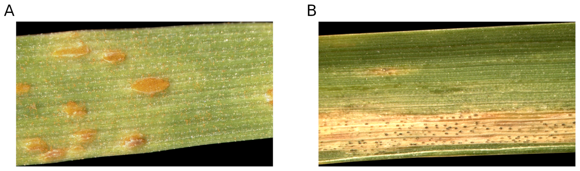
The referencing is performed using an algorithm robust against missing or non-stable reference points by including the RanSaC algorithms [37] and multiple 2D geometric transformations [36] in combination with a well-defined set of control points. As data, time series measurements of wheat leaves fixated in a grid frame assessed by a VISNIR hyperspectral pushbrom camera sensible in the visible (400–680 nm) and near-infrared part of the electro-magnetic spectrum (680–1000 nm) were used. Two relevant diseases of wheat with different symptom expressions were covered: Septoria tritici blotch and brown rust (Figure 1).
2. Materials and Methods
2.1. Plant Material & Fungal Pathogens
2.1.1. Plant Material
Wheat plants (triticum aestivum), cv. Taifun and cv. Chamsin (KWS SAAT SE, Einbeck, Germany) were grown in plastic pots in substrate ED73 (Balster Erdenwerk GmbH, Sinntal-Altengronau, Germany). The plants were grown under greenhouse conditions with 22/20 C day/night temperature, 60 ± 10% RH and a photoperiod of 16 h per day. Plants were inoculated after reaching BBCH growth stage 30 (sprouting) [38].
2.1.2. Fungal Pathogens
Inoculations of wheat plants were done with isolates of Zymoseptoria tritici and Puccinia triticina. The isolate of Z. tritici was cultured on artificial ISP2 media. As obligate biotrophic pathogen, P. triticina was maintained on living plants.
2.2. Hyperspectral Measurements
A hyperspectral line scanning spectrograph (ImSpector V10E, Spectral Imaging Ltd., Oulu, Finland), covering the VISNIR spectral range from 400–1000 nm has been used for image assessment [6]. Images had a spectral resolution of up to 2.8 nm and a spatial resolution of 0.14 mm per pixel. This results in a hyperspectral datacube with 211 bands and 1600 px per image line. A homogeneous illumination was ensured by using six ASD-Pro-Lamps (Analytical Spectral Devices Inc., Boulder, CO, USA). Camera and illumination were installed on a motorized line scanner (Spectral Imaging Ltd.). Camera settings and motor control were adapted using the SpectralCube software (Version 3.62, 2000, Spectral Imaging Ltd.).
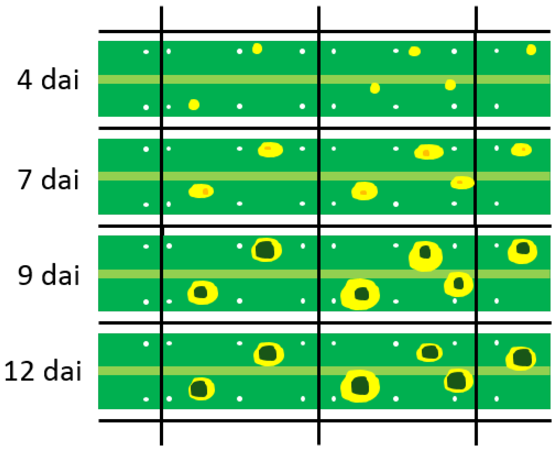
Leaves have been horizontally fixed in a tray using strings allowing imaging of around 20 cm of each leaf. Multiple leaves have been placed side by side within a single image. White color spots are applied as reference points on the leaves to allow image referencing. As shown in Figure 2, six spots in two rows are applied to each leaf section of approximately 4 cm. Observing five leaf sections limited by the fixating strings results in 30 white color spots on each leaf.
As background material, blue cardboard has been selected as it supports background segmentation. For brown rust, time series measurements from 2 to 12 days after inoculation (dai) have been captured. Contrarily, for septoria tritici blotch 15 to 27 dai were covered due to the deviating process of pathogenesis. The data has been normalized, i.e., reflectance was calculated relative to a barium sulphate white reference (Spectral Imaging Ltd.) and a dark current measurement. Normalization has been performed following [39] using ENVI 4.6 + IDL 7.0 (EXELIS Visual Information Solutions, Boulder, CO, USA).
2.3. Algorithm for Hyperspectral Image Referencing
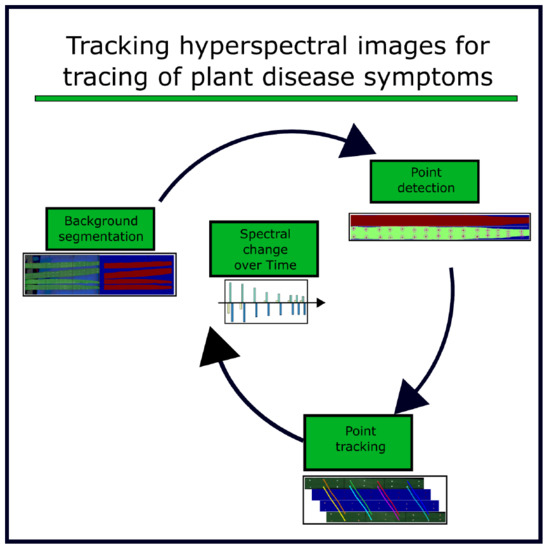
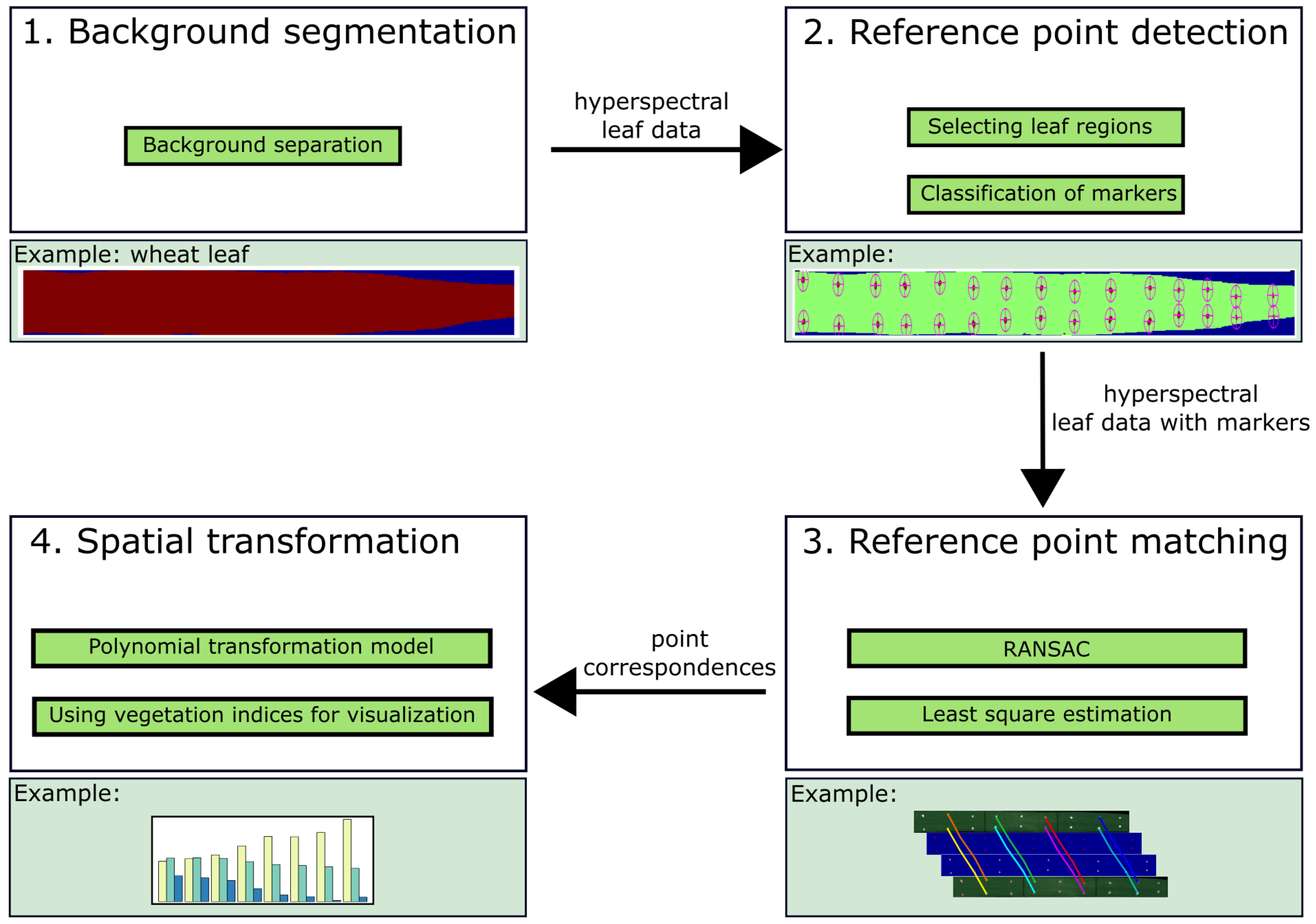
The proposed algorithm is divided into four steps: 1. background segmentation, 2. reference point detection, 3. matching of reference points, and 4. the spatial transformation (Figure 3).
2.3.1. Background Segmentation
The background segmentation relies on the classification method Random Forest algorithm [40] to separate leaf regions and background. The model was trained by manual annotation of a single hyperspectral image. As training data 1000 pixels of the blue background, 1000 pixels of healthy leaf tissue, 1000 pixels of chlorotic leaf tissue, and 500 pixels of spore stocks were randomly sampled from the annotation in which the human expert has tried to represent the class variability. Remaining artifacts of misclassified pixels causing very small regions and holes within large regions were corrected using connected components approach. Leaf regions were extracted and identified by corresponding leaf number based on the position within the image.
2.3.2. Reference Point Extraction
For the selection of the reference points, the Random Forest algorithm was applied as well. By manual annotation 100 pixels of the white reference points and 1000 pixels of plant material (balanced mixture of healthy, chlorotic, and spore stock tissue) were selected and used to train the model. Classified regions within a size range of 3 to 40 pixels were regarded and the center of gravity was extracted as the pixel position. To exclude mixed pixels, the reference point region has been extended by 3 pixel and removed from the leaf regions.
2.3.3. Assignment of Reference Points
Point correspondence was used to derive the geometric transformation model between two images of a leaf recorded at different observation days. Following, the assignment of single reference points between the different observation dates is a prerequisite for image transformation. In our approach, the Random Sample Consensus (RanSaC) algorithm [37] determines a preliminary nonreflective similarity transformation by assigning two random reference points in the base image to two random points in the image to reference. The models were evaluated by projecting each reference point of the origin image to the target image and assess the distance to the closest reference points of the target image. Reference points within a distance of 20 px are assumed to be correct and, therefore, support the model. By repeating this process and selecting the transformation model with the maximum number of supporting reference points, a preliminary referencing was performed. Using nearest neighbor assignment with a distance threshold of 20 px, reference points were assigned and reference points without counterpart were excluded from the further process.
2.3.4. Spatial Image Transformation Models
A transformation model was derived using the corresponding reference points. It is used to reference all images of a time series to the first observation day. The type and flexibility need to be adapted to the specific task. We compared different transformation types [36]: Nonreflective Similarity, Affine, Projective, Polynomial, and Local Weighted Mean (LWM).
Nonreflective Similarity transformation is defined by rotation, translation, and scaling. Adding a shearing parameter and another scale factor results in an Affine transformation. The Projective transformation represents a central-projective transformation between the two image coordinate systems and is defined by eight coefficients [36]. The Polynomial model relates the coordinates within the two images by a mathematical description based on two 2D polynomials. We selected polynomials of order 3 as they are able to represent the assumed leaf movements. The LWM model differs from the mentioned transformation due to its local character. The image is divided into regions in which a local polynomial transformation model is applied [41].
All steps of the algorithm have been performed using Matlab 2013a (The Mathworks, Natick, MA, USA) and the corresponding Image Processing Toolbox.
2.3.5. Evaluation of Transformation Accuracy
Evaluation of the transformation accuracy was performed by the Root Mean Square Error (RMSE) on Euclidean deviations of n reference points
To evaluate the transformation quality, assessing the mean accuracy of projected reference points is not sufficient. Large distortions or missing image information can occur in parts of the leaf without affecting the RMSE parameter. Therefore, two further quality parameters were introduced: Stability and Extrapolation. The first is defined as the RMSE of an inner point, if it is not included into the transformation model. This approximates the transformation quality of arbitrary points of the leaf. The extrapolation parameter approximates the transformation quality at the leaf border by the transformation accuracy of the four outer points point in the first and last point columns at the leaf base and the leaf tip (cv. Figure 2). The evaluation has been performed on the full time series (11 images) of a representative leaf showing brown rust symptoms. For the accuracy measurement , for the extrapolation , and for the stability reference points have been used. The hold out reference points for stability calculation have been evenly distributed within the inner points.
2.4. Vegetation Indices
For characterization of the spectral development of symptomatic areas, Vegetation Indices based on selected spectral bands () have been used. The Normalized Difference Vegetation Index (NDVI) uses a combination of a red band (670 nm) and a NIR band (800 nm) according to formula 2 to extract information about plant vitality and Chlorophyll content [10]. In addition, the Photochemical Reflectance Index (PRI) was calculated, using the difference between two bands in the green color range (531 nm and 570 nm) [42] as well as the Anthocyanin Reflectance Index (ARI) that uses a green (550 nm) and a NIR (700 nm) band which is sensitive to changes in carotenoid pigments [43].
The selected Vegetation Indices are correlated to different plant-physiological parameters (chlorophyll content, photochemical activity, anthocyanin content) which are significantly influenced during disease development.
2.5. Presymptomatic Labeling
To demonstrate the advantages of a fully referenced data set, we used spatial referencing to move the border of symptoms that can be annotated retrospectively regarding the infection time. At first a supervised classification model (Random Forest algorithm [40]) has been derived on the full spectral information based on manual annotations of vital plant material, chlorotic regions, and spore stocks of brown rust (training data composition given in Section 2.3.1). Such models reproduce the visual annotation with good accuracy but are not able to detect invisible effect.
Here, spectra of pixels that were two days later detected as diseased were include in the training data and the Random Forest model is retrained. Furthermore, only pixels were included that are observed at every observation day to guarantee continuous time series observation for every point on the leaf surface within the data set. The extended annotations are used to retrain the classification model.
3. Results
This section presents the obtained results of the spatial referencing algorithm for hyperspectral images and the proposed applications tracing of symptoms and advanced labeling. The referencing approach has been applied to time series observations of two different diseases: Septoria tritici blotch and brown rust, each represented by twelve leaves. Figure 4 shows the effect of referencing by the RGB visualization of hyperspectral images showing a progressing brown rust infection 2–12 dai.
Figure 5 shows the results of tracing mature symptoms back in time. For brown rust and septoria tritici blotch, a continuous transition starting from healthy tissue has been extracted. The final state represents the deviating symptom appearance of the diseases (cv. Figure 1).
3.1. Background Segmentation and Reference Point Detection
Parts of the algorithm are common and well understood steps in many image analysis pipelines. 1. background segmentation and 2. reference point detection did not limit the accuracy or performance of the algorithm. The used Random Forest classifier was trained on manually annotated but representative training data and reached on this data an accuracy of more than 99%. The derived class images “background vs. leaf” and “leaf vs. reference point” showed a high level of concordance with the visual impression. In transfer regions, e.g., the unsharp transition of leaf tissue to the white color of the reference points, a true region boundary is not defined. Consequences are neglectable as the center of gravity of the reference point region showed a high level of reproducibility within the different images.
In contrast, the matching of the reference points to the base image of day 1 is challenging if larger movement had occur or missing points complicate the assignment process. The RanSaC algorithm determines a preliminary non-reflective similarity transformation and allows a nearest neighbor assignment. More flexible transformations tend to degenerated cases assigning multiple reference point to a single base point. Using the RanSaC with 10,000 iteration, an optimum has been found in each case, whereas using only 1000 iteration led to a suboptimal result in around 10% of the runs.
3.2. Transformation Model
The flexibility and robustness of a transformation model type determines the suitability of the model for a specific task. Average quality parameters of the different models for the full time series of a representative leaf of the brown rust data set are given in Table 1.
The extracted quality parameters indicate advantages of using transformation functions with higher flexibility and more model parameters. In each of the three performance parameters accuracy, stability, and extrapolation, the LWM transformations reached the lowest error rates whereas Similarity and Affine transformation obtained the highest error rates.
3.3. Presymptomatic Labeling
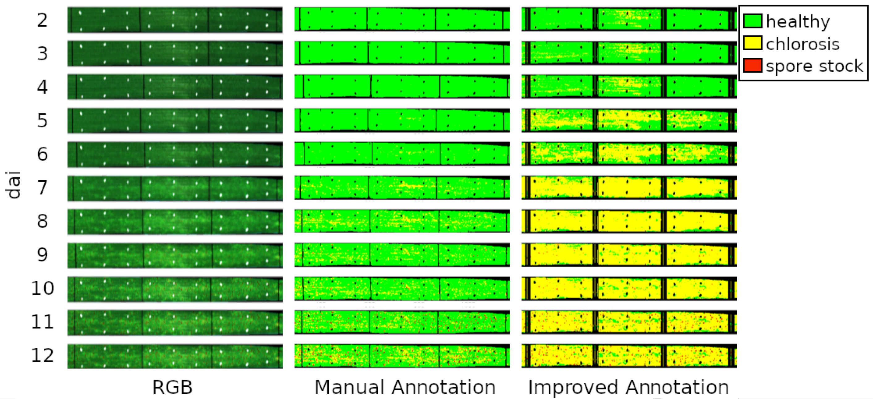
The effect of the extended labeling is shown in Figure 6. The manual annotation allows to detect the spore stocks with good accordance with the visual impression. The highly chlorotic tissue at the later observation data was also selected whereas the transition areas to the vital plant tissue is mostly assigned to the healthy class. The extended labelling allows to move this border between vital and chlorotic tissue. The transition areas are now separated from the vital area and regions showing no visual symptoms are detected.
Non-continuously observed points of the leaf surface were excluded causing that the covered area by the fixation strings are widened as it is summed up for each day.
4. Discussion
The results show that automated referencing of hyperspectral images is possible. The shown approach enables the tracking of spatial symptoms regarding size and reflection in particular for the spectral area between 400–1000 nm. Furthermore, tracking of the spectral characteristics of diseases over time gives new insights for a biological interpretation and an improved detection. This has been shown for brown rust for periods between 2–10 days after inoculation and for 15–30 days for septoria tritici blotch (Figure 5). The time series uncover similarities as well as differences within the type of effect and its dynamics. For both diseases the NDVI is reduced and the ARI increased indicating the degradation of chlorphylls and the production of anthocyanins, but the change by septoria tritici blotch is much sharper. The PRI shows contrary effects if the two disease: Brown rust induces a decrease whereas septoria tritici blotch induces an increase. PRI is related to the photochemical activity meaning the productivity of photosynthesis [42]. This is surprising as the brown rust permits vital leaf tissue whereas septoria tritici blotch causes necrotic tissue. Such response may be explained by the pigments of the produced brown rust spores interfering with the used bands of PRI [44].
The extended labeling showed high potential to train machine learning models with higher sensitivity even in very early symptom stages (Figure 6). To the best of our knowledge, this is a new approach in hyperspectral close range imaging. In non-imaging setups the early symptoms has been classified [45]. In such scenario a spatial referencing is not required, however, this neglects the high sensitivity for small scale symptoms [6].
Conditions for tracing are proper measurement setup and suitable background material allowing a clear background separation. The background material has to differ significantly from the plant material, wilted leaves, reference points, and disease symptoms. The selected blue paper material fulfills these demands. Minor errors occur at reflecting metal edges of the tray but these can be filtered out by a minimal region size. Same applies for the reference points. They need to be durable enough over the experimental period and, furthermore, need to differ significantly from plant material, wilted leaves, and disease symptoms.
Critical parts include the selection of the transformation model as it is always a compromise between robustness and accuracy. The LWM model provides the highest accuracy (Table 1). Nevertheless, the Polynomial transformation model was selected as it reached very similar results compared to the LWM model which tends to produce distorted image areas due to its local character. As local transformation models depend always on a small part of the information, they are less stable but have the ability to represent also local changes due to wilting. In the present data set, the resulting distortions and twisting effects could not be represented by any of the models. Advantages of the local model were therefore very rare whereas negative effects occur much more frequent especially at the leaf borders.
One disadvantage of the showed method is the use of markers on the leaf tissue. Effects of the marker material on the underlying leaf tissue cannot be completely excluded as well as a possible change of the disease development. However, differences were not observed between marked leaves and unmarked control plants.
Limitations for the method are given by the size of the reference points. Using the shortwave-infrared camera (1000–2500 nm; Specim Spectral Imaging Ltd., Oulu, Finland) of the measurement platform, it was not possible to detect them with the required accuracy. The spatial resolution of the shortwave-infrared camera is by a factor of 10 lower than the spatial resolution of the VISNIR camera [25]. Upcoming hyperspectral cameras may be able to allow the spectral referencing also within different spectral regions.
Further research will focus on the use of interest operators on image data as they are used for motion tracking. In particular the use of the SIFT [32] operator for tracking within RGB Image sequences could be an applicable alternative. This could be adapted to the needs of hyperspectral image sequences using different bands and their spectral relation.
Spatial tracking of markers is a key capability for transferring the findings of the shown experiments to the high throughput greenhouse scale (e.g., [46]). Tracking is needed due to leaf movement (external) and plant growth (internal) which leads to a complex transformation of the complete plant. At the moment, the method is limited to 2D leaves due to the integrated geometrical transformations. Even since the data fusion of hyperspectral images and 3D models is possible [25,26], the referencing has many more degrees of freedom. Changes in the shape of the leaf over time has to be represented within the transformation model having the potential to result in a runaway model complexity. Furthermore, reference points within the 3D model has to be selected, described (e.g., by RIFT descriptor [47]), and assigned to image locations. However, extensive studies are required to represent leaf growing and leaf movements by a compact and applicable model. Modelling the complete development of not only geometry, but also nutrient supply and changes in reflectance is possible when using L-Systems [48] or FSP models (FSPM–functional-structural-plant-models) [49] which use substitution in a grammar structure to model the plant development. By this, the continuous geometric referencing of hyperspectral images provides valuable input data for modelling plant growing and development.
5. Conclusions
This publication introduces a method for referencing of hyperspectral images. Field of application is the improved tracking of hyperspectral information of disease symptoms and their development over time. Results have been shown for symptoms and their development of septoria tritici blotch and brown rust, using a VISNIR camera measuring between 400 and 1000 nm. The potential of the method has been demonstrated by extracting the dynamic of spectral indices of a single symptom over time. Furthermore, the possibility to annotate invisible symptoms by tracing visible symptoms back in time to the invisible phase of pathogenesis. The concept of spectral tracking over time can contribute to a more dynamic research of disease development instead of focusing to mature symptoms and their appearing in the visible bands.
Author Contributions
J.B., A.-K.M. and D.B. conceived and designed the experiments; J.B. and D.B. performed the experiments and analyzed the data; J.B., D.B. and S.P. contributed Figures; J.B., S.P., D.B. and A.-K.M. wrote the paper.
Funding
This work was financially supported by BASF Digital Farming.
Acknowledgments
We acknowledge the detailed and constructive remarks of the reviewers.
Conflicts of Interest
The authors declare no conflict of interest.
Abbreviations
| ARI | Anthocyanin Reflectance Index |
| LWM | Local Weighted Mean |
| NDVI | Normalized Difference Vegetation Index |
| PRI | Photochemical Reflectance Index |
| RMSE | Root Mean Square Error |
| UAV | Unmanned Aerial Vehicle |
| VISNIR | Visual-nearinfrared |
References
- Mahlein, A.K.; Kuska, M.; Behmann, J.; Polder, G.; Walter, A. Hyperspectral sensors and imaging technologies in phytopathology: State of the art. Annu. Rev. Phytopathol. 2018, 56, 535–558. [Google Scholar] [CrossRef] [PubMed]
- Blackburn, G.A. Hyperspectral remote sensing of plant pigments. J. Exp. Bot. 2006, 58, 855–867. [Google Scholar] [CrossRef] [PubMed] [Green Version]
- Bock, C.; Poole, G.; Parker, P.; Gottwald, T. Plant disease severity estimated visually, by digital photography and image analysis, and by hyperspectral imaging. Crit. Rev. Plant Sci. 2010, 29, 59–107. [Google Scholar] [CrossRef]
- Mahlein, A.K. Plant disease detection by imaging sensors–parallels and specific demands for precision agriculture and plant phenotyping. Plant Dis. 2016, 100, 241–251. [Google Scholar] [CrossRef]
- Kuska, M.; Wahabzada, M.; Leucker, M.; Dehne, H.W.; Kersting, K.; Oerke, E.C.; Steiner, U.; Mahlein, A.K. Hyperspectral phenotyping on the microscopic scale: Towards automated characterization of plant-pathogen interactions. Plant Methods 2015, 11, 28. [Google Scholar] [CrossRef] [PubMed]
- Mahlein, A.K.; Rumpf, T.; Welke, P.; Dehne, H.W.; Plümer, L.; Steiner, U.; Oerke, E.C. Development of spectral indices for detecting and identifying plant diseases. Remote Sens. Environ. 2013, 128, 21–30. [Google Scholar] [CrossRef]
- Aasen, H.; Burkart, A.; Bolten, A.; Bareth, G. Generating 3D hyperspectral information with lightweight UAV snapshot cameras for vegetation monitoring: From camera calibration to quality assurance. ISPRS J. Photogramm. Remote Sens. 2015, 108, 245–259. [Google Scholar] [CrossRef]
- Honkavaara, E.; Rosnell, T.; Oliveira, R.; Tommaselli, A. Band registration of tuneable frame format hyperspectral UAV imagers in complex scenes. ISPRS J. Photogramm. Remote Sens. 2017, 134, 96–109. [Google Scholar] [CrossRef]
- Burkart, A.; Aasen, H.; Alonso, L.; Menz, G.; Bareth, G.; Rascher, U. Angular dependency of hyperspectral measurements over wheat characterized by a novel UAV based goniometer. Remote Sens. 2015, 7, 725–746. [Google Scholar] [CrossRef] [Green Version]
- Rouse, J., Jr.; Haas, R.; Schell, J.; Deering, D. Monitoring vegetation systems in the Great Plains with ERTS. In Proceedings of the Third Earth Resources Technology Satellite-1 Symposium, Washington, DC, USA, 10–14 December 1973. [Google Scholar]
- Bockus, W.W.; Bowden, R.; Hunger, R.; Murray, T.; Smiley, R. Compendium of Wheat Diseases and Pests, 3rd ed.; American Phytopathological Society (APS Press): Sao Paulo, MN, USA, 2010. [Google Scholar]
- Camargo, A.; Smith, J. An image-processing based algorithm to automatically identify plant disease visual symptoms. Biosyst. Eng. 2009, 102, 9–21. [Google Scholar] [CrossRef]
- West, J.S.; Bravo, C.; Oberti, R.; Lemaire, D.; Moshou, D.; McCartney, H.A. The potential of optical canopy measurement for targeted control of field crop diseases. Annu. Rev. Phytopathol. 2003, 41, 593–614. [Google Scholar] [CrossRef] [PubMed]
- Bravo, C.; Moshou, D.; West, J.; McCartney, A.; Ramon, H. Early Disease Detection in Wheat Fields using Spectral Reflectance. Biosyst. Eng. 2003, 84, 137–145. [Google Scholar] [CrossRef]
- Behmann, J.; Mahlein, A.K.; Rumpf, T.; Römer, C.; Plümer, L. A review of advanced machine learning methods for the detection of biotic stress in precision crop protection. Precis. Agric. 2015, 16, 239–260. [Google Scholar] [CrossRef]
- Hartley, R.; Zisserman, A. Multiple View Geometry in Computer Vision; Cambridge University Press: Cambridge, UK, 2003. [Google Scholar]
- Zitova, B.; Flusser, J. Image registration methods: A survey. Image Vis. Ccomput. 2003, 21, 977–1000. [Google Scholar] [CrossRef]
- Salvi, J.; Matabosch, C.; Fofi, D.; Forest, J. A review of recent range image registration methods with accuracy evaluation. Image Vis. Comput. 2007, 25, 578–596. [Google Scholar] [CrossRef]
- Eling, C.; Klingbeil, L.; Kuhlmann, H. Real-time single-frequency GPS/MEMS-IMU attitude determination of lightweight UAVs. Sensors 2015, 15, 26212–26235. [Google Scholar] [CrossRef] [PubMed]
- Toutin, T. Geometric processing of remote sensing images: Models, algorithms and methods. Int. J. Remote Sens. 2004, 25, 1893–1924. [Google Scholar] [CrossRef]
- Gwo, C.Y.; Wei, C.H. Plant identification through images: Using feature extraction of key points on leaf contours1. Appl. Plant Sci. 2013, 1, 1200005. [Google Scholar] [CrossRef]
- Mouine, S.; Yahiaoui, I.; Verroust-Blondet, A. Combining leaf salient points and leaf contour descriptions for plant species recognition. In Proceedings of the International Conference Image Analysis and Recognition, Povoa do Varzim, Portugal, 26–28 June 2013; Springer: Berlin, Germany, 2013; pp. 205–214. [Google Scholar]
- Kolivand, H.; Fern, B.M.; Rahim, M.S.M.; Sulong, G.; Baker, T.; Tully, D. An expert botanical feature extraction technique based on phenetic features for identifying plant species. PLoS ONE 2018, 13, e0191447. [Google Scholar] [CrossRef]
- Gupta, M.D.; Nath, U. Divergence in patterns of leaf growth polarity is associated with the expression divergence of miR396. Plant Cell 2015. [Google Scholar] [CrossRef]
- Behmann, J.; Mahlein, A.K.; Paulus, S.; Kuhlmann, H.; Oerke, E.C.; Plümer, L. Calibration of hyperspectral close-range pushbroom cameras for plant phenotyping. ISPRS J. Photogramm. Remote Sens. 2015, 106, 172–182. [Google Scholar] [CrossRef]
- Behmann, J.; Mahlein, A.K.; Paulus, S.; Dupuis, J.; Kuhlmann, H.; Oerke, E.C.; Plümer, L. Generation and application of hyperspectral 3D plant models: Methods and challenges. Mach. Vis. Appl. 2016, 27, 611–624. [Google Scholar] [CrossRef]
- De Vylder, J.; Douterloigne, K.; Vandenbussche, F.; Van Der Straeten, D.; Philips, W. A non-rigid registration method for multispectral imaging of plants. In Proceedings of the 2012 SPIE Defense, Security, and Sensing, Baltimore, MD, USA, 23–27 April 2012; Volume 8369, p. 836907. [Google Scholar]
- Bar-Sinai, Y.; Julien, J.D.; Sharon, E.; Armon, S.; Nakayama, N.; Adda-Bedia, M.; Boudaoud, A. Mechanical stress induces remodeling of vascular networks in growing leaves. PLoS Comput. Boil. 2016, 12, e1004819. [Google Scholar] [CrossRef] [PubMed] [Green Version]
- Balduzzi, M.; Binder, B.M.; Bucksch, A.; Chang, C.; Hong, L.; Iyer-Pascuzzi, A.S.; Pradal, C.; Sparks, E.E. Reshaping plant biology: Qualitative and quantitative descriptors for plant morphology. Front. Plant Sci. 2017, 8, 117. [Google Scholar] [CrossRef] [PubMed]
- Wang, X.; Yang, W.; Wheaton, A.; Cooley, N.; Moran, B. Efficient registration of optical and IR images for automatic plant water stress assessment. Comput. Electron. Agric. 2010, 74, 230–237. [Google Scholar] [CrossRef]
- Henke, M.; Junker, A.; Neumann, K.; Altmann, T.; Gladilin, E. Automated alignment of multi-modal plant images using integrative phase correlation approach. Front. Plant Sci. 2018, 9, 1519. [Google Scholar] [CrossRef] [PubMed]
- Lowe, D.G. Distinctive image features from scale-invariant keypoints. Int. J. Comput. Vis. 2004, 60, 91–110. [Google Scholar] [CrossRef]
- Yin, X.; Liu, X.; Chen, J.; Kramer, D.M. Multi-leaf alignment from fluorescence plant images. In Proceedings of the IEEE 2014 IEEE Winter Conference on Applications of Computer Vision (WACV), Steamboat Springs, CO, USA, 24–26 March 2014; pp. 437–444. [Google Scholar]
- Raza, S.E.A.; Sanchez, V.; Prince, G.; Clarkson, J.P.; Rajpoot, N.M. Registration of thermal and visible light images of diseased plants using silhouette extraction in the wavelet domain. Pattern Recognit. 2015, 48, 2119–2128. [Google Scholar] [CrossRef]
- Raza, S.E.A.; Prince, G.; Clarkson, J.P.; Rajpoot, N.M. Automatic detection of diseased tomato plants using thermal and stereo visible light images. PLoS ONE 2015, 10, e0123262. [Google Scholar] [CrossRef]
- Luhmann, T.; Robson, S.; Kyle, S.; Harley, I. Close Range Photogrammetry: Principles, Techniques and Applications; Whittles: Dunbeath, UK, 2006. [Google Scholar]
- Fischler, M.A.; Bolles, R.C. Random sample consensus: A paradigm for model fitting with applications to image analysis and automated cartography. Commun. ACM 1981, 24, 381–395. [Google Scholar] [CrossRef]
- Meier, U. Growth Stages of Mono-and Dicotyledonous Plants; Blackwell, Wissenschafts-Verlag: Berlin, Germany, 1997. [Google Scholar]
- Grahn, H.; Geladi, P. Techniques and Applications of Hyperspectral Image Analysis; John Wiley Sons: Hoboken, NJ, USA, 2007. [Google Scholar]
- Breiman, L. Random forests. Mach. Learn. 2001, 45, 5–32. [Google Scholar] [CrossRef]
- Goshtasby, A. Image registration by local approximation methods. Image Vis. Comput. 1988, 6, 255–261. [Google Scholar] [CrossRef]
- Gamon, J.; Penuelas, J.; Field, C. A narrow-waveband spectral index that tracks diurnal changes in photosynthetic efficiency. Remote Sens. Environ. 1992, 41, 35–44. [Google Scholar] [CrossRef]
- Gitelson, A.A.; Merzlyak, M.N.; Chivkunova, O.B. Optical properties and nondestructive estimation of anthocyanin content in plant leaves. Photochem. Photobiol. 2001, 74, 38. [Google Scholar] [CrossRef]
- Wang, E.; Dong, C.; Park, R.F.; Roberts, T.H. Carotenoid pigments in rust fungi: Extraction, separation, quantification and characterisation. Fungal Boil. Rev. 2018, 32, 166–180. [Google Scholar] [CrossRef]
- Rumpf, T.; Mahlein, A.K.; Steiner, U.; Oerke, E.C.; Dehne, H.W.; Plümer, L. Early detection and classification of plant diseases with Support Vector Machines based on hyperspectral reflectance. Comput. Electron. Agric. 2010, 74, 91–99. [Google Scholar] [CrossRef]
- Kuska, M.T.; Behmann, J.; Grosskinsky, D.K.; Roitsch, T.; Mahlein, A.K. Screening of barley resistance against powdery mildew by simultaneous high-throughput enzyme activity signature profiling and multispectral imaging. Front. Plant Sci. 2018, 9, 1074. [Google Scholar] [CrossRef]
- Lazebnik, S.; Schmid, C.; Ponce, J. A sparse texture representation using local affine regions. IEEE Trans. Pattern Anal. Mach. Intell. 2005, 27, 1265–1278. [Google Scholar] [CrossRef] [PubMed] [Green Version]
- Prusinkiewicz, P.; Lindenmayer, A. The Algorithmic Beauty of Plants; Springer: Berlin/Heidelberg, Germany, 1996. [Google Scholar]
- Vos, J.; Evers, J.B.; Buck-Sorlin, G.H.; Andrieu, B.; Chelle, M.; de Visser, P.H.B. Functional-structural plant modelling: A new versatile tool in crop science. J. Exp. Bot. 2009, 61, 2101–2115. [Google Scholar] [CrossRef] [Green Version]
Figure 1.
RGB images of the symptoms of (A) brown rust caused by Puccinia triticina and (B) septoria tritici blotch caused by Zymoseptoria tritici. Brown rust symptoms are dominated by reddish spore stocks whereas necrotic lesions are characteristic for septoria tritici blotch.
Figure 1.
RGB images of the symptoms of (A) brown rust caused by Puccinia triticina and (B) septoria tritici blotch caused by Zymoseptoria tritici. Brown rust symptoms are dominated by reddish spore stocks whereas necrotic lesions are characteristic for septoria tritici blotch.

Figure 2.
Scheme of the referenced hyperspectral time series of a single leaf observed at four exemplary days. Reference points (white spots), fixating strings (in black), and the developing disease symptoms are included.
Figure 2.
Scheme of the referenced hyperspectral time series of a single leaf observed at four exemplary days. Reference points (white spots), fixating strings (in black), and the developing disease symptoms are included.

Figure 3.
Dataflow of the proposed algorithm for geometric referencing of hyperspectral images.

Figure 4.
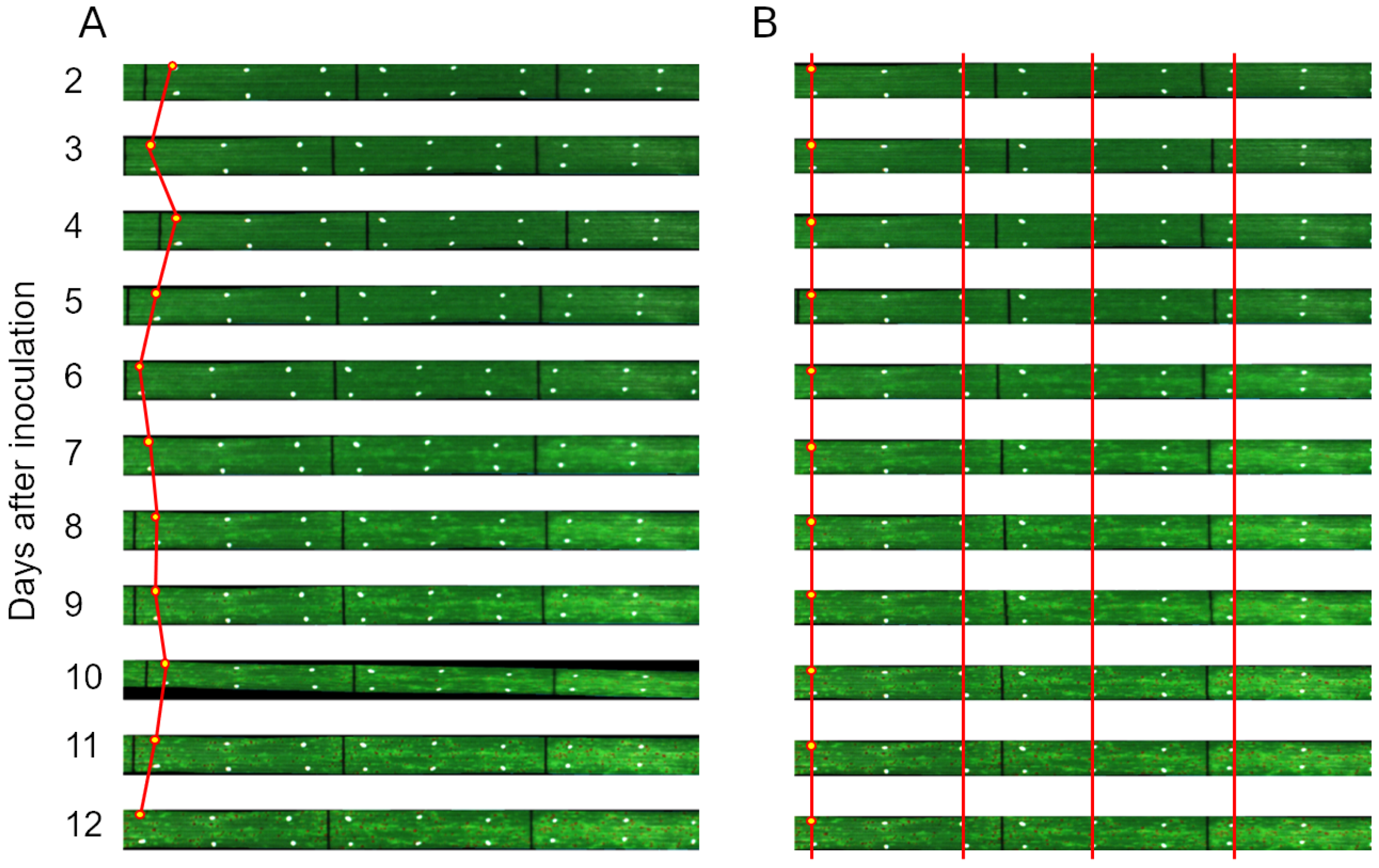
Effect of the spatial referencing. (A) shows the time series of unaligned hyperspectral images and (B) the same time series after the application of the proposed algorithm. To illustrate the result, identical points within the images were connected by red lines.
Figure 4.
Effect of the spatial referencing. (A) shows the time series of unaligned hyperspectral images and (B) the same time series after the application of the proposed algorithm. To illustrate the result, identical points within the images were connected by red lines.

Figure 5.
Visualization of the tracing results by using RGB visualizations of a symptom and the corresponding Vegetation indices anthocyanin reflectance index (ARI), normalized difference vegetation index (NDVI), and photochemical reflectance index (PRI) for brown rust (A,C) and septoria tritici blotch (B,D). For visualization purposes the NDVI was multiplied by 10 and the PRI by 40. Timeseries of spectral characteristics are derived to uncover the deviating spectral dynamics of the diseases.

Figure 6.
RGB visualization and corresponding classification results of a brown rust time series. Compared are the classification results based on a manual annotation and an improved annotation including the data two days before detection.
Figure 6.
RGB visualization and corresponding classification results of a brown rust time series. Compared are the classification results based on a manual annotation and an improved annotation including the data two days before detection.


Table 1.
Performance parameters (accuracy, stability, and extrapolation) of the five transformation model types assessing the suitability for the spatial referencing of wheat leaves. The accuracy is measured by the reprojection error of used reference points. The stability is measured by the reproduction error of unused control points within the leaf and the ability to extrapolate is measured by the root mean square error (RMSE) of unused control points at the base and the tip of the leaf. Displayed are the mean results during the whole time series of eleven days (standard deviation in brackets).
| Similarity | Affine | Projective | Polynomial | LWM | |
|---|---|---|---|---|---|
| Accuracy (px) | 1.24 (0.75) | 1.23 (0.76) | 1.09 (0.75) | 0.26 (0.092) | 0.19 (0.07) |
| Stability (px) | 1.06 (0.62) | 1.08 (0.61) | 0.97 (0.60) | 0.47 (0.17) | 0.36 (0.15) |
| Extrapolation (px) | 2.61 (1.57) | 2.61 (1.59) | 2.37 (1.59) | 0.83 (0.31) | 0.76 (0.30) |
© 2018 by the authors. Licensee MDPI, Basel, Switzerland. This article is an open access article distributed under the terms and conditions of the Creative Commons Attribution (CC BY) license (http://creativecommons.org/licenses/by/4.0/).
Share and Cite
MDPI and ACS Style
Behmann, J.; Bohnenkamp, D.; Paulus, S.; Mahlein, A.-K. Spatial Referencing of Hyperspectral Images for Tracing of Plant Disease Symptoms. J. Imaging 2018, 4, 143. https://doi.org/10.3390/jimaging4120143
AMA Style
Behmann J, Bohnenkamp D, Paulus S, Mahlein A-K. Spatial Referencing of Hyperspectral Images for Tracing of Plant Disease Symptoms. Journal of Imaging. 2018; 4(12):143. https://doi.org/10.3390/jimaging4120143
Chicago/Turabian StyleBehmann, Jan, David Bohnenkamp, Stefan Paulus, and Anne-Katrin Mahlein. 2018. "Spatial Referencing of Hyperspectral Images for Tracing of Plant Disease Symptoms" Journal of Imaging 4, no. 12: 143. https://doi.org/10.3390/jimaging4120143
Note that from the first issue of 2016, this journal uses article numbers instead of page numbers. See further details here.