
A Hybrid DenseNet-LSTM Model for Epileptic Seizure Prediction


Department of Computer Science, Hanyang University, Seoul 40763, Korea
*
Author to whom correspondence should be addressed.
Appl. Sci. 2021, 11(16), 7661; https://doi.org/10.3390/app11167661
Submission received: 20 July 2021
/
Revised: 15 August 2021
/
Accepted: 19 August 2021
/
Published: 20 August 2021
Abstract
:The number of people diagnosed with epilepsy as a common brain disease accounts for about 1% of the world’s total population. Seizure prediction is an important study that can improve the lives of patients with epilepsy, and, in recent years, it has attracted more and more attention. In this paper, we propose a novel hybrid deep learning model that combines a Dense Convolutional Network (DenseNet) and Long Short-Term Memory (LSTM) for epileptic seizure prediction using EEG data. The proposed method first converts the EEG data into the time-frequency domain through Discrete Wavelet Transform (DWT) for use in the input of the model. Then, we train the previously transformed image through a hybrid model combining Densenet and LSTM. To evaluate the performance of the proposed method, experiments are conducted for each preictal length of 5, 10, and 15 min using the CHB-MIT scalp EEG dataset. As a result, we obtained a prediction accuracy of 93.28%, a sensitivity of 92.92%, a specificity of 93.65%, a false positive rate of 0.063 per hour, and an F1-score of 0.923 when the preictal length was 5 min. Finally, as the proposed method is compared to previous studies, it is confirmed that the seizure prediction performance was improved significantly.
1. Introduction
The number of people suffering from epilepsy worldwide is about 50 million. Epilepsy is a neurological brain disorder identified by the frequent occurrence of seizures [1]. Seizures show movement, sensory, cognitive, and behavioral disorders due to the release of abnormal electrical signals from the cerebral cortex. About 30% of patients have incurable epilepsy, whose seizures are not well controlled even with Anti-Epileptic Drugs (AED) [2].
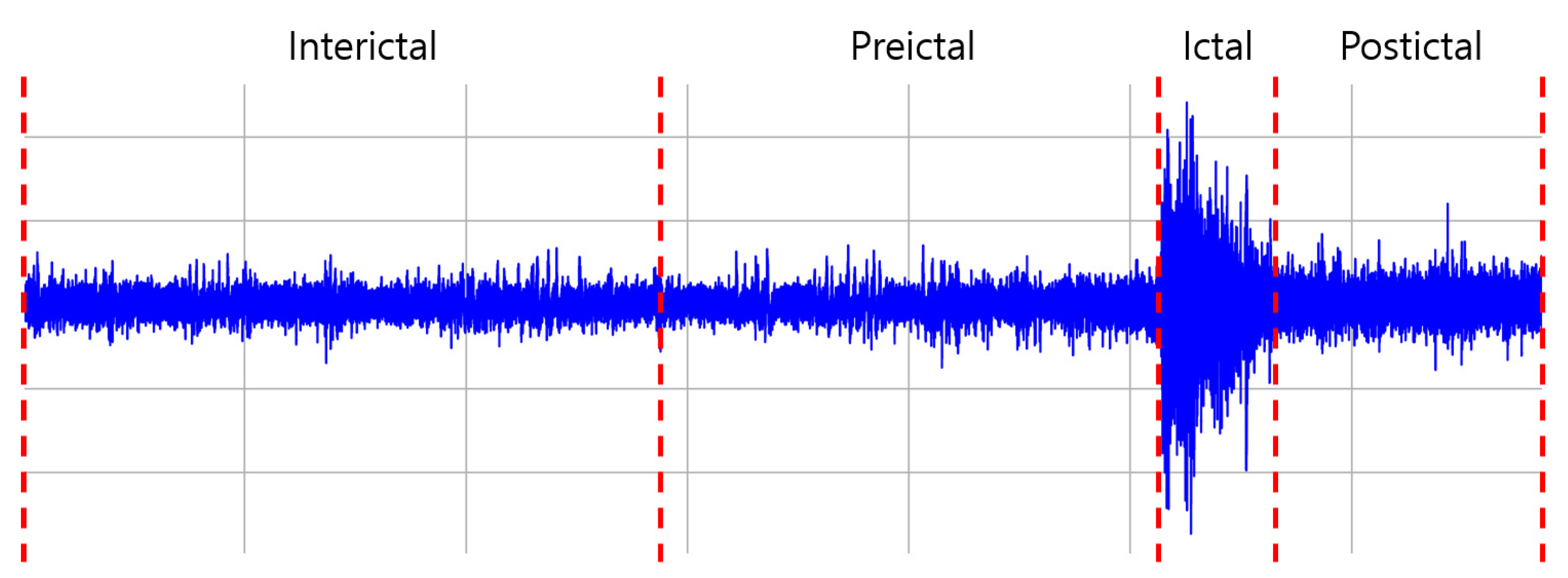
To diagnose and analyze seizures, an electroencephalogram (EEG) is used that records the flow of electricity generated when signals are forwarded between the cranial neurons. EEG can be classified into two types, intracranial EEG and scalp EEG, depending on the location to be measured. An intracranial EEG measures signals by attaching electrodes directly to the cerebral cortex exposed during surgery to record the electrical activity of the cerebral cortex. Scalp EEG measures EEG signals by attaching electrodes to the scalp. Intracranial EEG can obtain signals without noises, but since the skull needs to be incised, the scalp EEG measurement method, which can be used for routine patient monitoring and seizure alarm generation, has higher potential in terms of applicability and ease of use. In addition, according to the EEG record, the EEG state of a seizure patient can be classified into four categories: First, during the onset of a seizure, it is called the ictal. Second, the state before the onset of seizures is called the preictal. Third, the state after the seizure is over is called the postictal. Finally, the interval between seizure and seizure excluding the previously mentioned states is called the interictal [3]. These four states are shown in Figure 1.
Seizures usually occur irregularly, and because it is difficult to predict the exact timing of their occurrence, patients with epilepsy are limited in social activities and are always exposed to the risk of trauma. So, studies on seizure prediction using EEG signals have been conducted steadily to give time to raise an alarm before a seizure onset and take appropriate actions. Seizure prediction begins with the existence of a difference between the interictal and preictal intervals. That is, before the seizure onset, it detects the preictal interval and generates an alarm. In the past few years, machine learning has been widely used in seizure prediction, but in recent years, research using deep learning algorithms that show great performance in fields such as computer vision and speech recognition have mainly been conducted. In seizure prediction, Convolutional Neural Networks (CNN) [4], which are widely used in image processing and show good performances, have attracted the attention of researchers. The supervised learning method using this CNN trains the difference between interictal and preictal states, and the trained classifier predicts the occurrence of seizures by detecting the preictal interval in the new EEG recording.
In this paper, we propose a seizure prediction method using DenseNet-LSTM. Dense Convolutional Network (DenseNet) [5] is an architecture that solves problems such as vanishing gradient or parameter increase that occurs as the CNN layer deepens, and is more advantageous than CNN in training information from limited EEG data. In addition, the Long Short-Term Memory (LSTM) [6] is an architecture that solves the long-term dependence problem of Recurrent Neural Network (RNN) and is mainly used to predict time-series data, so it is suitable for finding temporal features of EEG, which are time-series data. The proposed method consists of two stages. In the first stage, to use the EEG signal as input data of DenseNet, it is converted into image data in the time-frequency domain using Discrete Wavelet Transforms (DWT). In the second stage, seizures are predicted by training the difference between the interictal and preictal states using the EEG signal converted into an image.
The rest of this paper is organized as follows. Section 2 covers previous studies of seizure prediction. Section 3 describes the dataset used, the preprocessing method, and the proposed model. Section 4 presents the performance evaluation according to preictal length and comparative analysis with previous studies. Finally, Section 5 concludes the paper.
2. Related Work
Over the past few years, research in the field of seizure prediction has been ongoing. The basic assumption of seizure prediction is that there is a difference between the interictal and preictal states. In early seizure prediction studies, threshold-based methodology [7,8,9,10,11] or machine learning techniques such as Support Vector Machines (SVM) [12,13,14] were used a lot, but recently, deep learning methods [15,16,17] such as CNN have been studied a lot. Ref. [18] was the first to propose training a deep learning classifier to identify seizures in EEG images, similar to how clinicians identify seizures through visual inspection. Ref. [19] proposed a method of extracting the univariate spectral power of intracranial EEG signals, classifying them through SVM, and removing sporadic and incorrect information using Kalman filters. Their methodology consisted of 80 seizures and 18 patients on the Freiburg dataset, reaching 98.3% sensitivity and 0.29 false positive rate (FPR). Ref. [20] proposed a method of extracting the power spectral density ratio of the EEG signal, further processing it by a second-order Kalman filter, and then inputting it into the SVM classifier for classification. The dataset used for the evaluation is the same as the previous data, reaching 100% sensitivity and 0.03 FPR. Ref. [21] proposed a mechanism for calculating the phase-locking values between the scalp EEG signals and classifying them into interictal and preictal states through SVM using this. Their proposed method was applied to the CHB-MIT dataset consisting of 21 patients and 65 seizures, reaching a sensitivity of 82.44% and a specificity of 82.76%.
In seizure prediction studies using deep learning algorithms, CNN is attracting the most attention. Since seizure prediction studies using CNN usually require data in the form of images as input, the EEG signal is converted into a two-dimensional form through a preprocessing method. The authors of [22] proposed a method of dividing the raw EEG signal by a window size of 30 s, applying Short-Time Fourier Transform (STFT) to extract spectrum information, and then using it as an input to CNN. In the experiment using 64 seizures from 13 patients in the CHB-MIT dataset, reaching a sensitivity of 81.2% and an FPR of 0.16. In [23], an image is transformed into a time-frequency form using Continuous Wavelet Transform (CWT) to see the various frequency bands of EEG. The authors proposed a method of predicting seizures by learning the difference between interictal and preictal states using the transformed data as an input to CNN. The same dataset as before was used, and as a result of testing 18 seizures from 15 patients, the average FPR was 0.142 and was unpredictable for three seizures. In [24], seizure prediction using preprocessed features with spectral band power, statistical moment, and Hjorth parameters as inputs to a multi-frame 3D CNN model is performed, achieving a sensitivity of 85.71% and FPR of 0.096 in the CHB-MIT dataset.
3. Proposed Method: DenseNet-LSTM
3.1. System Model
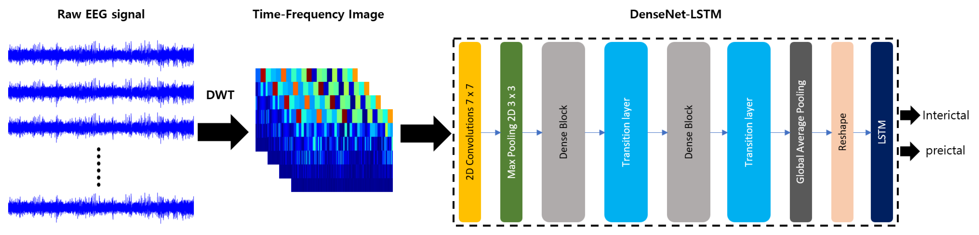
Figure 2 shows the overall system model of the proposed method. First, it goes through a preprocessing method to use the EEG signal as input data to the deep learning model. The preprocessing divides the raw EEG signal by channel and then segments it by the window size and applies the mother function db4 of the DWT to convert it into a time-frequency type 2D image. The db4 is a transform of Daubechies wavelet, it encodes polynomials with two coefficients, which has a relatively fast calculation speed processing time. Next, the preprocessing data are used as the input data of DenseNet, and the resulting feature map is used as the input data of LSTM. As a result, the proposed model trains the difference between interictal and preictal states and then predicts seizures by detecting the preictal state before the onset of seizures.
3.2. Dataset and Preprocessing
3.2.1. Dataset
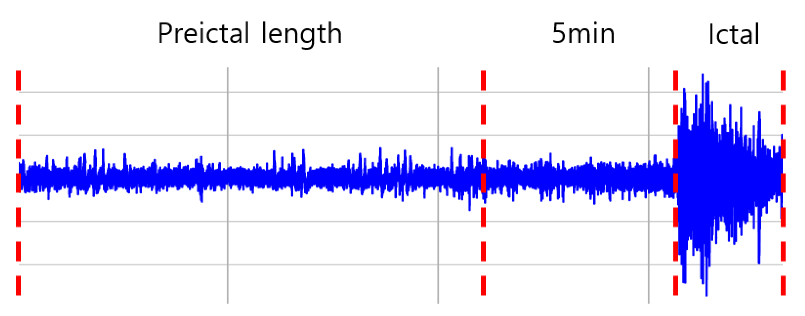
The CHB-MIT dataset used in the paper is a scalp EEG recording measured from 23 pediatric patients at Children’s Hospital Boston, which is a public dataset and is available with open access at PhysioNet.org. This record was measured at a 256 Hz sampling rate using 22 electrodes placed according to the International 10–20 Electrode Positioning System and contains a total of 983 h of consecutive EEG recordings and 198 seizures [25]. As can be seen from the annotation file of the dataset, we can see that the patient’s channel changes frequently. Therefore, we used 18 channels (“FP1-F7”, “F7-T7”, “T7-P7”, “P7-O1”, “FP1-F3”, “F3-C3”, “C3-P3”, “P3-O1”, “FP2-F4”, “F4-C4”, “C4-P4”, “P4-O2”, “FP2-F8”, “F8-T8”, “T8-P8”, “P8-O2”, “FZ-CZ”, “CZ-PZ”) that are commonly used by 24 patients out of a total of 22 electrode channels. Although there are some differences according to the patient’s data, it must be a certain distance from the ictal PHASE to be regarded as interictal. If the distance is too close, seizure waves may be included within the interictal period. Since the distance from the ictal varies from patient to patient, there are two cases considered as interictal. First, patients with close distances used the interictal as far from the ictal as possible. On the other hand, patients with sufficient distance used the interictal at a distance more than a certain distance from the ictal. In addition, we assume the preictal length to be 5, 10, and 15 min because the preictal phase is not clearly distinguished. As shown in Figure 3, there exist the preictal length plus the 5 min interval before the ictal period. Since the model is trained with the preictal data for seizure prediction, the 5 min interval preceding the seizure is excluded from the preictal length purposefully. In real situations, if a seizure can be predicted in advance before the ictal period and the patient can be treated immediately, a certain amount of time (e.g., 5 min) is needed to ensure that the patient has some effect on seizure.
3.2.2. Preprocessing
The raw EEG signal is difficult to analyze because it consists of a time-amplitude domain. So, we use a signal processing method to convert the EEG signal into a time-frequency domain suitable for analysis. Ref. [26] tried to extract spectral information from EEG data which converted to the frequency domain using the Short-Time Fourier Transform (STFT). STFT and Wavelet transform are typical methods of converting a signal into the time-frequency domain. Among them, a wavelet transforms that can reflect a more diverse frequency band was selected by supplementing the shortcomings of STFT. Wavelet transform is a method that can be effectively analyzed in all areas of high frequency or low frequency, and there are CWT and DWT [27].
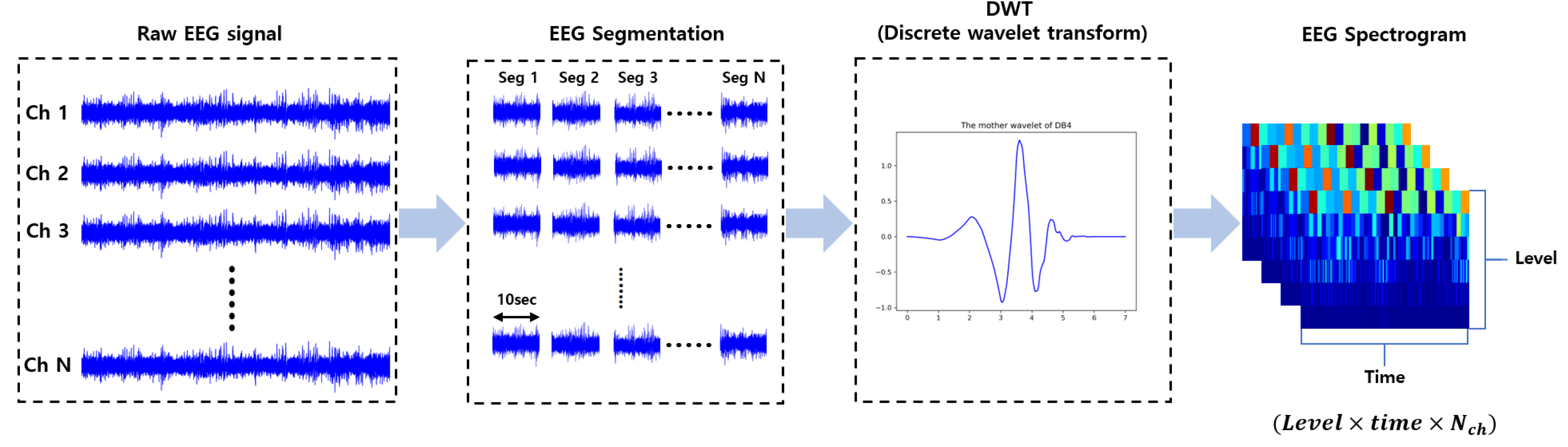
As shown in Figure 4, the original EEG signal is separated for each channel and then segment window size of 10 s. After that, Daubechies 4 (db4) is applied as the mother function of DWT to convert the EEG signal into a two-dimensional image of the time-frequency domain. As an additional parameter, the overlap was set to 1 s, and the frequency level of the DWT was set to 7 (frequency bandwidth in the 2–128 hz section).
3.3. Deep Learning Architecture
3.3.1. DenseNet
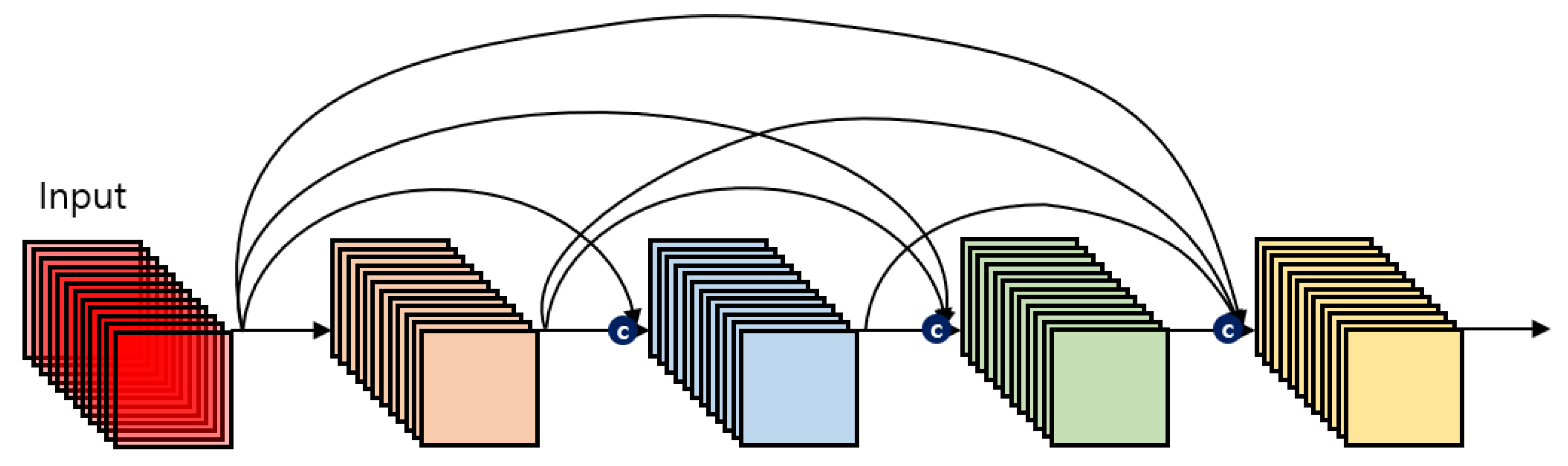
As the network deepens, there is a problem that input or gradient information may vanish when it reaches the end of the network. Various studies are being conducted to solve this problem, and all of them have the feature of making a shortcut from the early layer to the later layer. A densely connected convolutional network, which was introduced at IEEE Conference on Computer Vision and Pattern Recognition (CVPR) in 2017 [5], proposed architecture with great advantages in terms of vanishing gradient, reduced computation, and reduced number of parameters through a new concept of dense connectivity that extends this feature. As shown in Figure 5, dense connectivity is a method of continuously connecting the feature map of the previous layer with the input of the later layer to reinforce the information flow between layers.
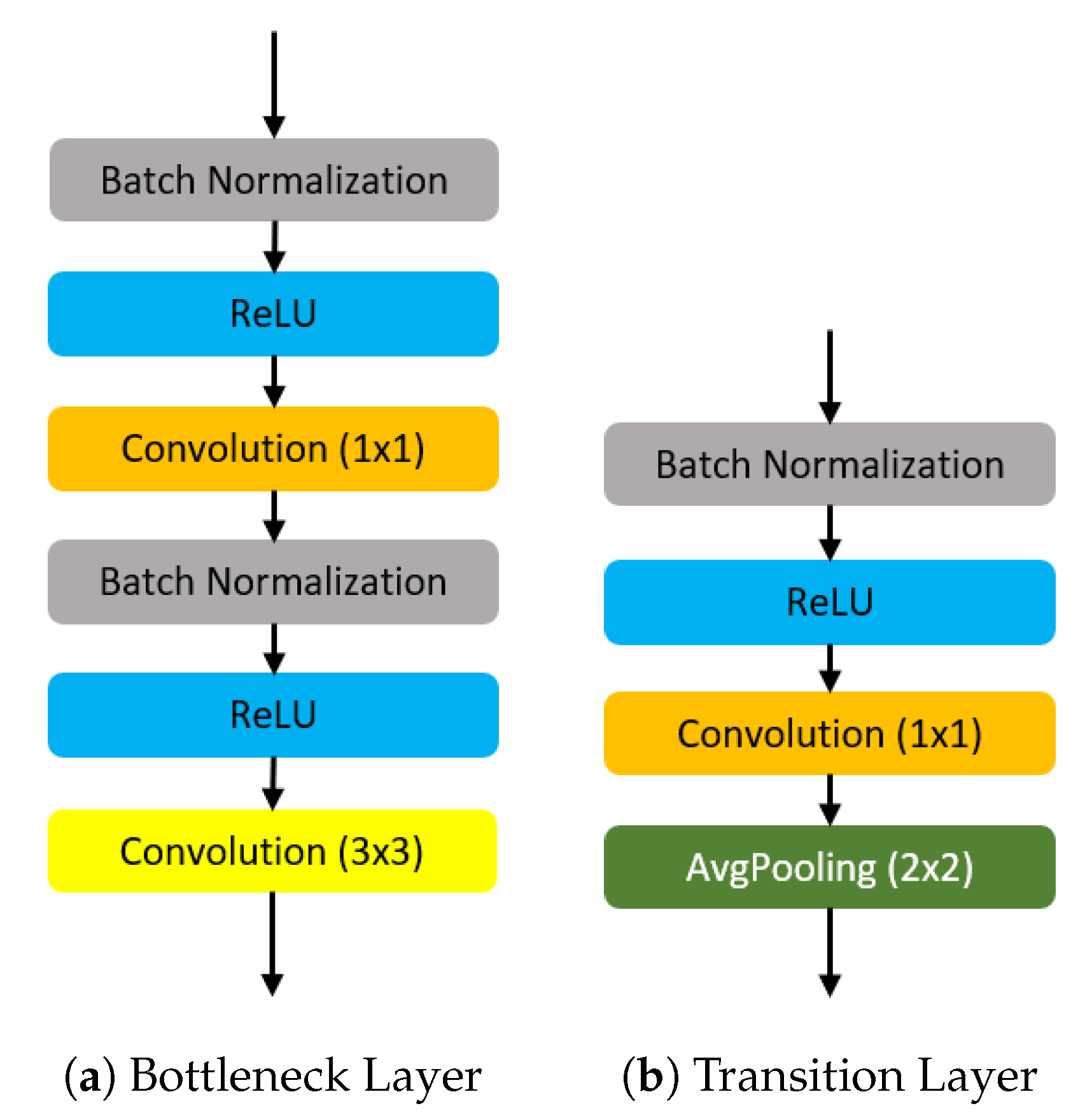
DenseNet is composed of dense block and transition layer. The dense block consists of a bottleneck layer and a growth rate. Since the feature maps of different layers in DenseNet are connected using channel-wise concatenation, but it can lead to oversized parameters of the network, which will affect the efficiency of the computation. To avoid oversized parameters’ problem, the DenseNet author used the growth rate (=k) as a hyperparameter, also apply the Batch Normalization (BN) -> Rectified Linear Unit (ReLU) -> Conv(1 × 1) -> Batch Normalization (BN) -> ReLU -> Conv(3 × 3) nonlinear transformation to the DenseNet structure in order to solve the problem we mentioned before. The bottleneck layer is shown in the Figure 6a. Additionally, as before, it is used to reduce the number of input feature maps and improve calculation efficiency.
As shown in Figure 6b, the transition layer has the role of reducing the width and height size of feature maps and reducing the number of feature maps. It is connected behind the dense block and consists of BN -> ReLU -> Conv(1 × 1) -> Avg pool(2 × 2). At this time, it is determined how much to reduce the feature map through the hyperparameter value between 0 and 1 called the compression factor. If this value is 1, the number of feature maps does not change. In addition, DenseNet applied the composite function consisting of the order of BN -> ReLU -> Conv to the layer, citing the efficiency results according to the order of BN, ReLU, and Conv tested in [28].
3.3.2. LSTM
LSTM is a special structure of RNN, a field of deep learning, and solves the long-term dependency problem. The long-term dependency problem says when past information is not delivered to the end. By solving these problems, LSTM shows good performance in analyzing and predicting not only short sentences but also long data such as voice and video and time-series data.
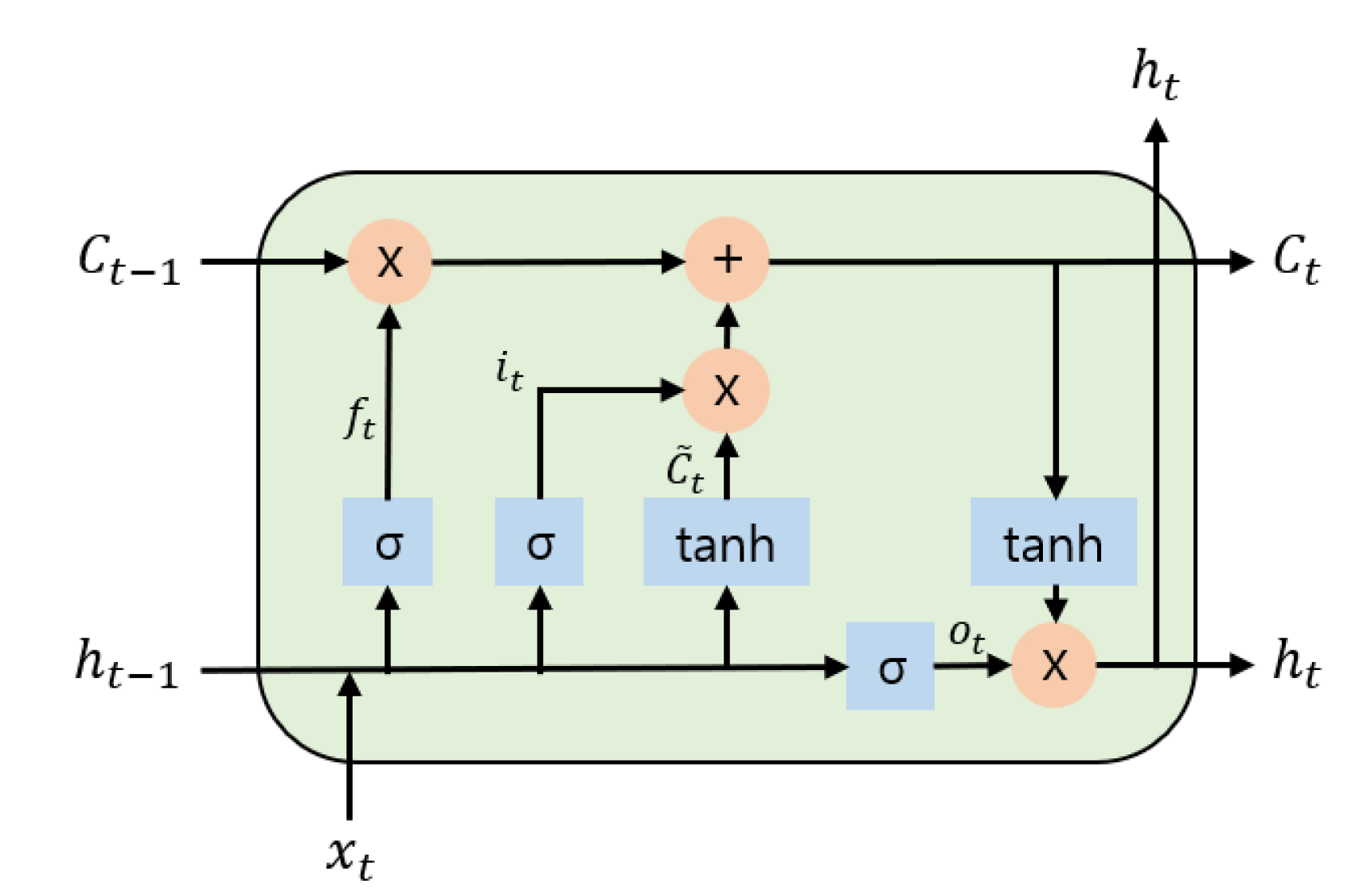
Figure 7 shows the structure of the LSTM. The top line in Figure 7 is the cell state, which is the core of the LSTM. The cell state flows like a conveyor belt, adding and subtracting information through the gate and sending the information to the next level. It’s also makes the previous information directly influence the future output. LSTM basically goes through four steps. The first step is the forget gate layer, expressed by Equation (1). In this step, it is used to decide what information to forget by the sigmoid layer. is the input vector to the LSTM unit, is the previous hidden state vector which can be seen as the output vector of the previous LSTM unit. , also means the weight matrices and bias vector parameters for forget alyer which need to be optimized during model training. is a sigmoid function, the sigmoid functions return values (y axis) in the range 0 to 1, and the LSTM unit will select which value in the range of 0 to 1 to forget. The second step is the input gate layer of Equation (2) and the tanh layer of Equation (3). The input gate layer determines which values to update through the sigmoid layer, and the tanh layer creates a new candidate value of which is a cell input activation vector. Finally, the values of the two layers are added and appended to the cell state. The third step is to create a new cell state by updating the past state as shown in Equation (4). First, the information decided to be dropped through the forget gate is discarded, and the information decided to be added is appended next. The last step is the part to decide which value to output with the output gate layer of Equation (5). First, determine which part of the cell state is to be exported through sigmoid for input data, and determine the final output by multiplying the value obtained through the tanh layer in the cell state as shown in Equation (6).
3.3.3. Hybrid Model
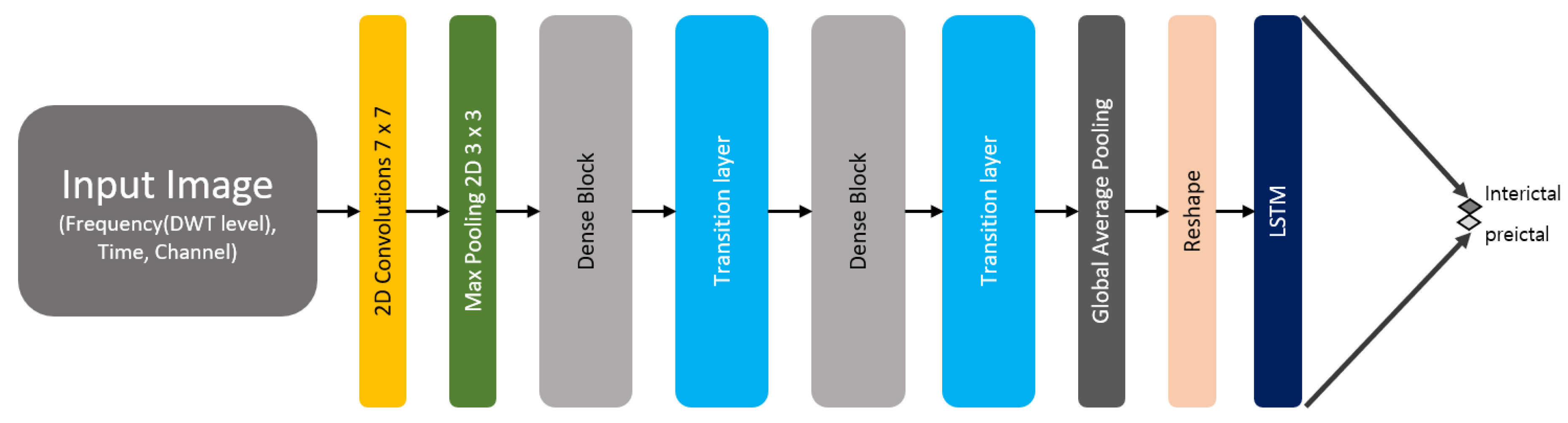
As shown in Figure 8, we propose a hybrid model that combines DenseNet and LSTM. The proposed model uses the structure of DenseNet to construct the first half. We use the feature map from here as input data of LSTM to reflect the sequence information on the feature and finally propose a hybrid model that classifies through the sigmoid function. Specifically, the input data are image data converted by applying DWT to the raw EEG signal and are composed of frequency (DWT level), time, and channel. The input image first passes through the Conv layer and makes an output feature map that is twice the growth rate. Next, all dense blocks each have the same number of layers, and Conv(3 × 3) in them does 1-pixel zero-padding so that the size of the feature map does not change. After the dense block, the transition layer is used. Transition layers reduce the size of the feature map through Conv(1 × 1) and apply average pooling. Finally, instead of a fully connected layer that increases parameters too much, global average pooling is used to create and output the feature map as a 1-D vector. Then, through reshape, it is converted into an input format suitable for LSTM and input into LSTM. Finally, the features generated through LSTM are classified into interictal and preictal states using the Sigmoid function. The detailed structure is shown in Table 1.
4. Performance Evaluation
4.1. Experimental Setup
This section describes the workstation environment, hyperparameters of DenseNet-LSTM, experimental methods, and evaluation indicators. As shown in Table 2, AMD Ryzen 7 3700X was used as the CPU, and a total of 64 GB of memory was used. The proposed model was trained using GeForce RTX 2080 Ti as GPU. The software is experimented with using Python 3.6 version, Tensorflow 1.14, and Keras 2.2.4 version. As a hyperparameter of DenseNet-LSTM, as shown in the Table 3, the growth rate was set to 32, and the compression factor was set to 0.5. For the activation function, ReLU was used, Adam was selected as the optimizer, and the learning rate was set to 0.001.
The experimental method is performed using the k-fold cross-validation method. K-fold cross-validation divides the data into k folds, trains with k − 1, and tests with the remaining one. The average of the result values obtained by repeating this process k times is used as the verification result of the model.
In order to evaluate the seizure prediction performance of the model, accuracy, sensitivity, specificity, and FPR (False prediction rate), F1-score calculated as shown in Table 4 are used as performance indicators. Accuracy represents the proportion of correctly classified data in the entire dataset. Sensitivity represents the ratio accurately predicted as preictal among data classified as preictal. Specificity refers to the ratio predicted by the actual interictal among data classified as interictal, and FPR refers to the ratio of incorrectly judging the interictal as preictal states. Precision is the ratio of really true among true predicted values. F1-score represents the harmonic average of precision and recall.
4.2. Experimental Results
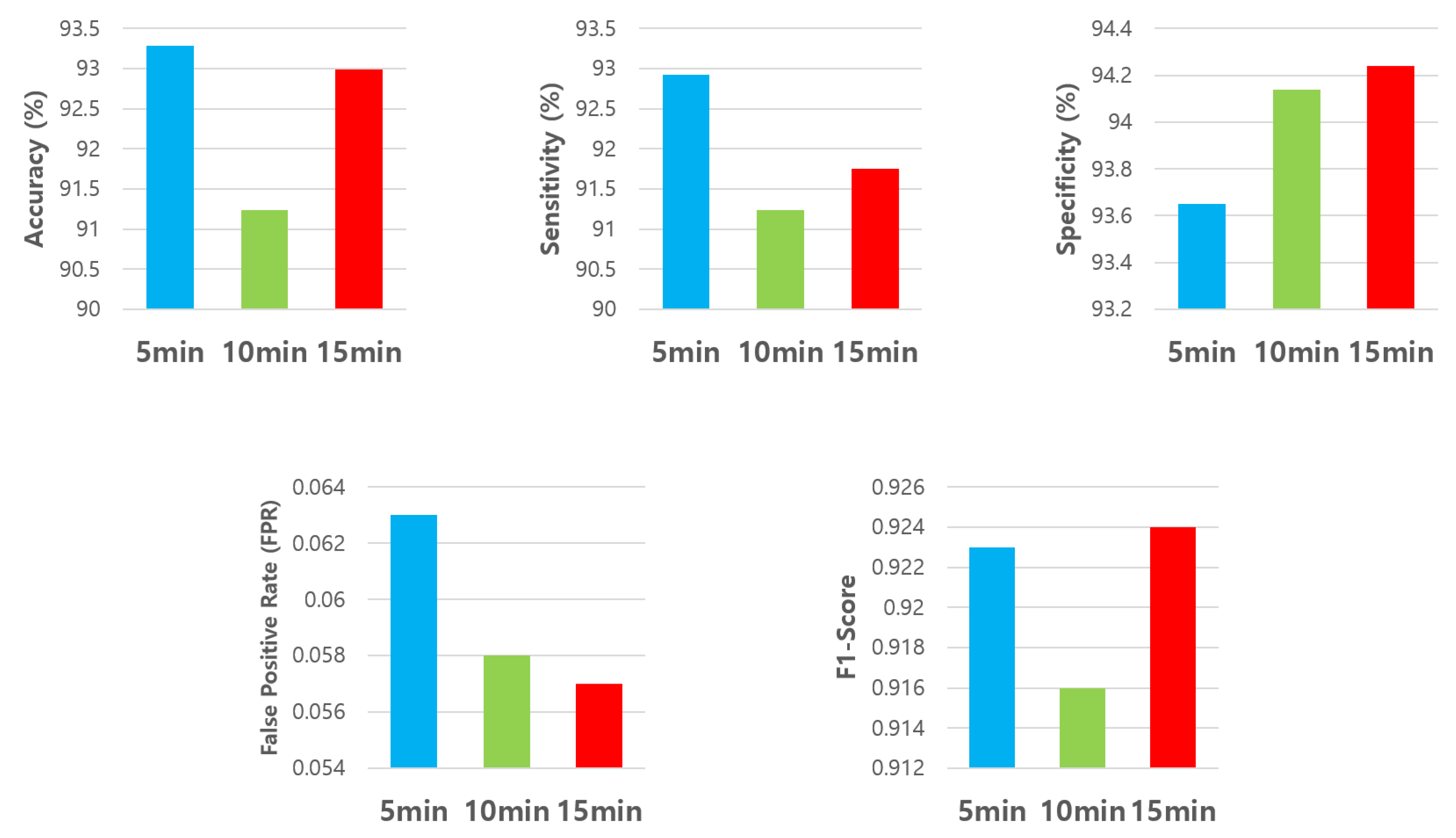
In this section, we set the preictal lengths to 5, 10, and 15 min, respectively, and show the experimental results and comparison with the existing algorithm. Figure 9 shows the average Acc, Sen, Spec, FPR, F1-score over 5, 10, and 15 min of preictal lengths. In the experimental results, the model trained under the assumption that the preictal length of 5 min ensures a higher sensitivity than that of 10 and 15 min. This means that the model assumed to be 5 min trained the preictal interval better than other models, so the preictal characteristic appears a lot between 0 and 5 min. On the other hand, assuming that the preictal lengths are 10 and 15 min, the trained model has a higher specificity and lower FPR than 5 min. This means that the model trained to assume 10 and 15 min clearly distinguished the interval classified as interictal than other models.
Table 5 shows the average Acc, Sen, Spec, FPR, and F1-score for each patient according to the preictal length. Looking at the results for each patient, the average sensitivity is high in the model assuming the preictal length of 5 min, but in the case of patient 4, the sensitivity is lower than 10 and 15 min and the specificity is high. It can be seen that the preictal characteristics did not appear well during 0–5 min and appeared after 5 min. On the other hand, in the case of patient 24, the sensitivity of the trained model was relatively lower than that of 5 min, assuming the preictal length was 10 and 15 min. This means that the preictal features were more pronounced at 0–5 min. In addition, the overall average result is best when the preictal length is assumed to be 5 min. However, the model that predicted the balanced outcome without significantly degrading the outcome for each patient was when the preictal length was 15 min.
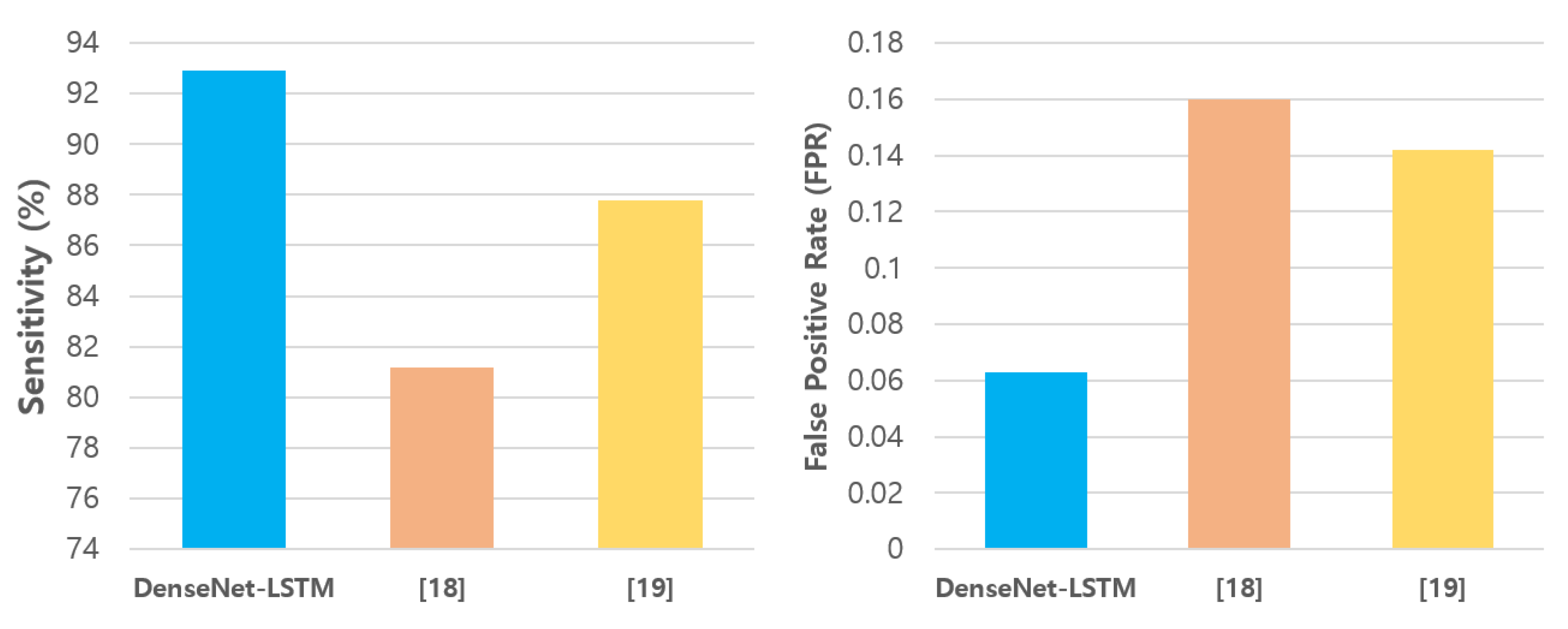
In order to objectively verify the performance of our proposed method, we compared it with the existing algorithms [22,23,24]. The authors of [22] proposed a method of converting EEG signals into image data through STFT and classifying them through CNN. In [23], an EEG signal is transformed into image data through CWT and uses CNN for classification. The authors of [24] predicted seizures using features obtained through Hjorth parameters as input to 3D-CNN. As shown in Figure 10 and Table 6, the proposed method has better performance than the existing method. This means that the proposed model is different from the CNN used in the existing algorithm, using the improved DenseNet method and reinforcing the information flow throughout the network, so that the learning was effective. In addition, it can be said that the sequence information of the EEG signal was well learned by adding the LSTM in the second half.
5. Conclusions
In this paper, we have proposed a new deep learning hybrid model, DenseNet-LSTM for predicting patient-specific epileptic seizures using scalp EEG data. This method achieves a prediction accuracy of 93.28%, a sensitivity of 92.92%, a specificity of 93.65%, an FPR of 0.063 per hour, and an F1-score of 0.923. The DenseNet approach, which improves the existing CNN problem proposed in this study, enhances the information flow throughout the network and increases computational efficiency. In addition, by applying LSTM, the long-term temporal features of the EEG data are trained by the network. Since the CHB-MIT dataset used in the proposed method consists mostly of pediatric patients, it needs to be extensively tested with more EEG data. However, our experimental results and comparisons with previous studies show that the proposed method is efficient and reliable. This suggests the potential as a seizure prediction tool to effectively mitigate the potential threat of epilepsy patients.
Author Contributions
Conceptualization, S.R. and I.J.; methodology, S.R.; software, S.R.; validation, S.R. and I.J.; investigation, S.R.; resources, S.R.; data curation, S.R.; writing—original draft preparation, S.R.; writing—review and editing, I.J.; visualization, S.R.; supervision, I.J.; project administration, I.J.; funding acquisition, I.J. All authors have read and agreed to the published version of the manuscript.
Funding
This work was supported by Institute for Information & communications Technology Promotion (IITP) grant funded by the Korea government (MSIP) (No. 2020-0-00107, Development of the technology to automate the recommendations for big data analytic models that define data characteristics and problems).
Institutional Review Board Statement
Not applicable.
Informed Consent Statement
Not applicable.
Data Availability Statement
The CHB-MIT Scalp EEG Database is available at https://physionet.org/content/chbmit/1.0.0/ (accessed on 9 June 2020).
Conflicts of Interest
The authors declare no conflict of interest.
References
- Fisher, R.S.; Acevedo, C.; Arzimanoglou, A.; Bogacz, A.; Cross, J.H.; Elger, C.E.; Engel, J., Jr.; Forsgren, L.; French, J.A.; Glynn, M.; et al. ILAE official report: A practical clinical definition of epilepsy. Epilepsia 2014, 55, 475–482. [Google Scholar] [CrossRef] [Green Version]
- World Health Organization. Neurological Disorders: Public Health Challenges; World Health Organization: Geneva, Switzerland, 2006. [Google Scholar]
- Chiang, C.Y.; Chang, N.F.; Chen, T.C.; Chen, H.H.; Chen, L.G. Seizure prediction based on classification of EEG synchronization patterns with on-line retraining and post-processing scheme. In Proceedings of the 2011 Annual International Conference of the IEEE Engineering in Medicine and Biology Society, Boston, MA, USA, 30 August–3 September 2011; pp. 7564–7569. [Google Scholar]
- Krizhevsky, A.; Sutskever, I.; Hinton, G.E. Imagenet classification with deep convolutional neural networks. Commun. ACM 2017, 60, 84–90. [Google Scholar] [CrossRef]
- Huang, G.; Liu, Z.; Van Der Maaten, L.; Weinberger, K.Q. Densely connected convolutional networks. In Proceedings of the 2017 IEEE Conference on Computer Vision and Pattern Recognition (CVPR), Honolulu, HI, USA, 21–26 July 2017; pp. 4700–4708. [Google Scholar]
- Hochreiter, S.; Schmidhuber, J. Long short-term memory. Neural Comput. 1997, 9, 1735–1780. [Google Scholar] [CrossRef] [PubMed]
- Maiwald, T.; Winterhalder, M.; Aschenbrenner-Scheibe, R.; Voss, H.U.; Schulze-Bonhage, A.; Timmer, J. Comparison of three nonlinear seizure prediction methods by means of the seizure prediction characteristic. Phys. D Nonlinear Phenom. 2004, 194, 357–368. [Google Scholar] [CrossRef]
- Winterhalder, M.; Schelter, B.; Maiwald, T.; Brandt, A.; Schad, A.; Schulze-Bonhage, A.; Timmer, J. Spatio-temporal patient–individual assessment of synchronization changes for epileptic seizure prediction. Clin. Neurophysiol. 2006, 117, 2399–2413. [Google Scholar] [CrossRef] [PubMed]
- Li, S.; Zhou, W.; Yuan, Q.; Liu, Y. Seizure prediction using spike rate of intracranial EEG. IEEE Trans. Neural Syst. Rehabil. Eng. 2013, 21, 880–886. [Google Scholar] [CrossRef] [PubMed]
- Zheng, Y.; Wang, G.; Li, K.; Bao, G.; Wang, J. Epileptic seizure prediction using phase synchronization based on bivariate empirical mode decomposition. Clin. Neurophysiol. 2014, 125, 1104–1111. [Google Scholar] [CrossRef] [PubMed]
- Eftekhar, A.; Juffali, W.; El-Imad, J.; Constandinou, T.G.; Toumazou, C. Ngram-derived pattern recognition for the detection and prediction of epileptic seizures. PLoS ONE 2014, 9, e96235. [Google Scholar] [CrossRef] [PubMed]
- Elgohary, S.; Eldawlatly, S.; Khalil, M.I. Epileptic seizure prediction using zero-crossings analysis of EEG wavelet detail coefficients. In Proceedings of the 2016 IEEE Conference on Computational Intelligence in Bioinformatics and Computational Biology (CIBCB), Chiang Mai, Thailand, 5–7 October 2016; pp. 1–6. [Google Scholar]
- Tsiouris, K.M.; Pezoulas, V.C.; Koutsouris, D.D.; Zervakis, M.; Fotiadis, D.I. Discrimination of preictal and interictal brain states from long-term EEG data. In Proceedings of the 2017 IEEE 30th International Symposium on Computer-Based Medical Systems (CBMS), Thessaloniki, Greece, 22–24 June 2017; pp. 318–323. [Google Scholar]
- Sharif, B.; Jafari, A.H. Prediction of epileptic seizures from EEG using analysis of ictal rules on Poincaré plane. Comput. Methods Programs Biomed. 2017, 145, 11–22. [Google Scholar] [CrossRef] [PubMed]
- Akut, R. Wavelet based deep learning approach for epilepsy detection. Health Inf. Sci. Syst. 2019, 7, 8. [Google Scholar] [CrossRef] [PubMed]
- Boonyakitanont, P.; Lek-uthai, A.; Chomtho, K.; Songsiri, J. A Comparison of Deep Neural Networks for Seizure Detection in EEG Signals. bioRxiv 2019, 702654. [Google Scholar] [CrossRef]
- Karim, A.M.; Karal, Ö.; Çelebi, F. A new automatic epilepsy serious detection method by using deep learning based on discrete wavelet transform. In Proceedings of the 3rd International Conference on Engineering Technology and Applied Sciences (ICETAS), Skopje, North Macedonia, 17–21 July 2018; Volume 4, pp. 15–18. [Google Scholar]
- Liang, W.; Pei, H.; Cai, Q.; Wang, Y. Scalp EEG epileptogenic zone recognition and localization based on long-term recurrent convolutional network. Neurocomputing 2020, 396, 569–576. [Google Scholar] [CrossRef]
- Park, Y.; Luo, L.; Parhi, K.K.; Netoff, T. Seizure prediction with spectral power of EEG using cost-sensitive support vector machines. Epilepsia 2011, 52, 1761–1770. [Google Scholar] [CrossRef] [PubMed]
- Zhang, Z.; Parhi, K.K. Low-complexity seizure prediction from iEEG/sEEG using spectral power and ratios of spectral power. IEEE Trans. Biomed. Circuits Syst. 2015, 10, 693–706. [Google Scholar] [CrossRef] [PubMed]
- Cho, D.; Min, B.; Kim, J.; Lee, B. EEG-based prediction of epileptic seizures using phase synchronization elicited from noise-assisted multivariate empirical mode decomposition. IEEE Trans. Neural Syst. Rehabil. Eng. 2016, 25, 1309–1318. [Google Scholar] [CrossRef] [PubMed]
- Truong, N.D.; Nguyen, A.D.; Kuhlmann, L.; Bonyadi, M.R.; Yang, J.; Ippolito, S.; Kavehei, O. Convolutional neural networks for seizure prediction using intracranial and scalp electroencephalogram. Neural Netw. 2018, 105, 104–111. [Google Scholar] [CrossRef] [PubMed] [Green Version]
- Khan, H.; Marcuse, L.; Fields, M.; Swann, K.; Yener, B. Focal onset seizure prediction using convolutional networks. IEEE Trans. Biomed. Eng. 2017, 65, 2109–2118. [Google Scholar] [CrossRef] [Green Version]
- Ozcan, A.R.; Erturk, S. Seizure prediction in scalp EEG using 3D convolutional neural networks with an image-based approach. IEEE Trans. Neural Syst. Rehabil. Eng. 2019, 27, 2284–2293. [Google Scholar] [CrossRef]
- Shoeb, A.H. Application of Machine Learning to Epileptic Seizure Onset Detection and Treatment. Ph.D. Thesis, Massachusetts Institute of Technology, Cambridge, MA, USA, 2009. [Google Scholar]
- Choi, G.; Park, C.; Kim, J.; Cho, K.; Kim, T.J.; Bae, H.; Min, K.; Jung, K.Y.; Chong, J. A Novel Multi-scale 3D CNN with Deep Neural Network for Epileptic Seizure Detection. In Proceedings of the 2019 IEEE International Conference on Consumer Electronics (ICCE), Las Vegas, NV, USA, 11–13 January 2019; pp. 1–2. [Google Scholar]
- Heil, C.E.; Walnut, D.F. Continuous and discrete wavelet transforms. SIAM Rev. 1989, 31, 628–666. [Google Scholar] [CrossRef] [Green Version]
- He, K.; Zhang, X.; Ren, S.; Sun, J. Identity mappings in deep residual networks. In Proceedings of the European Conference on Computer Vision, Amsterdam, The Netherlands, 8–16 October 2016; pp. 630–645. [Google Scholar]
Figure 1.
An example of epileptic brain states which contains an interictal part, preictal part, ictal part and postictal part.The horizontal axis displays the time and the vertical axis displays the measured voltage.
Figure 1.
An example of epileptic brain states which contains an interictal part, preictal part, ictal part and postictal part.The horizontal axis displays the time and the vertical axis displays the measured voltage.

Figure 2.
The system model of proposed method.

Figure 3.
Preictal length.

Figure 4.
The process of converting raw EEG signals into time-frequency images using DWT.

Figure 5.
An example of dense connectivity. The square means the input feature maps with several channels. The curve connects the previous feature map with next layer feature map using channel-wise concatenation.
Figure 5.
An example of dense connectivity. The square means the input feature maps with several channels. The curve connects the previous feature map with next layer feature map using channel-wise concatenation.

Figure 6.
Bottleneck layer and transition layer. Batch normalization is performed independently for each feature map, the ReLU is a piecewise linear function that will output directly if the input is positive; otherwise, it will output zero. As for the 1 × 1 convolution is used to reduce the number of feature maps to improve the computational efficiency.

Figure 7.
Structure of the LSTM cell.

Figure 8.
Architecture of DenseNet-LSTM.

Figure 9.
Average of accuracy, sensitivity, specificity, false positive rate and F1-score according to preictal lengths of 5, 10, 15 min.
Figure 9.
Average of accuracy, sensitivity, specificity, false positive rate and F1-score according to preictal lengths of 5, 10, 15 min.


Table 1.
Structure of DenseNet-LSTM.
| Layers | Feature Map Size | Configuration |
|---|---|---|
| Convolution Layer | 3 × 1280 × 64 | , stride 2 |
| Dense Block 1 | 2 × 640 × 256 | |
| Transition Layer 1 | 2 × 640 × 128 | |
| 1 × 320 × 128 | 2 × 2 average pooling, stride2 | |
| Dense Block 2 | 1 × 320 × 512 | |
| Transition Layer 2 | 1 × 320 × 256 | |
| 1 × 160 × 256 | 2 × 2 average pooling, stride2 | |
| LSTM Layer | 1 × 256 | global average pooling |
| 4 × 64 | reshape | |
| 1 × 128 | LSTM layer | |
| Classification Layer | 1 × 1 | sigmoid |
Table 2.
Workstation configuration.
| Software or Hardware | Specification |
|---|---|
| CPU | AMD Ryzen 7 3700X |
| GPU | GeForce RTX 2080 Ti |
| RAM | DDR4 64 GB |
| Python | 3.6 |
| Tensorflow | 1.14 |
| Keras | 2.2.4 |
Table 3.
Hyperparameter configuration.
| Hyperparameters | Values |
|---|---|
| Growth rate | 32 |
| Compression factor | 0.5 |
| Activation function | ReLU |
| Optimizer | Adam |
| Learning rate | 0.001 |
Table 4.
Evaluation metrics (TP is true positive, TN is true negative, FP is false positive, FN is false negative).
Table 4.
Evaluation metrics (TP is true positive, TN is true negative, FP is false positive, FN is false negative).
| Performance Indicator | Formula |
|---|---|
| Accuracy | (TP + TN)/(TP + TN + FP + FN) |
| Sensitivity (Recall) | TP/(TP + FN) |
| Specificity | TN/(TN + FP) |
| Precision | TP/(TP + FP) |
| False Positive Rate (FPR) | FP/(TN + FP) |
| F1-Score | 2 × ((Precision × Recall)/(Precision + Recall)) |
Table 5.
Seizure prediction results according to preictal length in 24 patients from the CHB-MIT scalp EEG dataset.
Table 5.
Seizure prediction results according to preictal length in 24 patients from the CHB-MIT scalp EEG dataset.
| Patient | Preictal Length: 5 min | Preictal Length: 10 min | Preictal Length: 15 min | ||||||||||||
|---|---|---|---|---|---|---|---|---|---|---|---|---|---|---|---|
| Accuracy | Sensitivity | Specificity | FPR | F1-Score | Accuracy | Sensitivity | Specificity | FPR | F1-Score | Accuracy | Sensitivity | Specificity | FPR | F1-Score | |
| chb01 | 100% | 100% | 100% | 0 | 1 | 100% | 100% | 100% | 0 | 1 | 99.97% | 99.95% | 100% | 0 | 0.999 |
| chb02 | 86.94% | 87.97% | 85.91% | 0.141 | 0.869 | 89.89% | 80.79% | 98.98% | 0.01 | 0.877 | 91.47% | 82.94% | 100% | 0 | 0.897 |
| chb03 | 96.82% | 96.3% | 97.33% | 0.026 | 0.967 | 86.86% | 74.49% | 99.23% | 0.007 | 0.808 | 93.66% | 88.77% | 98.54% | 0.014 | 0.929 |
| chb04 | 78.26% | 65.46% | 91.06% | 0.089 | 0.687 | 90.46% | 89.8% | 91.11% | 0.089 | 0.9 | 90.78% | 83.61% | 97.95% | 0.02 | 0.894 |
| chb05 | 94.32% | 97.82% | 90.83% | 0.091 | 0.946 | 97.29% | 96.56% | 98.02% | 0.02 | 0.972 | 98.76% | 98.54% | 98.99% | 0.01 | 0.987 |
| chb06 | 94.2% | 88.61% | 99.78% | 0.002 | 0.902 | 96.6% | 95.41% | 97.79% | 0.022 | 0.963 | 87.34% | 86.9% | 87.78% | 0.122 | 0.861 |
| chb07 | 100% | 100% | 100% | 0 | 1 | 99.4% | 98.81% | 100% | 0 | 0.993 | 100% | 100% | 100% | 0 | 1 |
| chb08 | 100% | 100% | 100% | 0 | 1 | 100% | 100% | 100% | 0 | 1 | 100% | 100% | 100% | 0 | 1 |
| chb09 | 99.82% | 99.65% | 100% | 0 | 0.998 | 99.64% | 99.28% | 100% | 0 | 0.996 | 99.9% | 99.97% | 99.83% | 0.001 | 0.999 |
| chb10 | 90.52% | 94.11% | 86.94% | 0.13 | 0.916 | 91.58% | 90.45% | 92.72% | 0.072 | 0.913 | 90.78% | 89.48% | 92.09% | 0.079 | 0.904 |
| chb11 | 100% | 100% | 100% | 0 | 1 | 100% | 100% | 100% | 0 | 1 | 99.58% | 99.21% | 99.94% | 0 | 0.995 |
| chb12 | 93.07% | 86.99% | 99.16% | 0.008 | 0.879 | 95.91% | 94.39% | 97.43% | 0.025 | 0.953 | 96.46% | 95.06% | 97.86% | 0.021 | 0.961 |
| chb13 | 92.05% | 94.41% | 89.69% | 0.103 | 0.922 | 91.05% | 88.19% | 93.9% | 0.06 | 0.901 | 89.62% | 86.61% | 92.62% | 0.073 | 0.889 |
| chb14 | 89.66% | 93.27% | 86.06% | 0.139 | 0.901 | 85.79% | 80.66% | 90.93% | 0.09 | 0.831 | 83.52% | 81.16% | 85.87% | 0.141 | 0.824 |
| chb15 | 89.41% | 95.46% | 83.36% | 0.166 | 0.902 | 74.97% | 77.12% | 72.82% | 0.272 | 0.74 | 80.54% | 81.97% | 79.12% | 0.208 | 0.817 |
| chb16 | 81.03% | 71.2% | 90.86% | 0.091 | 0.778 | 81.33% | 71.4% | 91.27% | 0.087 | 0.77 | 87.16% | 86.53% | 87.79% | 0.122 | 0.872 |
| chb17 | 100% | 100% | 100% | 0 | 1 | 99.8% | 100% | 99.6% | 0.004 | 0.998 | 100% | 100% | 100% | 0 | 1 |
| chb18 | 92.35% | 91.06% | 93.64% | 0.063 | 0.92 | 93.23% | 95.72% | 90.73% | 0.092 | 0.936 | 86.39% | 92.53% | 80.24% | 0.197 | 0.877 |
| chb19 | 100% | 100% | 100% | 0 | 1 | 100% | 100% | 100% | 0 | 1 | 100% | 100% | 100% | 0 | 1 |
| chb20 | 99.96% | 100% | 99.93% | 0 | 0.999 | 99.86% | 100% | 99.72% | 0.002 | 0.998 | 99.88% | 100% | 99.77% | 0.002 | 0.998 |
| chb21 | 95.4% | 93.81% | 96.99% | 0.03 | 0.952 | 93.36% | 91.87% | 94.83% | 0.051 | 0.932 | 90.81% | 88.8% | 92.81% | 0.071 | 0.906 |
| chb22 | 81.61% | 93.24% | 69.98% | 0.3 | 0.836 | 81.61% | 88.43% | 74.79% | 0.252 | 0.828 | 87.78% | 87.87% | 87.69% | 0.123 | 0.876 |
| chb23 | 96.66% | 96.01% | 97.32% | 0.026 | 0.966 | 91.01% | 99.05% | 82.97% | 0.17 | 0.933 | 93.86% | 99.61% | 88.1% | 0.119 | 0.95 |
| chb24 | 86.86% | 84.76% | 88.96% | 0.11 | 0.825 | 84.93% | 77.47% | 92.38% | 0.076 | 0.755 | 83.7% | 72.57% | 94.83% | 0.051 | 0.758 |
| Average | 93.28% | 92.92% | 93.65% | 0.063 | 0.923 | 92.69% | 91.24% | 94.13% | 0.058 | 0.916 | 92.99% | 91.75% | 94.24% | 0.057 | 0.924 |
Table 6.
Results of a recent epileptic seizure prediction approach on the CHB-MIT scalp EEG dataset. In the case of “This work”, the results of 5 min of preictal length, which had the best results, were used.
Table 6.
Results of a recent epileptic seizure prediction approach on the CHB-MIT scalp EEG dataset. In the case of “This work”, the results of 5 min of preictal length, which had the best results, were used.
| Authors | Year | Datasts | Features | Classifier | Acc (%) | Sen (%) | Spec (%) | FPR (H) | F1-Score |
|---|---|---|---|---|---|---|---|---|---|
| Khan et al. [23] | 2017 | CHB-MIT, 15 patients | Continuous wavelet transform | CNN | - | 87.8 | - | 0.147 | - |
| Truong et al. [22] | 2018 | CHB-MIT, 13 patients | Short-time Fourier transform | CNN | - | 81.2 | - | 0.16 | - |
| Ozcan et al. [24] | 2019 | CHB-MIT, 16 patients | Hjorth parameters | 3D CNN | - | 85.71 | - | 0.096 | - |
| This work | 2021 | CHB-MIT, 24 patients | Discrete wavelet transform | DenseNet-LSTM | 93.28 | 92.92 | 93.65 | 0.063 | 0.923 |
Publisher’s Note: MDPI stays neutral with regard to jurisdictional claims in published maps and institutional affiliations. |
© 2021 by the authors. Licensee MDPI, Basel, Switzerland. This article is an open access article distributed under the terms and conditions of the Creative Commons Attribution (CC BY) license (https://creativecommons.org/licenses/by/4.0/).
Share and Cite
MDPI and ACS Style
Ryu, S.; Joe, I. A Hybrid DenseNet-LSTM Model for Epileptic Seizure Prediction. Appl. Sci. 2021, 11, 7661. https://doi.org/10.3390/app11167661
AMA Style
Ryu S, Joe I. A Hybrid DenseNet-LSTM Model for Epileptic Seizure Prediction. Applied Sciences. 2021; 11(16):7661. https://doi.org/10.3390/app11167661
Chicago/Turabian StyleRyu, Sanguk, and Inwhee Joe. 2021. "A Hybrid DenseNet-LSTM Model for Epileptic Seizure Prediction" Applied Sciences 11, no. 16: 7661. https://doi.org/10.3390/app11167661
Note that from the first issue of 2016, this journal uses article numbers instead of page numbers. See further details here.