Can a Weather-Based Crop Insurance Scheme Increase the Technical Efficiency of Smallholders? A Case Study of Groundnut Farmers in India

Abstract

This paper analyzes the impact of a Weather-Based Crop Insurance Scheme (WBCIS) on the Technical Efficiency (TE) of smallholder groundnut farmers in the context of climate change in India. We use Data Envelopment Analysis (DEA) to study the TE of smallholder farmers, which range between 0.58 and 1, with a mean of 0.79. Using the Propensity Score Matching (PSM) technique, we find that the TE of smallholder farmers improves when they participate in a WBCIS using three matching methods. Increasing the coverage of farmers under a WBCIS can help in reducing smallholder farmers vulnerability to climate change.

1. Introduction

Studying the impact of climate change on smallholder agriculture and devising appropriate policy and program measures are at the top of the policy agenda in developing countries. Yet, it is not clear which types of interventions can reduce the vulnerability of smallholder farmers, improve their production efficiency, and build long-term resiliency of the farming systems. In this paper, we analyze the impact of participating in a Weather-Based Crop Insurance Scheme (WBCIS) on the Technical Efficiency (TE) of smallholder groundnut farmers in India. In the rest of this section, we introduce the importance of a WBCIS in reducing the climate change vulnerability of smallholder farmers in India. Section two presents the objectives of the study. Section three presents the materials and methods. Results and discussions are presented in section four. Summary and conclusions form the last section.

The Ananthapuramu district in Andhra Pradesh, India, was purposively selected for this in-depth study, as the district is drought-prone, with 90 percent of its cultivated area being under rain-fed conditions, and it ranks second among the lowest rainfall districts in India (after Jaisalmer in the State of Rajasthan, with 165 mm rainfall). It is well known that low and erratic rainfall patterns can have detrimental impact on crop production. As groundnut is the major crop cultivated in the study district (around 51% of gross area sown [1], understanding the influence of rainfall variability on groundnut production is important for designing appropriate interventions to reduce the vulnerability of smallholders and to increase their resilience. Filling such an evidence gap is also useful to smallholder farmers to allow them to adopt strategies that lessen the impact of climate risks on crop production. In this context, climate adaptation is considered an essential strategy for responding to climate change in a locality to sustain agricultural production. Interventions such as the adoption of water saving crop production technologies, cultivation of drought resistant and high yielding crop varieties, drought proofing measures, micro-credit services, and participation in a WBCIS implemented by the Government of Andhra Pradesh in 2007 [2] are considered as important measures to ensure sustainable crop production in the context of climatic risks. Among these interventions, participation of smallholder farmers in a WBCIS is seen as the best possible climate adaptation strategy, as it reduces the hardship of insured farmers against financial loss arising out of adverse weather conditions. This scheme is a unique weather-based insurance product designed to provide protection to the farmer–beneficiaries against a decline in crop yields resulting from adverse rainfall incidences (both deficit and excess) during the Kharif season and adverse incidences in other weather parameters such as relative humidity and unseasonal rainfall during the Rabi season. With the increase in production risks in the study district during both the Kharif and Rabi seasons, the Government has been implementing several safety nets to the farming community, namely, debt-waiver schemes, paying compensations through the National Disaster-Relief Fund, price support programs, production subsidies, and production loans at concessional rates of interest, so as to sustain them in agri-business. However, the provision of these safety nets to needy farmers suffers from lack of a scientific approach, both in terms of quantifying the risk and transparency in paying the compensation. It is in this context that the Government of Andhra Pradesh has been implementing a WBCIS in Ananthapuramu on a large-scale since 2007, and with the advent of climate change, it is gaining wider acceptance among the farming community. This scheme further offers insurance coverage at the lowest possible cost, and the beneficiaries receive secured incomes through climate risk management. In the earlier studies, the impact of weather insurance on production risk and farm income is well documented [3,4,5,6,7,8]. However, there is no previous study that investigated the impact of WBCIS on smallholder farmers’ TE in India. This is important because, improving farm TE is an important element to ensure cost-effective production. Therefore, the main objective of this paper is to evaluate the impact of the WBCIS on smallholder farmers’ TE in cultivating groundnut through employing Data Envelopment Analysis (DEA) and Propensity Scores Matching (PSM) methods. This study also suggests policy measures to promote the scheme, so as to reduce the farmers’ vulnerability in the context of climate change.

2. Objectives of the Study

This study has the following specific objectives:

• to study the trends in monthly, seasonal, and annual rainfall;
• to estimate the TE in groundnut production among the selected smallholder farmers;
• to analyze the impact of WBCIS on TE of groundnut production among smallholder farmers.

3. Materials and Methods

India ranks second in groundnut production in the world, after China. China is the leading producer (as well as consumer) of groundnut in the world with 17.15 m. tonnes of production during the period 2017–2018, followed by India (9.18 m. tonnes), the United States (3.28 m. tonnes), Nigeria (2.42 m. tonnes), and Sudan (1.64 m. tonnes). India leads other groundnut exporting countries such as Argentina, the USA, China, and Brazil. India is the largest exporter of groundnut in the world, with a share of about 28 percent in world trade during the period 2016–2017 [9]. Among the States in India, Gujarat leads in terms of groundnut area, with 1.59 m. ha, followed by Andhra Pradesh (0.76 m. ha), Rajasthan (0.67 m. ha), Karnataka (0.59 m. ha), Tamil Nadu (0.34 m. ha), and Madhya Pradesh (0.22 m. ha) during the period 2018–2019 [9]. Groundnut is mostly cultivated under rain-fed conditions in Andhra Pradesh, which increases it vulnerability to climatic variations. Ananthapuramu (0.49 m. ha), as well as Chittoor (0.11 m. ha) and Kurnool (0.10 m. ha), were key groundnut growing districts of Andhra Pradesh in the period 2018–2019. The high altitudes of the Western Ghats mountain range reduce the rainfall from the South-West monsoon. The rainfall during the North-East monsoon season is erratic, as it is influenced by depressions in the Bay of Bengal. So, the district receives a meagre rainfall of 542 mm (mean of the period 1926–2019 [1], and the erratic pattern of rainfall results in frequent droughts (Appendix A). Since the 1990s, with the advent of climate change, the variability of the rains has increased [10]. Further, with 82 percent of cultivable land is under red soils, the soil conditions do not help in water retention. [11]. These factors contribute to the increased vulnerability of groundnut farmers in the study area (Appendix B and Appendix C).

In Andhra Pradesh, Ananthapuramu ranks first in the cultivation of groundnut, with an area of 0.49 m. ha and production of 0.18 m. tonnes during the period 2018–2019. Within the district, the top two blocks (subdistricts) with the highest acreage of groundnut during the Kharif season 2018–2019, namely, Ramagiri of the Dharmavaram division (805 ha) and Talupula of the Kadiri division (784 ha), were purposively selected for this study [11]. From these two blocks, 161 smallholder groundnut farmers participating in the WBCIS (treated) and 315 smallholder groundnut farmers not participating in the WBCIS (untreated) were selected randomly for analysis. The relevant data for the study pertaining to the Kharif season during the year 2020 were obtained from the sampled farmers using a pre-tested questionnaire. The data pertaining to month-wise, season-wise, and annual rainfall during the period 1926–2019 and during the climate change period 1990–2019 was analyzed through computing mean, Standard Deviation (SD), and Coefficient of Variation (CV). Further, the following techniques were employed in the study to arrive at meaningful conclusions.

3.1. Data Envelopment Analysis (DEA)

This linear programming tool was employed to measure the TE of groundnut production in Ananthapuramu, considering an input-oriented DEA model [12,13] with Constant Returns to Scale (CRS). The main objective is to ascertain by how much input use must be reduced by an inefficient farm, given the level of output, in order for it to become efficient. Overall TE was measured and was distinguished into Pure TE and Scale efficiency. In this model, there are 476 (N) farms or Decision Making Units (DMUs), and each DMU uses four inputs (K) and produces one output (M). For the ith DMU, these are represented by the vectors x_i and y_i, respectively. Input variables include fertilizers, NPK (kg/ha), seed rate (kg/ha), gypsum (kg/ha), and organic manure (t/ha), and the output variable is groundnut output (kg). The selected inputs and the output are represented by a K × N input matrix, denoted by X, and an M × N output matrix, denoted by Y, respectively. For the ith DMU, the efficiency score of θ is obtained by solving the linear programming as follows:

min_θλθ

subject to:

−y_i + Y λ ≥ 0

θx_i − Xλ ≥ 0

λ ≥ 0

Here, θ indicates the input-oriented CRS efficiency score of the DMU under evaluation. If θ receive the value of 1 for a DMU, it indicates that the DMU is functioning with 100 percent efficiency and requires no current level of input reduction. On the contrary, if θ is less than 1, then that DMU is considered relatively less efficient and it could produce the same level of output while reducing the current input level. The values of θ range between 0 and 1 across the DMUs [14]. So, the value ‘1′ reflects that a unit cannot perform at more than 100 percent efficiency in the peer group. ‘λ’ is a vector of constants, describing the contribution of benchmark DMUs to the virtual DMU. Note that the linear programming problem must be solved N times, once for each DMU in the sample.

3.2. Propensity Score Matching (PSM)

The PSM technique was employed to analyze the impact of the WBCIS on the TE of groundnut production by smallholder farmers in the study area. The farmers who participate in the WBCIS are considered as treated (n = 161), and the farmers who did not participate in the WBCIS are considered as untreated (n = 315) categories. In this technique, each farmer in the treated category is matched with a farmer in the untreated category based on the observable covariates viz., age of the farmers (AGE), Land Holding Size (LHS), education (EDU), Good Agricultural Practices (GAPs), Farming Experience (FE), and Timeliness of farm operations (TIME). This will facilitate the assignment of treatments randomly across the two categories to analyze the average differences in TE. The PSM can be expressed as:

p(X) = Pr [D = 1|X] = E[D|X]; p(X) = F{h(X_i)},

(1)

where p(X) is a propensity score and Pr is the probability of adopting WBCIS (treated farmer will receive the value of ‘1′, and ‘0′ otherwise), conditional on the vector of covariates mentioned earlier.

The Probit model was employed to estimate the predicted probabilities (propensity scores) of adopting WBCIS [15,16,17]. The computed probabilities are used for matching the treated and untreated categories of farmers by employing three matching algorithms [18], namely, Nearest Neighbour Matching (NNM), Kernel-Based Matching (KBM), and Radius Matching (RM). From these three matching methods, Average Treatment Effect on the Treated (ATT), Average Treatment Effect (ATE), and Average Treatment on Untreated (ATU) are computed. Further, the Rosenbaum bound test was used to analyze the sensitivity of the estimated ATT to unobserved confounders [19,20].

4. Results and Discussion

4.1. Rainfall Variability in the Context of Climate Change

Monthly rainfall data were collected from the Agricultural Research Station (ARS) in Ananthapuramu, maintained by the Acharya NG Ranga Agricultural University (ANGRAU). Mean, SD, and CV were computed to calculate the pattern and variability of rainfall (

Table 1. Mean, SD, and CV of monthly, seasonal, and annual rainfall (mm) in Ananthapuramu.

Item	Jan	Feb	Mar	Apr	May	June	July	Aug	Sept	Oct	Nov	Dec	Annual Rf	JF	MAM	JJAS	OND
1926–1975
Mean	0.940	2.820	3.700	15.600	54.900	56.160	55.460	77.700	131.260	115.180	33.440	9.280	556.440	3.760	74.200	320.580	157.900
SD	3.347	5.944	9.498	19.736	39.688	42.160	45.092	91.302	82.647	92.307	43.682	17.948	141.997	6.859	45.326	115.945	101.834
CV(%)	356.032	210.790	256.706	126.513	72.292	75.072	81.306	117.505	62.964	80.142	130.627	193.403	25.519	182.415	61.086	36.167	64.493
% Contribution to Annual Rainfall (1926–1975)	0.17	0.51	0.66	2.80	9.87	10.09	9.97	13.96	23.59	20.70	6.01	1.67	100.00	0.68	13.33	57.61	28.38
1976–2019
Mean	1.536	2.257	6.914	15.489	46.627	54.332	56.455	76.977	123.520	96.875	36.934	6.852	524.768	3.793	69.030	311.284	140.661
SD	3.133	6.107	14.267	17.442	36.777	37.838	48.720	53.199	74.184	55.623	45.261	10.427	146.882	6.562	44.871	118.741	65.713
CV(%)	203.891	270.614	206.360	112.613	78.874	69.642	86.300	69.110	60.058	57.417	122.545	152.167	27.990	173.004	65.002	38.145	46.717
% Contribution to Annual Rainfall (1976–2019)	0.29	0.43	1.32	2.95	8.89	10.35	10.76	14.67	23.54	18.46	7.04	1.31	100.00	0.72	13.15	59.32	26.80
1926–2019
Mean	1.219	2.556	5.204	15.548	51.028	55.304	55.926	77.362	127.637	106.612	35.076	8.144	541.615	3.776	71.780	316.229	149.831
SD	3.245	5.995	12.010	18.598	38.373	39.992	46.573	75.503	78.476	77.487	44.222	14.882	144.400	6.686	44.945	116.721	86.806
CV(%)	266.141	234.519	230.776	119.619	75.201	72.312	83.277	97.598	61.484	72.681	126.077	182.744	26.661	177.079	62.615	36.910	57.936
% Contribution to Annual Rainfall (1926–2019)	0.23	0.47	0.96	2.87	9.42	10.21	10.33	14.28	23.57	19.68	6.48	1.50	100.00	0.70	13.25	58.39	27.66
1990–2019 (Climate Change Period)
Mean	1.920	2.443	8.017	17.387	48.570	58.953	53.037	78.917	113.150	110.623	32.737	5.920	531.673	4.363	73.973	304.057	149.280
SD	3.390	6.515	16.771	18.481	28.679	36.673	36.874	43.551	64.524	52.093	33.933	10.508	128.695	6.847	38.347	104.297	54.697
CV(%)	176.546	266.638	209.202	106.293	59.047	62.206	69.526	55.186	57.025	47.091	103.655	177.495	24.206	156.929	51.839	34.302	36.641
% Contribution to Annual Rainfall (1990–2019)	0.36	0.46	1.51	3.27	9.14	11.09	9.98	14.84	21.28	20.81	6.16	1.11	100	0.82	13.91	57.19	28.08

Raw Data Source: [1].

). It was found that the mean annual rainfall recorded in the district is around 542 mm during the period 1926–2019. Regarding rainfall patterns, 58 percent of average annual rainfall was received during the period June to September (Kharif season), 28 percent during the period October to December (Rabi season), 13 percent during the period March to May (Summer season), and less than one percent was received during the period January to February (Winter season) during the above reference period. Considering the lower amount of average annual rainfall and receipt of 58 percent of the same during the Kharif season (June–September), cultivation of groundnut is the only option for the farmers in this district. This is because the rainfall received during the Kharif season is congenial for groundnut cultivation, both in terms of its total water requirement and the fact that the receipt of rainfall also coincides with the critical moisture sensitive stages of crop growth, namely, rapid flowering (2nd fortnight of July), pegging (1st fortnight of August), and early pod formation (1st fortnight of September). In view of this, 97 percent of the total area under groundnut is cultivated during the Kharif season (June to September) and only three percent during the Rabi season (October to December). However, with the advent of climate change (1990–2019), there has been a slight decline in the proportion of total rainfall received during the Kharif season (57.19%), and this coincides with the critical moisture sensitive stages (flowering and pod formation) of groundnut, adversely affected the crop yields. Accordingly, farmers depend on bore-well irrigation to supplement water during these critical stages. When the onset of monsoon rainfall is delayed during the Kharif season (frequently since the 1990s), the crop season is extended up to October [1].

The values of CV (%) clearly indicate the rainfall variability is very high during the period January to April, November, and December (beyond 100%) compared to the period May to October during the overall reference period and also during selected sub-periods. On an average of 94 years rainfall data, out of 12 months, the months of the South-West monsoon (JJAS) has proved very good for the farmers, as the contribution of average rainfall in these four months is more (58%) compared to the average annual rainfall of the district. The seasonal rainfall due to the South-West monsoon (June to September) ranged between 135 mm (1994) and 641 mm (1988), with an average of 323 mm (SD of 118 mm and CV of 37%). The contributions of winter (January and February), summer/pre-monsoon (March, April, and May), and post-monsoon (October, November, and December) rainfall to the annual rainfall are 0.70, 13.25, and 27.66 percent, respectively. The seasonal rainfall during the monsoon (June, July, August, and September) is dependable compared to other seasons, as the CV is 37 percent, though it does show considerable variability. At the same time, rainfall during other seasons is not dependable, as the CVs are significantly higher compared to the monsoon season. A major concern is climate change since 1990, leading to a low and erratic distribution of rainfall and consequent falling groundwater levels. Due to lack of proper connectivity between tanks, and the fact that most of them have disappeared due to gradual urbanization, groundwater sources registered a further steep fall [11].

The study district leads the country in the cultivation of groundnut (0.49 m. ha in 2018–2019), as the soils (light red soils), the rainfall pattern, especially during the monsoon season, temperatures, and relative humidity are so congenial for this crop production. The water requirement of this crop (500–550 mm) is on par with the monsoon rainfall received during the Kharif season. Though millets are also well-suited for cultivation in this district, farmers prefer groundnut cultivation on account of higher market prices and marketing facilities being available. When the rainfall is forecasted to be around 550–600 mm, the farmers are advised to go for groundnut cultivation, otherwise they are advised to go for cultivation of korra, cowpea, and horse gram as contingent crops in the Kharif season [11].

4.2. Data Envelopment Analysis (DEA)—TE of Groundnut Production

4.2.1. Summary Statistics of Output and Input Variables

Table 2. Summary statistics.

Item	Minimum	Maximum	Mean	SD	CV
Groundnut production (kg)	1462	3525	1965.63	174.81	8.8933
Fertilizer Use (NPK) (kg/ha)	350	455	410.58	89.62	21.8276
Seed rate (kg/ha)	145	170	154.27	56.97	36.9288
Gypsum (kg/ha)	340	650	580.16	192.57	33.1926
Organic manure (t/ha)	2.00	12.00	9.35	4.91	52.5134

shows the average production of groundnut among smallholder farmers in Ananthapuramu, and it is found to be 1965.63 kg (@ 1310.42 kg/ha) with a low CV of 8.89 percent. However, there exists larger variation across the farmers in terms of input usage; NPK fertilizer, seed rate, gypsum, and organic manure applied. The quantity of fertilizers (NPK) applied ranged from 350 kg/ha to 455 kg/ha, with an average of 410.58 kg/ha and with a higher CV of 21.83 percent. Similarly, the average quantity of seed used is 154.27 kg/ha, with a higher CV of 36.93 percent. The average quantities of gypsum and organic manure applied are 580.16 kg/ha and 9.35 t/ha, respectively. However, the CV of organic manure (52.51%) applied is higher than that of gypsum applied (33.19%). Overall, the higher CVs of the inputs applied are indicative of having scope for improving the TE in groundnut production by smallholder farms in Ananthapuramu.

4.2.2. Overall TE, Pure TE and Scale Efficiency

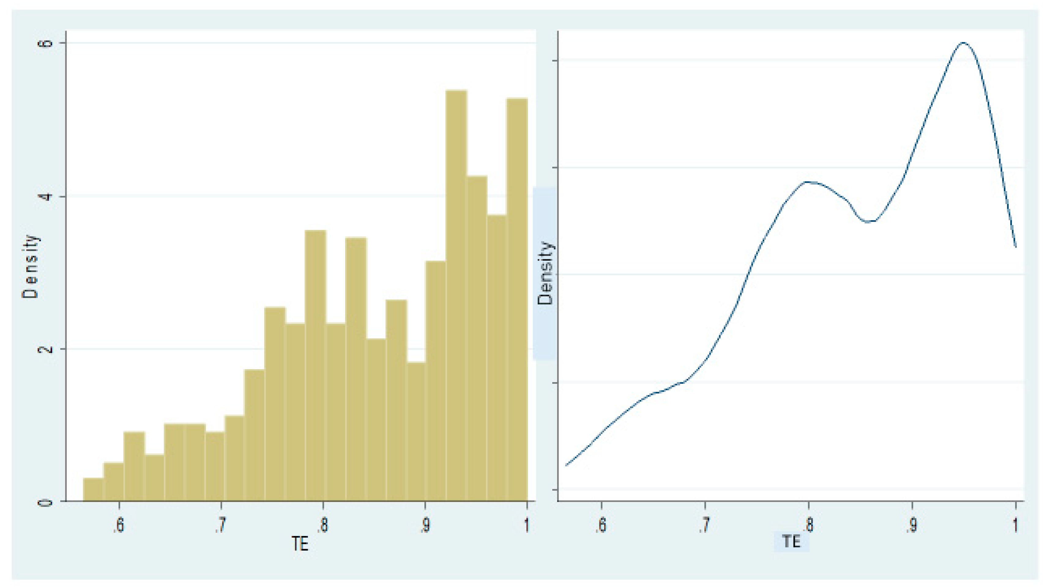
The results in

Table 3. Frequency distribution and summary statistics on overall TE, pure TE, and scale efficiency measures in smallholder groundnut farms.

Efficiency Level	Overall TE		Pure TE		Scale Efficiency
	No. of Farms	Percent	No. of Farms	Percent	No. of Farms	Percent
≤0.60	9	1.89	8	1.68	2	0.42
0.61–0.70	23	4.83	20	4.20	11	2.31
0.71–0.80	62	13.03	54	11.34	23	4.83
0.81–0.90	123	25.84	141	27.52	142	29.83
0.91–0.99	192	40.34	190	39.92	210	44.12
1.00	67	14.08	73	15.34	88	18.49
Total	476	100.00	476	100.00	476	100
Minimum	0.582		0.591		0.638
Maximum	1.000		1.000		1.000
Mean	0.790		0.861		0.932
Median	0.782		0.903		0.989
SD	0.19		0.17		0.09

show that 14 percent of the smallholder farmers have an overall TE of 1.000 (100 percent), with the assumption of CRS. It was also interesting that only around two percent of the total sample farmers fall under the lowest efficiency group—less than 60 percent. This indicates that 84 percent of the sample farms have overall TE scores between 0.61 and 1.00 with respect to use of inputs in groundnut production. The findings further show that overall TE scores ranged between 0.58 and 1.00, with a mean score of 0.79, implying that the sampled groundnut farms could still produce the same level of output, even by reducing 21 percent of the current level of input usage [21,22,23]. As shown in Figure 1, the distribution of overall TE scores is tilted towards the right side, implying a higher level of overall TE in groundnut production, with a mean score of 0.79. The Pure TE scores ranged between 0.59 and 1.000, with a mean score of 0.86, and scale efficiency scores ranged between 0.638 and 1.000, with a mean efficiency score of 0.93. These findings indicate the following:

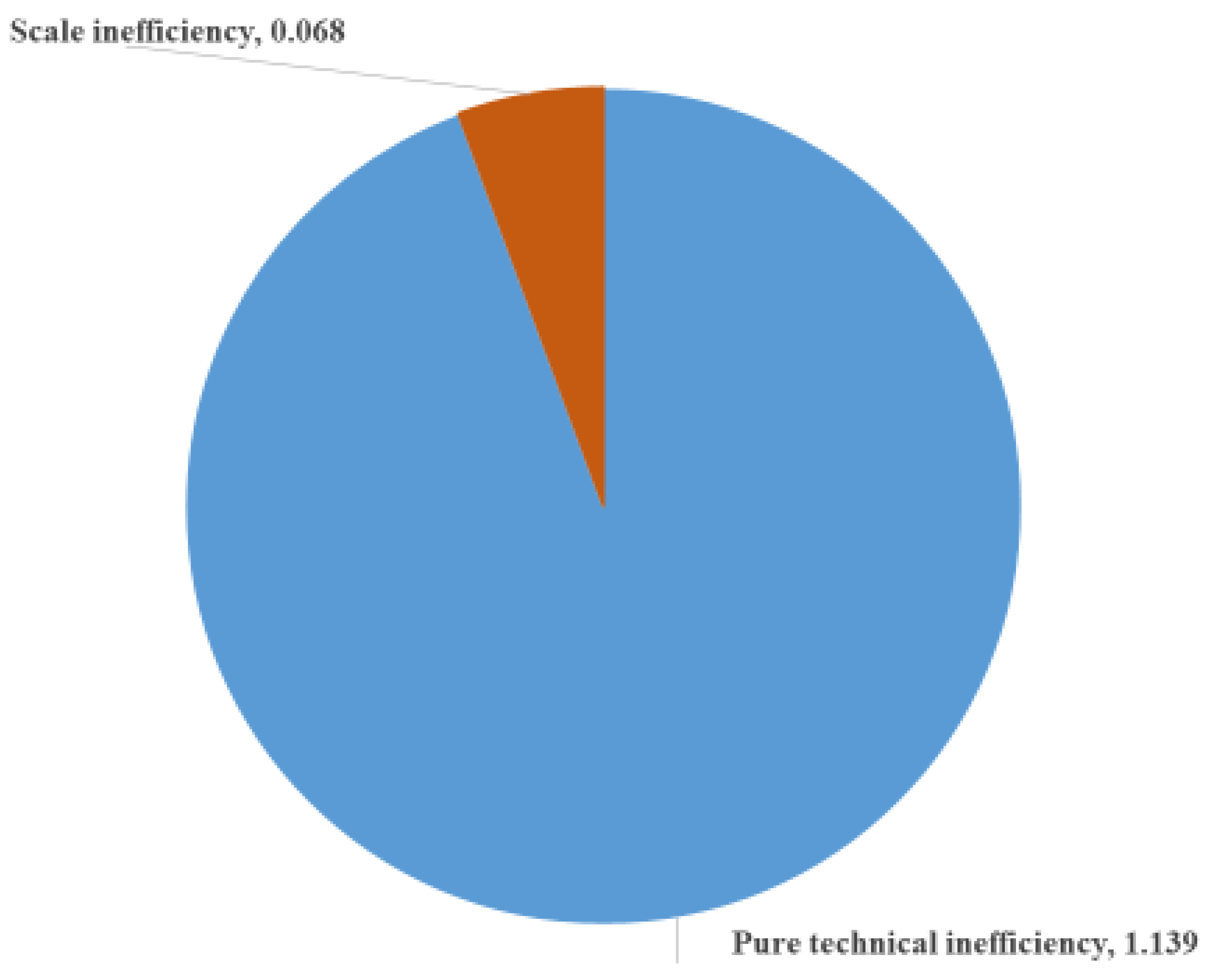
• the splitting of overall TE measure produced estimates of 14 percent pure technical inefficiency and seven percent scale inefficiency (Figure 2);
• by eliminating scale inefficiency, the farms can increase their average overall TE from 0.790 to 0.861;
• the higher scale efficiency of 0.932 indicates that the majority of the groundnut farms are operating at or near to their optimal size;
• the overall technical inefficiency of groundnut farms by 21 percent implies that the farmers are not able to obtain optimal output from the given level of inputs available to them, and they are not utilizing the available inputs efficiently. The overall TE scores can be improved by adopting GAPs among groundnut farms.

4.2.3. Scale of Operations in the Production Frontier

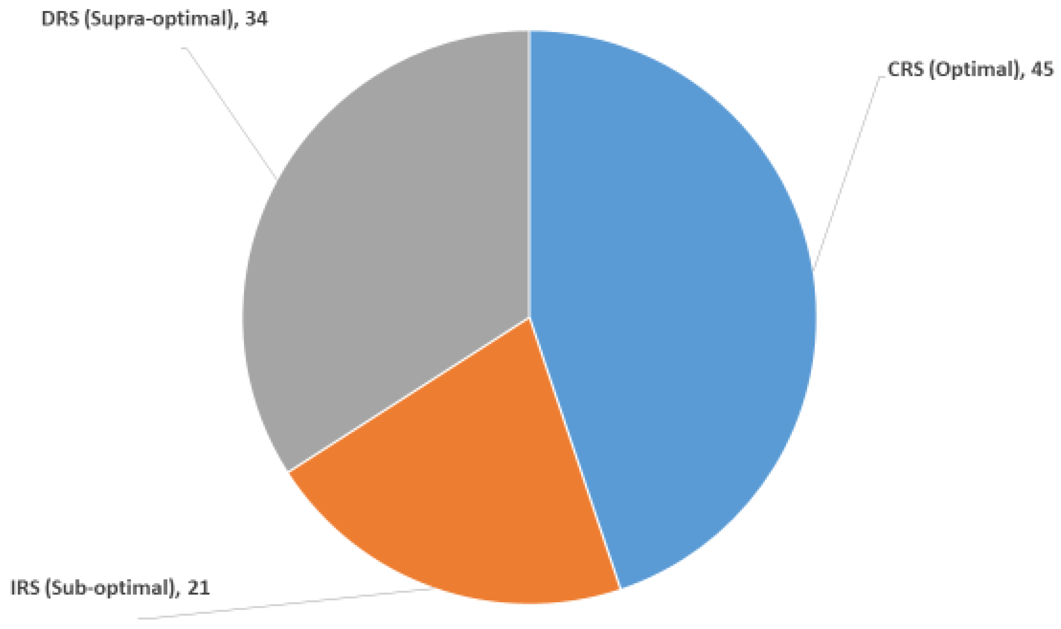
Around 45 percent of the sampled groundnut farmers are operating at optimal scale (CRS) conditions (

Table 4. Summary of RTS results (n = 476).

Characteristics	No. of Farms	Mean Farm Size (ha)	Mean Output (Tonnes)
CRS (Optimal)	213 (44.75)	1.73	3.61
DRS (Supra-optimal)	162 (34.03)	1.58	3.18
IRS (Sub-optimal)	101 (21.22)	1.23	2.69

Note: Figures in parentheses are percent to total.

and Figure 3). However, 21 percent of the farmers are operating at sub-optimal scale (IRS) conditions, and the remaining 34 percent of the farmers are operating at supra-optimal scale (DRS) conditions. The results of the distribution of farmers across IRS and DRS operations in the production frontier revealed that 21 percent of them had the scope to increase the scale size and 34 percent had the scope to reduce the scale size, so as to improve their resource use efficiency [21]. However, a higher mean scale efficiency (0.932) implies that the inefficiency across IRS and DRS farms was mainly because of improper scale size.

4.2.4. Input Slacks and Excess Input Usage

It was found that input slacks, in terms of number of farms, is highest with respect to NPK fertilizers (20%), followed by seed rate (17%), gypsum (11%), and organic manure (6%). This implies that the respective sample farms could reduce the use of these inputs without affecting their output level (

Table 5. Input slacks and number of farms using excess inputs.

Inputs	No. of Farms	% of Total Farms	Mean Input Slack	Mean Input Used	Excess Input Use in Percent
Fertilizer Use (NPK) (kg/ha)	97	20.38	16.58	410.58	4.04
Seed rate (kg/ha)	81	17.02	12.59	154.27	8.16
Gypsum (kg/ha)	52	10.92	9.12	580.16	1.57
Organic manure (t/ha)	29	6.09	0.96	9.35	10.27

). In terms of inputs usage, the mean input slack was found to be highest for NPK fertilizers (16.58 kg/ha), followed by seed rate (12.59 kg/ha), gypsum (9.12 kg/ha), and organic manure (0.96 t/ha), indicating that the sampled groundnut farms are applying higher doses of these inputs. Accordingly, the farms should reduce the doses of these inputs, namely NPK fertilizers, seed rate, gypsum, and organic manure by 4.04, 8.16, 1.57, and 10.27 percent, respectively, with respect to the corresponding values of mean input slacks, and retain the same level of output in terms of production.

4.3. Impact of WBCIS Participation on TE of Groundnut Farms

In the context of frequent weather risks and climate change in Ananthapuramu, participation of farmers in the WBCIS is pivotal for boosting the TE of groundnut farms. Accordingly, to analyze the impact of participation of farmers in WBCIS on the TE of groundnut production, the PSM technique was employed.

Through the PSM technique, the Common Support Condition (CSC) was derived and was found to be satisfactory, in the region of 0.0419 to 0.8568, with a mean of 0.3117 (

Table 6. Estimated propensity scores.

	Percentiles	Smallest
1%	0.0516	0.0419
5%	0.0832	0.0429
10%	0.1100	0.0479	Obs	455
25%	0.1946	0.0506
50%	0.2995		Mean	0.3117
		Largest	Std. Dev.	0.1507
75%	0.4094	0.6633
90%	0.5222	0.6633	Variance	0.0227
95%	0.5723	0.7085	Skewness	0.2989
99%	0.6557	0.8568	Kurtosis	2.525

). This implies that the farmers with the estimated propensity scores in the above range are only considered for this matching exercise and, accordingly, 21 untreated farmers were discarded from the analysis.

It is interesting to note that, before matching, for half of the selected covariates, viz., LHS, GAP, and FE (

Table 7. Testing of covariates balance for treated and untreated.

Variable	Unmatched/ Matched	Mean		% Bias	% Reduction in Bias [100(1-(BiasAM/BiasBM))]	‘t’ test
		Treated	Untreated			tcal	p > |t|
AGE	Unmatched	52.407	51.169	10.8		1.13	0.260
	Matched	52.407	52.073	2.9	73.1	0.25	0.803
LHS	Unmatched	3.6567	3.1271	55.7		5.51 ***	0.000
	Matched	3.6567	3.6267	3.2	94.3	0.31	0.759
EDU	Unmatched	4.2267	4.2457	−0.4		−0.04	0.967
	Matched	4.2267	4.1467	1.6	−320.0	0.13	0.893
GAPs	Unmatched	0.58	0.843	−40.2		−3.81 ***	0.000
	Matched	0.58	0.66	−12.2	69.6	−1.18	0.238
FE	Unmatched	30.687	26.331	38.3		3.98 ***	0.000
	Matched	30.687	31.2	−4.5	88.2	−0.38	0.701
TIME	Unmatched	1.8733	1.8343	5.6		0.55	0.579
	Matched	1.8733	1.76	16.3	−190.2	1.47	0.141

Note: *** = p ≤ 0.01.

) pscore estimates were found to be significant. However, after matching, the pscore estimates of all the covariates were found to be non-significant. Further, the absolute values of unmatched bias reduction ranged from 0.4 to 55.7 percent (Column 5), and after matching, the same ranged from 1.6 to 16.3 percent, and the t_cal values turned insignificant, indicating that all the covariates are now balanced in the model.

The NNM, KBM, and RM methods were employed to estimate the ATT and ATE for indicating the impact of the WBCIS on the TE of groundnut production. The analytical findings (

Table 8. Average impact estimates of PSM on the TE of groundnut production using three matching methods.

Outcome	Sample	Treated	Untreated	Difference	SE	t-Stat
NNM	Unmatched	0.8850	0.7367	0.1483 ***	0.0092	16.07
	ATT	0.8850	0.7294	0.1557 ***	0.0131	11.91
	ATU	0.7367	0.8925	0.1559
	ATE			0.1558
KBM	Unmatched	0.8850	0.7367	0.1483 ***	0.0092	16.07
	ATT	0.8848	0.7308	0.1539 ***	0.0094	16.4
	ATU	0.7367	0.8903	0.1536
	ATE			0.1537
RM	Unmatched	0.8850	0.7367	0.1483 ***	0.0092	16.07
	ATT	0.8860	0.7313	0.1548 ***	0.0091	17.13
	ATU	0.7344	0.8894	0.1549
	ATE			0.1549

Note: *** = p ≤ 0.01.

) revealed that, for the treated farmers, there is a positive and significant increase in the TE of groundnut production compared to untreated counterpart. The ATT of the treated over untreated was comparatively increased by 21.34 percent in NNM, 21.06 percent in KBM, and 21.16 percent in RM, indicating that participation of farmers in the WBCIS has improved their TE by 21.06 to 21.34 percent [24]. The ATE of any randomly chosen farmer was found to be 0.1548 (average of three matching methods), and this implies that if any smallholder groundnut farmer in the district participates in the WBCIS, the TE will increase by 0.1548. Therefore, considerable attention should be given to the promotion of the WBCIS to boost the TE of smallholder groundnut farmers in the district.

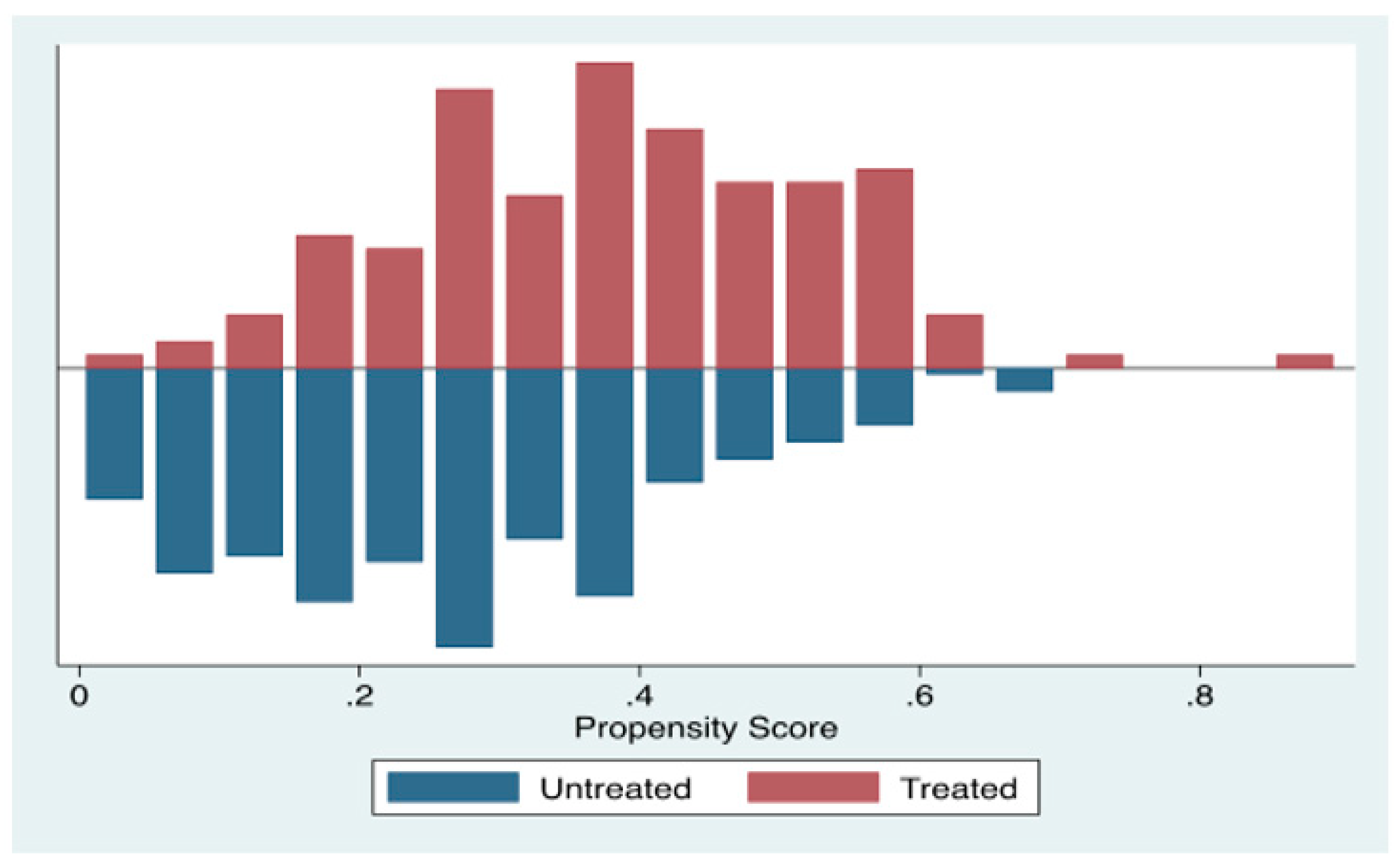
Low Pseudo-R² and the insignificant likelihood ratio tests have proven that both groups have the same distribution in the outcome variables after matching (

Table 9. PSM quality indicators before and after matching.

Indicators	Before Matching	After Matching
Pseudo-R2	0.105	0.016
LR chi2	64.15	6.68
P > chi2	0.000	0.351
Mean Absolute Bias	25.2	6.8
Med Bias	24.5	13.8

). Further, the mean absolute bias after matching is found to be less than 20 percent, and this also proved that the matching procedure balanced the characteristics, in both the treated and the untreated groups, and the same was shown through a common support graph (Figure 4). As the outcome variable, TE still remained significant at different levels of gamma; the Rosenbaum sensitivity test (

Table 10. Rosenbaum sensitivity test for upper bound significance level (N = 159 matched pairs).

Outcome Variable	Gamma *	Significance Level		Hodges–Lehmann Point Estimate		Confidence Interval (95%)
		Upper Bound	Lower Bound	Upper Bound	Lower Bound	Upper Bound	Lower Bound
TE	Γ = 1	0	0	0.1615	0.1615	0.14	0.1835
	Γ = 2	2.70 × 10−11	0	0.1225	0.202	0.098	0.2245
	Γ = 3	1.70 × 10−7	0	0.099	0.2235	0.0725	0.2465
	Γ = 4	0.000014	0	0.083	0.2375	0.055	0.261
	Γ = 5	0.000195	0	0.0715	0.2475	0.0415	0.2715

Note: * gamma—log odds of differential assignment due to unobserved factors.

) revealed that the estimated TEs are robust to unobserved characteristics [19,20,25].

5. Summary and Conclusions

High volatility of rainfall and frequent droughts are the major factors that affect groundnut production among smallholder farmers in the Ananthapuramu district in the context of climate change. Therefore, the management of the above bio-climatic risks is imperative in the context of improving the TE of groundnut production to sustain the livelihoods of smallholder farmers. From this perspective, the WBCIS implemented by the Government of Andhra Pradesh in Kharif, 2007, deserves a special mention in terms of targeting smallholder farmers, especially in severely drought-prone areas such as Ananthapuramu. In this paper, the impact of the participation of smallholder farmers in the WBCIS on the TE of groundnut production was studied in the context of climate change. The findings of DEA revealed that the mean overall TE of sample farms was 0.790, indicating a high level of efficiency in groundnut production. The distribution of scale of operations in the production frontier revealed that 21 percent of the farmers operate at IRS and 34 percent operate at DRS. The estimated impact of WBCIS on the TE of groundnut production revealed that treated farmers enjoy higher ATT compared to their untreated counterpart, as revealed through three matching methods. The ATE was found to be 0.1548 (average of three matching methods). Therefore, the participation of smallholder farmers in the WBCIS has shown a positive impact on the TE of groundnut production. Though the WBCIS insures farmers against weather-related risks, it is yet to gain popularity in the Ananthapuramu district. This is due to complex procedural formalities to participate, the technical challenges involved in designing the indices for various weather parameters, and the fact that the scheme covers only weather related risks and payments are made only for adverse weather deviations, rather than shortfall in yields (being not an yield-guarantee insurance scheme). Further, the scheme demands 25-year rainfall and weather data of each village to create a baseline [1]. Another grey area is the likely difference in rainfall and weather data between the weather station location and the farmer’s field. Therefore, for the success of this scheme, every village should have a weather station to reasonably minimize the discrepancies, which would require almost doubling the existing number of weather stations. Two major reasons that may have led to a sharp decline in WBCIS enrollment in recent years are, firstly, that weather insurance has been made optional and, secondly, a higher premium subsidy is to be borne by the State Government (due to a paucity of Central Government funds). Further, farmers who have access to canal irrigation (head and middle reaches), bore well, and other inputs avoid paying premiums. [1]. In view of this, the following prioritized options must be looked into to encourage the smallholder farmers’ participation in the WBCIS and to ensure their sustainability perspective in groundnut production in Ananthapuramu:

• greater awareness and understanding about the WBCIS among farmers;
• better location of weather stations;
• coverage of more weather parameters or more perils;
• refining the design of the WBCIS (shorter claim settlement periods, greater transparency, and ease of enrollment);
• premium refund for successive no claims.

Above all, strengthening the extension services to disseminate modern crop production technologies, capacity building on GAPs, improving the supply mechanism of quality inputs in good time, and planning for long-term drought-proofing measures to help farmers better adapt to weather shocks and sustain their production and income should be programmatic priorities. Further, in view of the positive influence of the WBCIS on the TE of groundnut farms, it is imperative to promote the same in Ananthapuramu. Therefore, refining the existing scheme with a ‘Farmer-Centered’ approach deserve special mention. It is important to educate and train farmers so they understand that the ‘payment of premium’ to participate in the WBCIS as one of the working capital expenses they incur in the crop production program. In the context of enhancing the TE of resources, it is equally important to give discounts in premiums for farmers participating in the WBCIS if they practice organic farming; integrated pest management; integrated nutrient management; and integrated water resources management, and if they cultivate drought resistant crops; maintain clean bunds without weed infestation; carry out proper maintenance of irrigation and drainage channels; and maintain soils with good pH, EC, and organic carbon etc.

References

- Agricultural Research Station (ARS); Ananthapuramu, Acharya NG Ranga Agricultural University (ANGRAU), Guntur, India. Personal communication, 2020.
- Nair, R. Crop Insurance in India: Changes and Challenges. Econ. Political Weekly 2010, 45, 19–22. [Google Scholar]
- Chetaille, A.; Lagrande, D. L’assurance Indicielle, une Réponse Face aux Risques Climatiques? Available online: https://www.inter-reseaux.org/wp-content/uploads/pdf_p20_21_Gret.pdf (accessed on 3 April 2021).
- Hazell, P.; Anderson, J.; Balzer, N.; Hastrup Clemmensen, A.; Hess, U.; Rispoli, F. L’assurance Basée sur un Indice Climatique: Potentiel D’expansion et de Durabilité pour l’agriculture et les Moyens de Subsistance en Milieu Rural. Available online: https://www.findevgateway.org/fr/paper/2010/01/lassurance-basee-sur-un-indice-climatique-potentiel-dexpansion-et-de-durabilite-pour (accessed on 2 February 2021).
- Burke, M.; de Janvry, A.; Quintero, J. Providing Index–Based Agricultural Insurance to Smallholders: Recent Progress and Future Promise; Documento de Trabajo. CEGA, University of California at Berkeley: Berkeley, CA, USA. 2010. Available online: http://siteresources.worldbank.org/EXTABCDE/Resources/7455676-1292528456380/7626791-1303141641402/7878676-1306270833789/Parallel-Session-5-Alain_de_Janvry.pdf (accessed on 4 April 2020).
- Heimfarth, L.E.; Musshoff, O. Weather index-based insurances for farmers in the North China Plain. Agric. Financ. Rev. 2011, 71, 218–239. [Google Scholar] [CrossRef]
- Clarke, D.J.; Clarke, D.; Mahul, O.; Rao, K.N.; Verma, N. Weather Based Crop Insurance in India. Available online: https://www.researchgate.net/publication/254073298_Weather_based_crop_insurance_in_India (accessed on 31 March 2021).
- Carter, M.; de Janvry, A.; Sadoulet, E.; Sarris, A. Index-Based Weather Insurance for Developing Countries: A Review of Evidence and a Set of Propositions for Up-Scaling. Available online: https://econpapers.repec.org/paper/fdiwpaper/1800.htm (accessed on 6 June 2021).
- Agricultural Statistics at a Glance 2019. Available online: https://eands.dacnet.nic.in/PDF/At%20a%20Glance%202019%20Eng.pdf (accessed on 1 May 2021).
- Narain, S.; Ghosh, P.; Saxena, N.; Parikh, J.; Soni, P. Climate Change—Perspectives from India. Available online: https://ruralindiaonline.org/en/library/resource/climate-change-perspectives-from-india/ (accessed on 3 June 2021).
- Handbook of Statistics, Ananthapuramu; Various Issues; Government of Andhra Pradesh: Ananthapuramu, India, 2019.
- Banker, R.D.; Charnes, A.; Cooper, W.W. Some Models for Estimating Technical and Scale Inefficiencies in Data Envelopment Analysis. Manag. Sci. 1984, 30, 1078–1092. [Google Scholar] [CrossRef] [Green Version]
- Charnes, A.; Cooper, W.W.; Rhodes, E. Measuring the efficiency of decision making units. Eur. J. Oper. Res. 1978, 2, 429–444. [Google Scholar] [CrossRef]
- Pradhan, A.K. Measuring Technical Efficiency in Rice Productivity Using Data Envelopment Analysis: A Study of Odisha. Int. J. Rural. Manag. 2018, 14, 1–21. [Google Scholar] [CrossRef] [Green Version]
- Greene, W.H. Econometric Analysis, 5th ed.; Prentice Hall: Upper Saddle River, NJ, USA, 2003. [Google Scholar]
- Verbeek, M. A Guide to Modern Econometrics, 3rd ed.; John Wiley & Sons: Chichester, UK, 2008. [Google Scholar]
- Willy, D.K.; Zhunusova, E.; Holm-Müller, K. Estimating the joint effect of multiple soil conservation practices: A case study of smallholder farmers in the Lake Naivasha basin, Kenya. Land Use Policy 2014, 39, 177–187. [Google Scholar] [CrossRef]
- Ali, A.; Erenstein, O. Assessing farmer use of climate change adaptation practices and impacts on food security and poverty in Pakistan. Clim. Risk Manag. 2017, 16, 183–194. [Google Scholar] [CrossRef]
- Rosenbaum, P.R. Overt Bias in Observational Studies. In Observational Studies; Springer: New York, NY, USA, 2002; pp. 71–104. [Google Scholar]
- Rosenbaum, P.R.; Rubin, D.B. The central role of the propensity score in observational studies for causal effects. Biometrika 1983, 70, 41–55. [Google Scholar] [CrossRef]
- Tipi, T.; Yildiz, N.; Nargeleçekenler, M.; Çetin, B. Measuring the technical efficiency and determinants of efficiency of rice (Oryza sativa) farms in Marmara region, Turkey. N. Z. J. Crop. Hortic. Sci. 2009, 37, 121–129. [Google Scholar] [CrossRef] [Green Version]
- Simar, L.; Wilson, P.W. Two-stage DEA: Caveat emptor. J. Product. Anal. 2011, 36, 205–218. [Google Scholar] [CrossRef]
- Toma, P. Size and productivity: A conditional approach for Italian pharmaceutical sector. J. Prod. Anal. 2020, 54, 1–12. [Google Scholar] [CrossRef]
- Adebayo, O.; Bolarin, O.; Oyewale, A.; Kehinde, O. Impact of irrigation technology use on crop yield, crop income and household food security in Nigeria: A treatment effect approach. AIMS Agric. Food 2018, 3, 154–171. [Google Scholar] [CrossRef]
- Becker, S.O.; Caliendo, M. Sensitivity Analysis for Average Treatment Effects. Stata J. 2007, 7, 71–83. [Google Scholar] [CrossRef] [Green Version]
Figure 1.
Distribution of TE scores among smallholder groundnut farms.
Figure 2.
Pure technical inefficiency and scale inefficiency among groundnut farms.
Figure 3.
Distribution (%) of scale of operations of groundnut farms.
Figure 4.
Propensity score distribution and common support.