

Abstract
Afforestation and reforestation have the potential to provide effective climate mitigation through forest carbon sequestration. Strategic reforestation activities, which account for both carbon sequestration potential (CSP) and economic opportunity, can provide attractive options for policymakers who must manage competing social and environmental goals. In particular, forest carbon pricing can incentivize reforestation on private land, but this may require landholders to forego other profits. Here, we utilize an ambitious geospatial approach to quantify economic opportunities for reforestation in the state of Maryland (USA) based on high-resolution remoting sensing, ecosystem modeling, and economic analysis. Our results identify spatially-explicit areas of economic opportunity where the potential revenue from forest carbon outcompetes the expected profit of existing cropland at the hectare scale. Specifically, we find that under a baseline economic scenario of $20 per ton of carbon (5% rental rate) and decadal average crop profitability, a transition to forest on agricultural land would be more profitable than 23.2% of cropland in Maryland under a 20 year land-use commitment. Accounting for variations in carbon and crop pricing, 5.5%–55.4% of cropland would be immediately outcompeted by expected forest carbon revenue, with the potential for an additional 0.5%–10.6% of outcompeted cropland within 20 years. Under the baseline economic scenario, an annual allocation of $5.8 million towards a carbon rental program could protect 6.93 Tg C (3.4% of the state's total remaining CSP) on reforested croplands. This moderate yearly cost is equal to 9.7% of Maryland's average annual auction proceeds from participation in the Regional Greenhouse Gas Initiative (between 2014 and 2018), and 19.3% of the average annual subsidy payments for corn, soy, and wheat allocated over the same period. This methodological approach may be useful for state governments, not-for-profit organizations, or regional climate initiatives interested in identifying strategic areas for reforestation.
Export citation and abstract BibTeX RIS

Original content from this work may be used under the terms of the Creative Commons Attribution 4.0 license. Any further distribution of this work must maintain attribution to the author(s) and the title of the work, journal citation and DOI.
1. Introduction
Forests are important ecosystems that provide a broad range of ecosystem services, including carbon storage and climate change mitigation. In this context, multiple national and international commitments have been launched to not only protect forests (e.g. REDD+) but also to restore them. In early 2019, the United Nations Environmental Programme and Food and Agriculture Organization launched the 'Decade of Ecosystem Restoration 2021–2030' recognizing a global window of opportunity for forest restoration to offset serious concerns around climate change and biodiversity loss (UNEP 2019). In mid-2020, the World Economic Forum launched the One Trillion Trees initiative (1t.org), designed to support the UN Decade on Ecosystem Restoration with a platform for connecting leading governments, businesses, civil society, and ecopreneurs committed to conserving, restoring, and growing one trillion trees globally. Strategic afforestation and reforestation activities, which account for both carbon sequestration potential (CSP) and co-benefits such as economic opportunity, can provide attractive options for policymakers who must manage competing social and environmental goals (Jackson and Baker 2010).
To economically incentivize reforestation, forest carbon payments, which compensate landowners for growing trees on their land, have traditionally been envisioned and applied either in the form of carbon rental policies (Lintunen et al 2016) or carbon compensations policies such as subsidies and taxes (Daigneault et al 2020). While there are benefits to both approaches, rental policies are considered more politically and economically expedient as the money transfers are always from the administrator to the forest owner (Lintunen et al 2016). At minimum, rental policies include a carbon price to estimate the overall monetary value of a forest carbon stock, a specific rate at which the value of this stock is annually rented, and a fixed agreement period during which the landowner agrees to maintain regrowing forests. Carbon rental fees provide an opportunity to compensate individual landowners for the social benefit sequestered carbon provides while incentivizing landowners to maximize standing biomass and avoid intentional reversal of tree cover throughout a long-term renewable contract (Evans et al 2018).
While many land-use types may remain economically competitive under a forest carbon price, potential competition with agricultural land is of particular interest (e.g. Smith et al 2013). Although some US states have worked to prevent the conversion of prime agricultural land to other land-uses (particularly development), there may also be a unique potential to maximize the reforestation of marginal lands, areas where field crops maintain low productivity due to erosion or other environmental risks when cultivated (e.g. Gelfand et al 2013, Kang et al 2013). Natural forest regeneration on agricultural land also represents a 'distinct ecological, social and policy context' and requires specific analysis that contrasts with that more regularly provided in studies 'targeting selective logging and associated silvicultural treatments in natural forests managed for timber production' (Chazdon et al 2020). Specifically, assessing the potential competition of reforestation on agricultural land will require detailed information on the amount of carbon capable of being sequestered on a given land parcel, the profitability of this sequestration under different rental scenarios, and how this potential revenue compares to the likely profit generated if the land were to remain cropland.
Interest in the economic implications of a forest-based carbon policy in the U.S. has expanded in recent years. However, much of this work focuses on national land-use dynamics (e.g. Lubowski et al 2006, Monge et al 2016), evaluates opportunity costs with course estimates of carbon uptake (e.g. Nielsen et al 2014), targets implications for commercial timber harvest (e.g. Daigneault et al 2010, Nepal et al 2013), or relies primarily on sector optimization and stand-level models (e.g. Sohngen and Mendelsohn 2003, Pohjola et al 2018). Among the remaining research gaps are knowledge limitations about specific locations for potential natural forest regeneration on agricultural land, how long it will take to deliver specific related environmental and social outcomes, and robust economic projections to evaluate the impact of natural regeneration on local livelihoods (Uriarte and Chazdon 2016, Ding et al 2017, Chazdon et al 2020).
Recent advances in high-resolution remote sensing and ecosystem modeling provide an opportunity to more precisely and dynamically address these research gaps by enabling improved estimation of economic tradeoffs associated with reforestation across space and time. In particular, 3D structure information on vegetation acquired from lidar remote sensing has provided by far the most accurate forest estimates across broad geographical extents (e.g. Dubayah and Drake 2000, Dubayah et al 2010). High-resolution carbon maps (∼30 m) have been generated from airborne lidar data at county, state, and regional levels (Huang et al 2015, 2019, Tang et al 2021), and spaceborne missions (e.g. NASA GEDI and ICESat-2) are improving our knowledge of global carbon stocks by providing near-global 1 km gridded estimates of forest canopy height, vertical canopy structure, and surface elevation (Dubayah et al 2020). Moving from current forest conditions to CSP, NASA Carbon Monitoring System (CMS) projects are utilizing this remote sensing data (optical and LiDAR), coupled with prognostic ecosystem modeling and existing field observation systems, to project forest CSPs at high spatial resolution (e.g. Hurtt et al 2019, Ma et al 2021). Since the resolution of these products is 90 m, more than 100 000 times that of many global vegetation models, it is now possible to project sequestration outcomes at fine spatial scales. This has many potential applications for land-use planning. In particular, these products can reveal the spatial heterogeneity of CSP and clarify the time required to achieve it.
Here, we use high-resolution NASA CMS forest carbon products for Maryland (USA) to quantify and map the economic potential of reforestation relative to cropland profit under a carbon pricing system. To estimate the economic opportunity provided by reforestation, we use a rental economic model, which includes an annual rental rate as a function of carbon price. To understand the land-use implications of this system, we evaluate (a) where the economic opportunity for reforestation is highest across the state, (b) how carbon price and rental rate influence the amount of cropland area that becomes outcompeted by expected forest carbon revenue, (c) the year at which projected forest carbon revenue outcompetes expected cropland profit at the landowner scale, and (d) the impact of agreement length on overall competition. We also consider the amount of carbon likely to be sequestered and the cost of implementing such a program via individual land-use agreements under a range of economic scenarios. We apply an ambitious geospatial approach to demonstrate that the spatial and temporal heterogeneity of CSPs can be combined with economic data to support strategic land-use planning at the state and county levels. This work goes beyond previous studies because it explicitly considers dynamic annual estimates of aboveground biomass and subsequent land-use competition at 90 m resolution, which allows us to answer more targeted questions about how much forest carbon can be stored in which areas and by when.
2. Data and methods
2.1. Study area
The state of Maryland (USA) provides an excellent study area for this prototype project due to its land-use history and strong climate mitigation goals. The dominant potential vegetation type for the state is deciduous forest (Ramankutty and Foley 1999). Due to widespread human-induced land cover and land-use change, the landscape is characterized by fragmented forests with restoration opportunities. Depending on forest definition and method, forest covers 33%–41% of the land area and croplands account for 32% (Jin et al 2013, Lister and Widann 2016). As with the majority of the US Eastern seaboard, 90% of Maryland was cleared of forest and converted to agriculture by the mid-19th century. These lands were converted partially back to forest in the early 20th century as agriculture's economic importance declined in the state. Significant quantities of forest were subsequently lost to development in the mid to late 20th century.
Currently, Maryland has legislation related to forestry and climate mitigation that actively inform land-use planning. The Forest Conservation Act was enacted in 1992 and strengthened in 2013 with the intent for 'no-net-loss' of forests and to maintain forest cover above 40% in Maryland. The Greenhouse Gas Reduction Act (GGRA) was passed in 2009, directing the state to reduce climate pollution 25% by 2020 and create a Greenhouse Gas Reduction Plan. In 2016, the GGRA was reauthorized and strengthened to a 40% reduction by 2030, requiring an updated plan with improved reforestation goals. The final 2030 plan was released in February 2021 with a focus on improving the carbon management of farms and forests (MDE 2021). As a member of the US Climate Alliance, Maryland has also participated in the Natural and Working Lands (NWL) Challenge, which commits states to maintain NWLs as a net carbon sink (USCA 2020).
2.2. NASA carbon monitoring system products
The foundational forest carbon sequestration products for this study were derived from the Ecosystem Demography model (ED) (Moorcroft et al 2001, Hurtt et al 2004), and previously published in Hurtt et al (2019) as part of the NASA CMS (supplement, available online at stacks.iop.org/ERL/16/084012/mmedia). Here, the forested fraction of every 90 m grid cell is estimated circa 2011 using statewide airborne lidar and NAIP optical imagery (O'Neil-Dunne 2019). The forested fraction is then held constant throughout the model projection such that the biomass density in any 90 m grid cell over time is the area-weighted sum of carbon accumulated on contemporary forest area, and forest carbon accumulated on previously non-forested areas (e.g. via reforestation). ED assumes all reforestation occurs via natural regeneration with native plant functional types. Following definitions in Hurtt et al (2019), carbon sequestration potential (CSP) is defined as 95% of the maximum aboveground biomass a site reaches during forest succession. In computing these potentials, all non-forest area could theoretically be reforested, excluding wetland and impervious surface. The CSP gap is defined as the difference between CSP and current carbon stocks (aboveground biomass (AGB)). Modeled successional pathways can take upwards of 500 years to complete (i.e. reach CSP), but in this study, we focus on AGB growth trajectories through 2100, as this is a more policy- and landowner-relevant period.
2.3. Land cover and ownership
To understand existing spatial patterns of land-use, all 90 m carbon sequestration data layers were stratified by land use classifications to identify those with the largest carbon stocks and highest CSP. The Maryland Department of Planning provided spatial polygon data (2015/16 edition data) for all property parcels in the state, including attribute data such as zoning and land-use designations (MDP 2020). Zoned agricultural areas can include both annual crops as well as woodland that is either associated with a farm, part of an approved forest plan, or protected within a forest conservation management agreement. Zoned agricultural areas were also classified as private land areas, as they are distinct from tax 'exempt' government-owned properties.
2.4. Crop productivity and profitability
We established a baseline case for crop profitability in Maryland, assuming no annual change in crop productivity (yield), revenue, profit, or spatial distribution of crop type through 2100. First, the grid cell fraction of soybean, wheat, and corn was estimated using the United States Department of Agriculture (USDA) National Agricultural Statistics Service (NASS) Cropland Data Layer (CDL) (USDA NASS 2011). We used 2011 CDL data to match the date of the NASA CMS tree canopy cover product. In this year, wheat, soybean, and corn collectively represented 13.3% (330 031 ha) of Maryland's land area, and just over half of all zoned agricultural land. As CDL categorically assigns crop types at 30 m, we estimated the crop fraction by counting the number of 30 m pixels of soybean, corn, and wheat within the 90 m grid; no 30 m pixel had more than one crop identification. The tree canopy fraction layer was considered dominant, such that in any case where the sum of the tree canopy fraction and the crop cover fraction was greater than one (e.g. greater than 100%), the total crop fraction for each 90 m pixel was reproportioned to equal the difference between the tree canopy fraction and one.
The average productivity of three focus Maryland crops (corn, soy, and wheat), were calculated using information on agricultural yield provided by USDA NASS and Maryland Department of Agriculture (USDA NASS 2019 Maryland Crop Survey Online). Average annual yield data was reported from 2010 to 2019 for all three crop types across 23 counties in Maryland (excepting Baltimore City) in bushels per acre. For each county, we calculated the average decadal yield per crop type. Crop yield was subsequently multiplied by the respective crop fraction within each 90 m pixel and converted from acres to hectares to estimate the total number of bushels per hectare over cropland area. To better account for property-scale variation in productivity that may be obscured by an average county-level yield estimate, the yield in each 90 m pixel was multiplied by the National Commodity Crop Productivity Index (NCCPI) value (range from 0 to 1) in that same grid cell and subsequently divided by the average NCCPI value calculated for the county (figure S1, Dobos et al 2012).
Crop revenue was calculated as a function of crop yield and crop price. Crop pricing data was obtained from the USDA NASS and State of Maryland Annual Agricultural Overview, which provides a single annual market price for corn, soybeans, and wheat in USD per bushel from 2010 to 2019 (USDA NASS 2019). Similar to crop yield data, we calculated the decadal average price for each crop type. Crop revenue was estimated for each 90 m pixel by multiplying the respective crop yield value by the average market price.
Crop profit is equal to crop revenue minus production costs, plus crop subsidies. For all three crops, the total cost per hectare was estimated using the University of Maryland Extension Field Crop Budgets for 2018 (Dill et al 2017). Extension budgets include a range of variable and fixed costs to estimate economic returns at a given yield and market price (tables S1–S3). We held most crop costs constant across space using the Extension Office's default budgets for Roundup Ready Soybeans, Conventional Corn Grain, and Soft Red Winter Wheat. Only yield-dependent variables, such as hauling charges, were adjusted for each grid cell relative to NCCPI-adjusted 90 m yield estimates. Custom charges for field operation costs include charges for equipment, labor, repairs and maintenance, and fuel/lube for that practice.
Average county-level crop subsidies were obtained via the Environmental Working Group (EWG) Farm Subsidy Database (EWG 2018). Subsidy data was reported by crop type and county and comprised four elements: commodity programs, crop insurance subsidies, conservation programs, and disaster programs. We used 2018 data to reflect recent payments under the 2014 Farm Bill (Agricultural Act of 2014). The first year of payments under the 2018 Farm Bill had not yet been released at time of publication. For each crop type, we generated 90 m subsidy payments by first dividing total crop subsidies (USD) in each county over the total number of hectares in production and then multiplying that number by the crop fraction.
2.5. Rental model for forest carbon
The forest carbon rental model in this study includes a carbon price and rental rate that remain temporally constant. Annual carbon rental revenue was quantified and mapped for each 90 m grid cell (e.g. USD/Mg C/ha/yr) by multiplying modeled forest AGB by the rental model (supplement). We considered all forest carbon as eligible for rental, including both trees that existed on the 90 m grid as of 2011 and trees regrowing since 2011 on the remaining non-forest area. The carbon price was set at $20/Mg C in the baseline rental scenario, which is broadly consistent with recent trading prices within the Regional Greenhouse Gas Initiative (RGGI) (i.e. $4–6 per short ton of CO2). The rental rate, which represents the proportion of the total forest carbon stock value rented in any given year, was set for 5%; a level within the range of cropland rental rates across the RGGI domain (USDA NASS 2020). As the ED model projects AGB growth based on unassisted natural forest regeneration, this study assumes an establishment cost of zero (Brancalion et al 2016, Cruz-Alonso et al 2019).
2.6. Land-use competition
Finally, we estimated the locations and years at which projected forest carbon revenue outcompeted expected cropland profit. For each year between 2011 and 2100, we compared the cumulative forest carbon revenue of every 90 m pixel against the cumulative cropland profit expected on that same 90 m pixel (supplement). If there was more than one crop type within the same 90 m grid cell, all crop profits were summed to report a single crop profit value. Where forest carbon revenue exceeded cropland profit, we flagged the pixel as outcompeted and recorded the year this occurred (figure S2). In instances where cropland was immediately outcompeted by forest carbon revenue in 2011, we expected relatively low crop profit and existing trees (e.g. non-zero AGB) within the same 90 m grid. Where forest carbon revenue never outcompeted cropland, we expected very high crop profit such that even as trees grew to maximum potential, total forest carbon revenue would never exceed crop profit under the current rental scenario. This work assumes a discount rate of zero for both cumulative crop profit and cumulative forest carbon revenue (see supplement for further discussion).
2.7. Sensitivity analysis
We tested the sensitivity of these results using multiple carbon rental and crop pricing scenarios. First, we generated 20 carbon rental factors between 0.5 and 10, which represent the product of multiplying a given carbon price by a specific rental rate. A single rental factor can represent multiple price and rate combinations (table S4). Here, a rental factor of 1 represents our baseline carbon rental scenario, where $20/Mg C is multiplied by the 0.05 rental rate. Next, we identified the minimum and maximum market price (USD/bushel) for all crop types over the past decade (2010–2019). We then generated 20 crop pricing scenarios between these bounds with the price of all three crop types increasing or decreasing in the same direction (e.g. with $4.90/$10.04/$5.27 per bushel representing our baseline crop pricing scenario for corn, soybeans, and wheat, respectively). We subsequently re-ran our competition analysis across all 400 economic scenarios (e.g. 20 rental and 20 crop pricing scenarios). Finally, we tested the sensitivity of changing crop subsidies on overall competition in the baseline economic scenario using two bounding cases. In case one, we removed all subsidies, and in case two, we doubled all subsidies.
3. Results
Here we first provide an overview of crop profitability and projected forest carbon revenue across the State of Maryland. We then review the results of the land-use competition analysis across space and over time under our baseline economic scenario. Finally, we discuss the potential spatial, carbon, and economic impacts of changing the economic scenario under a sensitivity analysis. More detail and supporting figures can be found in the supplement.
3.1. Crop productivity and profitability
Under the baseline crop pricing scenario, crop yield, revenue, and profitability varied spatially and by crop type. Crop yield, scaled by soil productivity and adjusted by crop fraction ranged widely for all crop types (figures S4–S6). Crop revenue varied with yield, ranging from $0 to $2690 per 90 m for corn, $0 to $1734 for soy, and $0 to $988 for wheat (figure 1(a)). Geographically, high revenue areas were distributed across the state, with concentrations along the eastern seaboard and Frederick, Carroll, and Washington Counties in north-central Maryland (figures S7–S9(a)). Average crop subsidies ranged from $0 to $100 per 90 m for corn, $0 to $194 for soy, and $0 to $19 536 for wheat (figure 1(b)). The highest wheat subsidies were concentrated in Talbot County, located in southeastern Maryland, while the highest corn and soy subsidies were found in Frederick and Kent Counties, respectively (figures S7–S9(b)). The cost of crop production ranged from $10 to $1340 per 90 m for corn, $7 to $730 for soy, and $11 to $886 for wheat (figure 1(c)), with production costs generally following the spatial pattern of crop revenue (figures S7–S9(c)). Finally, crop profit, a function of revenue, cost, and subsidies, ranged from $623 to $1350 per 90 m for corn, $526 to $1005 for soy, and $635 to $211 for wheat (figure 1(d)). While crop profits were overwhelmingly positive and widely distributed across the state, negative profits were also found throughout, with the highest concentrations in Wicomico (corn), Charles (soy), and Frederick Counties (wheat) (figures S7–S9(d)).
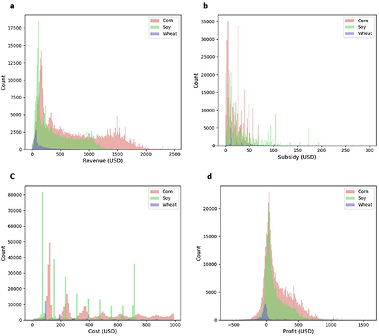
Figure 1. Statewide crop revenue (a), subsidies (b), costs (c) and profit (d) in USD per 90 m under the baseline crop pricing scenario.
Download figure:
Standard image High-resolution image3.2. Forest carbon revenue
With a baseline carbon rental scenario of $20 per ton of carbon and a 5% rental rate, annual revenue from forest conservation and reforestation ranged from $0 to $151 (avg. $43.63) per 90 m over 20 years, with the most profitable land areas representing areas with the highest AGB in any given year. In this way, the spatial pattern of forest carbon revenue followed the spatial heterogeneity of modeled AGB and annual carbon sequestration published in Hurtt et al (2019) (figure S10). After 20 years, projected revenue increased to average annual payments of $65 by 2050, $73 by 2070, and $80 by 2090 (figure 2).

Figure 2. Statewide forest carbon revenue (USD per 90 m) between 2011 and 2110 under the baseline carbon rental scenario.
Download figure:
Standard image High-resolution image3.3. Land-use competition and sensitivity analysis
Under the baseline economic scenario, 22.2% (1273 km2) of cropland was immediately outcompeted by forest carbon revenue (figure 3). With ongoing forest biomass accumulation, outcompeted cropland increased by 1% (52.2 km2) to a total of 23.2% by 2030. Geographically, outcompeted lands were found in every county with the highest concentrations of immediately outcompeted cropland located in southeastern and south-central Maryland (figure 4). If all outcompeted lands were reforested under a 20 year rental agreement, the state could expect to protect 6.9 Tg C at an average annual cost of $5.8 million.
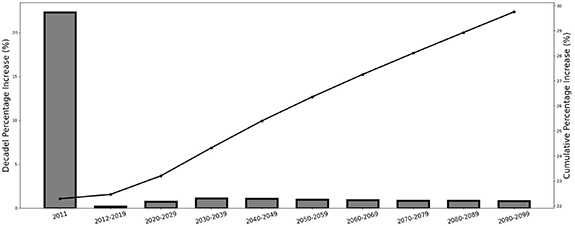
Figure 3. Proportion of Maryland cropland area outcompeted by forest carbon revenue under the baseline economic scenario immediately in 2011, and over each following decade from 2012 to 2100. The bars represent the percent increase in outcompeted cropland over the previous decade, and the solid line represents the cumulative percentage of outcompeted cropland between 2011 and the end of each respective decade.
Download figure:
Standard image High-resolution image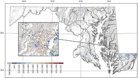
Figure 4. Spatial distribution of outcompeted cropland between 2011–2311 under the baseline economic scenario. Dark blue areas show where cropland is immediately outcompeted. Gray areas highlight cropland areas that remain profitable through 2311 under the baseline scenario. All other colored areas respectively represent the decade within which forest carbon revenue exceeds expected crop profit. The inset provides a closer view of the spatial heterogeneity provided at 90 m resolution.
Download figure:
Standard image High-resolution imageWhen the carbon rental scenario was fixed at the baseline but crop prices were higher than the decadal average, the percentage of immediately outcompeted cropland declined to between 7.3 and 20.3%. Conversely, when crop prices were lower than the decadal average, immediately outcompeted cropland increased to between 24.6% and 44.1% (figure 5). Under lower crop prices, the state could sequester an additional 0.5–4.4 Tg C over the 20 year rental period due to the increase in outcompeted cropland eligible for profitable reforestation. The cost to rent all outcompeted lands increased to between $6.2 and 8.9 million annually (figure 6).
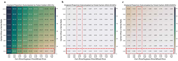
Figure 5. Proportion of Maryland cropland area outcompeted by forest carbon revenue immediately in 2011 (a) and additionally between 2012–2019 (b) and 2020–2029 (c) under a select range of economic scenarios. Where both red boxes intersect is the baseline economic scenario. The vertical dotted box highlights the impact of maintaining the baseline crop pricing scenario but changing the carbon rental scenario. The horizontal dashed box highlights the impact of maintaining the carbon pricing scenario under changing crop pricing scenarios.
Download figure:
Standard image High-resolution image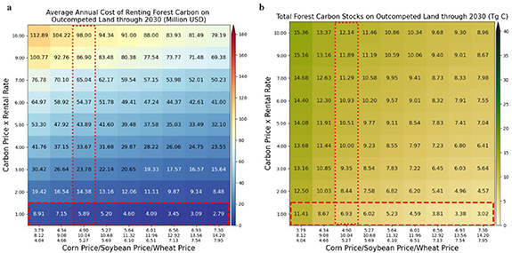
Figure 6. Average annual rental payments for all lands outcompeted by 2030 (a) and the corresponding amount of forest carbon on such lands (Tg C) (b), including the ongoing growth of existing trees and regrowth from new plantings. Where both red boxes intersect is the baseline economic scenario. The vertical dotted box highlights the impact of maintaining the baseline crop pricing scenario but changing the carbon rental scenario. The horizontal dashed box highlights the impact of maintaining the carbon pricing scenario under changing crop pricing scenarios.
Download figure:
Standard image High-resolution image
When crop prices were fixed but the carbon rental factor was higher than the baseline scenario, the percentage of immediately outcompeted cropland increased to between 24.2% and 36.6% (figure 5). An additional 1.9%–7.1% of cropland was outcompeted by 2030. Correspondingly, the increase in outcompeted cropland could result in 7.8–12.1 Tg C sequestered by 2030 (between 12.5% and 175% higher than the baseline scenario), with the total annual cost of such payments increasing to between $9.9 and 98 million (figure 6).
Changing the economic scenario under a 20 year rental agreement produced a wide range of competition, carbon, and rental cost outcomes. The percentage of immediately outcompeted cropland ranged from 5.5% to 55.4%. The cumulative outcompeted cropland ranged from 5.7% to 66.5%. The total amount of carbon sequestered ranged from 2 to 15.3 Tg C at an annual average cost between $910 000 and $112.8 million. Lengthening the rental agreement increased cumulative outcompeted cropland by an additional 0.2%–10.6% (30 years), 0.4%–17.8% (40 years), and 0.6%–23% (50 years) depending on the economic scenario (figure S11). Such changes correspondingly increased the total amount of carbon sequestered and annual average cost to rent it (figure S12).
Under the baseline economic scenario, removing subsidies had a marginal effect on the proportion of outcompeted cropland. Immediately outcompeted lands increased 3.7 percentage points, from 22.6% to 26.3%, with cumulative outcompeted lands increasing an additional 0.9% by 2030 (relative to 0.7% with subsidies) (figure S13). The total amount of carbon protected increased to 7.74 Tg C due to the increase in outcompeted lands and raised the average annual payment cost to $6.4 million (figure S14). Doubling total subsidies decreased immediately outcompeted cropland by a similar magnitude (3.8%), reaching 19.6% of cropland over 20 years (figure S15). The amount of carbon protected declined to 6.23 Tg C with an average annual rental cost of $5.39 million (figure S16).
4. Discussion and conclusions
We demonstrate with an ambitious geospatial approach that the spatial and temporal heterogeneity of CSPs can be combined with economic data to support strategic land-use planning at the state and county levels. Specifically, we find that economic opportunities for forest restoration on cropland do exist across the state, even under a conservative baseline economic scenario. Increasing the carbon rental scenario can make more cropland in the state eligible for profitable reforestation, both immediately and by the end of the rental agreement. However, not all cropland is outcompeted under any economic scenario presented, highlighting the importance of representing economic opportunity as spatially-explicit. Here, the use of high-resolution ecosystem modeling with lidar remote sensing data, has provided an unprecedented opportunity to perform this type of spatial analysis with attention to heterogeneity at the property scale. Utilizing these results, individual landowners can project potential economic profit relative to the carbon rental scenario proposed. Policymakers, interested in incentivizing reforestation to meet state goals, may also be able to use this information to estimate projected program costs and the total amount of forest carbon they are likely to sequester relative to the cropland amount under agreement.
4.1. Impact of economic model variables
Under the baseline economic scenario, the total proportion of cropland outcompeted under a 20 year rental agreement was relatively modest (23.2%), with the vast majority of this cropland immediately outcompeted in 2011 (∼22.6%). Existing mature trees that surround cropland areas as well as negative profits in some regions largely account for this immediate economic benefit (figures S16). This finding suggests that forest conservation is essential for securing competitive revenues at the start of the rental agreement. At the same time, minimal increases in additional outcompeted cropland (∼1%) through the end of the rental period show that for the vast majority of cropland under this pricing scenario, biomass accumulation from newly planted trees does not produce enough additional revenue to outcompete expected crop profit by 2030.
The cost of renting forest carbon on all outcompeted land area under the baseline economic scenario is also relatively modest at $5.89 million annually. However, this is an average annual cost with rental payments generally increasing each year as trees grow. For comparison, these annual rental payments are equivalent to 9.7% of Maryland's average annual auction proceeds ($60.7 million) from participation in the Regional Greenhouse Gas Initiative between 2014 and 2018 (RGGI 2020a), and 19.3% of the average annual subsidy payments for corn, soy, and wheat ($30.5 million) distributed over the same time period (EWG 2018). The total amount of carbon protected under the baseline scenario (6.93 Tg C) is 6.2% of the state's current AGB (110.8 Tg C) and 3.4% of the state's total remaining CSP (204.1 Tg C) (Hurtt et al 2019). While a small fraction of the state's total CSP, 6.93 Tg C is 16 times the amount of carbon (1.5 MMtCO2e) expected to be sequestered by 2030 via state forest management and reforestation activities listed within the Greenhouse Gas Emissions Reduction Act plan (MDE 2021).
Changing the rental scenario under a 20 year rental agreement does impact overall competition. Since the market generally influences crop prices, program managers could strategically select a competitive carbon rental scenario to estimate the total amount of outcompeted cropland as well the upper bound of expected carbon sequestration relative to the cost. For example, under decadal low crop prices, revenues generated from a carbon price of $100 Mg C−1 with a rental rate of 10% (e.g. a rental factor of 10) could immediately outcompete 55.4% (3166 km2) of cropland area (a 32.2% increase from the baseline scenario). Correspondingly, the carbon sequestered could increase to upwards of 12.1 Tg C (almost double that of the baseline scenario). For any scenario, the projected amount of carbon sequestered and the corresponding cost to protect it is contingent on all outcompeted land being reforested under rental agreements. If only a subsection of this land is enrolled, the corresponding amount of carbon and related rental costs will be smaller. Because the NASA CMS forest carbon products used in this study are spatially explicit, it is possible to estimate the projected rental payments and carbon sequestered for any subset of cropland selected.
Changing the agreement's length had a greater effect on the total amount of carbon stored than the percentage of cropland outcompeted. For example, under the baseline scenario, the percentage of outcompeted cropland increased an additional ∼1% each decade from 2030 to 2060, but the total amount of carbon increased ∼17% over the same time period. Under a very high carbon rental factor, outcompeted cropland would increase an additional ∼7.6% per decade from 2030 to 2060, with the total amount of carbon sequestered increasing an average of 28% per decade. These trajectories suggest that a longer land-use agreement, especially under a higher rental scenario, may make the transition to forestland more economically advantageous for a small percentage of farmers. However, the real benefit of a longer rental agreement may be the amount of carbon likely to be sequestered.
Finally, while crop subsidies are assumed to influence greatly overall crop profitability in the United States, our results suggest they have only a small effect on overall competition. When subsidies were eliminated, the proportion of outcompeted cropland only increased by 3.7% under a 20 year rental agreement. This suggests that overall crop revenue under the baseline crop pricing scenario is still relatively competitive compared to expected forest carbon revenue. Doubling the subsidy decreased the proportion of outcompeted cropland by a similar magnitude. While our analysis assumed subsidy payments were distributed proportionally across all cropland, in reality subsidy payments are often distributed to a small number of recipients. For example, according to the 2017 USDA Census of Agriculture, only 28.7% of all Maryland farms received government subsidies with the average farm receiving $12 471 annually (USDA 2019). While the USDA does not report the number of cropland hectares owned or managed by subsidy recipients, they do report the average farm size in Maryland (160 acres). For comparison, a 160-acre farm receiving $77.94 per acre ($192.75 ha−1) in annual subsidy payments (based on a $12 471 total) would fall in the middle of our baseline estimates, where subsidy payments reach nearly $350 ha−1 in some parts of the state (as shown figure 3(b)). This suggests that there may be a small portion of cropland that we identified as 'outcompeted' that may never be competitive under the baseline carbon rental scenario due to very high subsidy payments. Conversely, with ∼71% of all farms not receiving subsidies, there are likely to be gains in the proportion of outcompeted cropland due to lower crop profit (as demonstrated in the zero subsidies case). One of the greatest influences on crop subsidies is the impact of the Farm Bill. Subsidy payments and eligible programs can vary widely as new legislation is passed every five years. Thus, the specific spatial locations of some outcompeted cropland may depend on farmer participation in governmental subsidy programs (Environmental Working Group (EWG) 2018).
4.2. Challenges and opportunities for program implementation
As a member state of RGGI, Maryland has earned more than $725 million in auction proceeds since 2008 (∼$54 million in 2019) (RGGI 2020a). Each member state must use auction proceeds to invest in 'strategic energy and consumer programs' that further reduce harmful CO2 pollution while spurring local economic growth and job creation (RGGI 2020b). While such investment has primarily included an emphasis on energy efficiency and renewable energy technologies, it is possible that this money could be used to pay landowners for avoided forest conversion, reforestation and afforestation, and improved forest management practices to enhance carbon sequestration (as was done in New Jersey; NJDEP 2020). While current RGGI carbon pricing, as reflected in our baseline scenario, does not compete with the vast majority of cropland, auction proceeds could be used to back-cast competitive pricing. For example, under decadal average crop prices, a $14.3 million annual allocation for forest carbon payments could be used to protect upwards of 8.4 Tg C on outcompeted cropland with a carbon rental scenario of $40 Mg C−1 and 5% rental rate (rental factor of 2) (figure 7). As an RGGI member, any forest carbon pricing programs instituted by the State of Maryland could influence other member states' strategies.
Although the proposed research offers an independent economic assessment of forest CSP on cropland, the results could also be used alongside existing agricultural programs to increase carbon accounting of conservation activities. There is a suite of government-sponsored activities cooperatively managed by the Maryland Department of Agriculture (MDA) and the USDA that are designed to incentivize conservation on agricultural lands (e.g. the Conservation Reserve Enhancement Program (CREP)). While these programs may indirectly increase carbon stocks, any carbon sequestration benefits realized through conservation activities are not measured as an objective of enrollment. Instead, payments are distributed relative to specific practices and generally require a minimum percentage of land to be retained under contract. CREP was retained in the 2018 Farm Bill, but national caps on land enrollments mean that not all eligible land can receive payments for conservation practices. Increasing the funding available for CREP to cover forest carbon sequestration payments and maximizing the national cap of eligible hectares could increase enrollments.
While there is considerable opportunity to design and implement a forest carbon rental program for the economic benefit of landowners, our work also suggests some additional design considerations. For example, in our analysis, the carbon rental and crop pricing scenarios are fixed throughout the rental period, regardless of length. While helpful for providing a bounding case, it may be that crop prices increase dramatically over the rental period. If the carbon rental scenario remains fixed, this may decrease the total amount of additional revenue the farmer can realize over this time period relative to initial projections (e.g. forest carbon still outcompetes expected cropland profit but by a smaller margin). Designing a carbon rental scenario and program that is responsive to crop market adjustments could ensure farmers earn as much as if not more than what they would have earned with annual crops over the length of the agreement. However, such flexibility would also have a dynamic impact on program cost. For cropland outcompeted by the end of a rental period but not immediately, a one-time incentive payment could also be provided at the beginning of the agreement to help defray potential gaps between annual carbon revenues and annual cropland profits in the early years when forest carbon rental revenues may be lower.
Additionally, estimated rental payments are based on expected growth rates of native tree species. While our model projections account for average rates of natural disturbance across the landscape, the rented property's actual disturbance rate could be much higher or lower. As is often done for annual crops, instituting a carbon insurance program may help protect landowners from circumstances outside of their control. Furthermore, a system for annualized forest carbon monitoring must be established to ensure annual payments are within an acceptable margin of error. While field-based assessments are standard practice within many forest carbon offset protocols, a move towards remote sensing-based methods may decrease the cost of ensuring compliance for both the program and landowner. As annual high-resolution lidar collection is currently not practicable, hybrid methods that utilize a combination of spaceborne lidar data (e.g. GEDI or ICESat-2), Landsat data, and ecosystem modeling data, coupled with periodic ground assessments, may be more economically feasible over broad spatial domains (Hurtt et al 2020).
Finally, reforestation and afforestation on cropland can be viewed as an economic opportunity rather than livelihood displacement, with trees being viewed as another type of crop. However, there is an ongoing need for sensitivity regarding landowner and cultural choices around farming. Voluntary programs for forest carbon payments must be considered alongside other state priorities and programs such as the Maryland Agricultural Land Preservation Foundation (MALPF). Housed within the MDA, MALPF identifies and protects eligible agricultural lands through perpetual easements. MALPF's primary purpose is to preserve productive agricultural land and woodland to provide for the continuing production of food and fiber for Maryland citizens. While reforesting agricultural land would generally fall within the provisions of MALPF (MALPF 2015), it may be strategic to look for outcompeted cropland that is not otherwise protected or is otherwise considered to be marginal cropland (Gelfand et al 2013, Kang et al 2013). In general, consistent carbon rental payments over the length of the rental agreement may provide more economic stability for farmers than is currently experienced with crop market volatility.
4.3. Limitations and future directions
Our analysis explicitly considered the impact of different economic scenarios on the competitive advantage of reforestation on agricultural land. With this focus, we were able to test an ambitious range of pricing scenarios focusing on spatially-explicit opportunities for profitable reforestation. Future work could expand the range of scenarios tested. First, while we did include variations in crop yield and forest growth rate based on contemporary environmental conditions, we did not explicitly propagate climate change projections through our model. Growth rates and yield are likely to be altered under future climate conditions although the direction of impact is still very uncertain. More work should be done to test the effects of such variability on forest carbon competition. Second, to test the impact of price variability on competition, we held constant the relative statewide distribution of corn, soybeans, and wheat. In practice, what a farmer may choose to plant in any given year can vary depending on market projections. Since the competitive value of crop profit varies by crop type, more work could be done to test the spatial distribution of outcompeted cropland under different crop rotation patterns. Third, given the variability in operational costs for individual farmers, we elected to utilize a standard crop budget that provided a per-acre cost for each crop type. While such an approach does provide a baseline estimate of profitability, each farmer would likely need to determine the economic advantage of enrolling their land in a forest carbon rental program based on actual costs. Finally, we do not include the cost of tree planting in our competition analysis as this is a one-time cost that can be highly variable depending on the number of hectares and size of trees planted. Further, our results assume unassisted natural forest succession and regeneration. Planting more mature trees may accelerate the competitive value of forest carbon relative to cropland profit, but also require associated planting and short-term maintenance costs.
Acknowledgments
This material is based in part from work funded by NASA Carbon Monitoring System (NASA-CMS) project NNX14AP12G. We would like to thank E Campbell and R Marks from the Maryland Department of Natural Resources for their help with the Maryland Tax Parcel data, as well as S P Dill for her help with the Maryland Field Crop Budgets.
Data availability statement
The data that support the findings of this study are available upon reasonable request from the authors.