Direct Optimal Control Approach to Laser-Driven Quantum Particle Dynamics

1 Introduction

“Teaching lasers to control molecules” has been a long-standing goal in molecular physics [1]. Among the various methods of the early days [1–5], optical control theory (OCT) emerged as a versatile tool. Originally developed by Rabitz et al. [6, 7] and Kosloff et al. [8], numerous methodological extensions have been developed over the years (for reviews, see e.g., [9–12]). In terms of practical realizations of chemical reaction control, the feedback strategy [1, 13, 14] as well as straightforward resonant excitation schemes [15–17] have been most successful.

In quantum optimal control theory the goal of optimizing the expectation value of a target operator such as a projector onto a certain state, is formulated as a variational problem for a cost functional subject to certain constraints. The latter includes, for instance, some penalty for high field intensities or that the wavepacket should fulfill the Schrödinger equation. This control problem is usually solved using an indirect approach, i.e., the cost functional is not minimized directly. Instead, the stationarity condition for the cost functional is converted to a two-point boundary problem for two coupled Schrödinger equations. A numerical solution is obtained by iterative forward and backward propagation of the actual wavepacket and an auxiliary wavepacket, respectively (e.g., [18]). This procedure is sometimes referred to as the optimize and then discretize paradigm [19]. Indirect methods for optimal control are in use in other areas of physics, e.g., stochastic control [20], but also in engineering and biology [21].

Direct optimal control, in contrast, follows the discretize and then optimize paradigm, i.e. the cost functional is minimized directly using methods from nonlinear optimization. Although being popular, for instance, in applied mathematics [22], engineering [23], and biology [21], there have been no applications to quantum molecular dynamics so far. The present paper is devoted to fill this gap.

Indirect optimal control requires to solve iteratively two time-dependent Schrödinger equations where the numerical effort scales exponentially with the number of degrees of freedom. To cope with this situation the Multi-Configurational Time-Dependent Hartree (MCTDH) approach is most suited [24, 25]. An OCT implementation has been reported in Ref. [26], for an application see also Ref. [27]. The solution of the time-dependent Schrödinger equation requires a priori knowledge of the potential energy surface. But, when driving the wavepacket into a particular region of configuration space using laser control, a global potential might not be needed. Thus on-the-fly approaches, e.g., in the context of MCTDH [28, 29] could be of advantage. On the other hand, semiclassical approximations in terms of Gaussian wavepackets play a prominent role in molecular quantum dynamics [30] and indeed there has been a semiclassical formulation of indirect OCT reported in Refs. [31, 32] (for related work using Wigner space sampling, see Ref. [33]).

In this paper we explore direct OCT using a representation of the wavepacket dynamics in terms of a single Gaussian function. Although this choice has been made for numerical convenience, it also facilitates exploration of its limitations by comparison with solutions of the time-dependent Schrödinger equation. Specifically, for the considered problem of quantum particle motion in a bistable potential we are able to identify conditions for which the single Gaussian approximation is adequate.

2 Theoretical Methods

2.1 Equations of Motion

The equations for the time evolution of a quantum mechanical state can be obtained from the time-dependent variational principle starting with the stationarity condition for the action S, i.e. [34].

where the quantum Lagrangian is given by (Note that atomic units are used throughout)

In the following we will focus on one-dimensional systems (coordinate x and momentum p) coupled to a radiation field, $E\left(\mathrm{t}\right)$, in dipole approximation (dipole operator $\mu \left(x\right)$). Thus the Hamiltonian operator in the coordinate representation is given by

Equation 1 yields the condition [34].

Assuming that the time-dependence of the wavepacket is implicitly parameterized by the set of time-dependent real parameters $\mathit{a}\left(t\right)=\left\{a_1\left(t\right),\dots ,a_n\left(t\right)\right\}$, this yields

Inserting Eq. 5 into Eq. 4 gives the equations of motion for the general set of parameters used to describe the wavepacket

with $K_{ij}$ being the elements of the inverse of the matrix formed by $\mathrm{Im}\langle \partial \mathrm{\Psi }/\partial a_i|\partial \mathrm{\Psi }/\partial a_j\rangle$.

In order to connect to on-the-fly approaches and to reduce the number of differential equations of motion (and thus the computational cost) we assume that the wavepacket has the following Gaussian form [30] at all times

where α and β describe the width and tilt of the phase space Gaussian. Further, $x_0$ and $p_0$ are the average position and momentum, respectively. Hence, we identify $\mathit{a}\left(t\right)=\left\{\alpha \left(t\right),\beta \left(t\right),x_0\left(t\right),p_0\left(t\right)\right\}$ and using Eq. 6 gives the following set of coupled differential equations

subject to some initial conditions at time $t_0$. Here, we defined the time-dependent expectation value of the potential

In the next section we will focus on the control problem assuming that these equations of motion can be solved, which implies that the expectation value of the potential and its derivatives are available.

2.2 Statement of the Control Problem

Let us start with a brief summary of optimal control theory [9, 10, 35]. Given a functional of the form

where $\mathcal{T}$ and $\mathrm{ℛ}$ are the terminal and running cost, respectively, the task is to find the state trajectory $\mathit{a}\left(t\right)$, external control $\mathit{u}\left(t\right)$ (where the time $\mathrm{t\in }\left[{\mathrm{t}}_{\mathrm{0}}\mathrm{,}{\mathrm{t}}_{\mathrm{f}}\right]$) and the set of static parameters $\mathit{k}$ that minimize the functional $\mathcal{J}\left[\mathit{a},\mathit{u},\mathit{k}\right]$. The minimization is performed subject to the following differential constraints

Further, there can be path constraints

and event constraints such as

Here, the subscript $\text{L}$ and and $\text{U}$ denotes the lower and upper boundary, respectively, defining the constraints. Notice that in contrast to path constraints, event constraints are not time-dependent, but could include a functional, $\mathit{F}$, of, e.g., the state trajectory or the external control (see below).

Next, we specify this general control problem to the model introduced in Section 2.1. The state is characterized by the set $\mathit{a}\left(t\right)=\left\{\alpha \left(t\right),\beta \left(t\right),x_0\left(t\right),p_0\left(t\right)\right\}$ and the external control is given by the laser field $\mathit{u}\left(t\right)=E\left(t\right)$. Additional time-independent parameters, $\mathit{k}$, will not be used. The differential constraints (14) are given by Eqs. 8–11.

The goal of the optimization can be stated as follows. Given some initial quantum state $|\mathrm{\Psi }\left(t_0\right)\rangle$, parameterized by ${\mathit{a}}^{\text{i}}=\left\{{\alpha }^{\text{i}},{\beta }^{\text{i}},x_0^{\text{i}},p_0^{\text{i}}\right\}$, find a laser field $E\left(t\right)$ such that the overlap is maximized between the time-evolved final state at $t=t_{\text{f}}$, $|\mathrm{\Psi }\left(t_{\text{f}}\right)\rangle$, and some target state $|{\mathrm{\Phi }}^{\text{t}}\rangle$. Thus, the terminal cost in Eq. 13 is given by (notice the minus sign because the terminal cost will be minimized and we want to maximize the overlap)

Here, for simplicity we will use the parametrization of Eq. 7 for the target state as well, labeling the target parameters as ${\mathit{a}}^{\text{t}}=\left\{{\alpha }^{\text{t}},{\beta }^{\text{t}},x_0^{\text{t}},p_0^{\text{t}}\right\}$.

The running cost will be chosen as follows

Besides the field intensity we have included a factor κ scaling the penalty for high field strengths as well as a shape function $s\left(t\right)$, which ensures that the field increases(decreases) slowly when turned on(off) [36]. Note that ϵ is a small parameter introduced to avoid division by zero and numerical problems at times $t=0$ and $t=t_{\text{f}}$. Throughout the text we have used $\mathit{ϵ}=0.005$.

For the application presented below we don’t use any path constraints, but event constraints. Given the event

upper and lower bounds will be chosen equal as follows

Hence, the parameters of the initial state are fixed and not subject to optimization. Further, we enforce the zero-net-force condition by demanding that $F\left[E\left(t\right)\right]={{{\displaystyle \int }}^{\text{}}}_{t_0}^{t_{\text{f}}}E\left(t\right)dt=0$ [37].

The optimization problem will be solved using a direct method, i.e. by means of discretization of the differential equations. Details will be specified in the next section.

2.3 Model System and Computational Details

The direct optimal control approach will be applied to the problem of particle dynamics in a bistable potential. This could represent, for instance, proton or hydrogen atom transfer in a tautomerization reaction [38, 39]. The following potential will be used

Here, $x_{\text{B}}$ is the distance between the minimum of the potential and the top of the barrier, and $V_{\text{B}}$ is the barrier height.

The system-field interaction is treated in semiclassical approximation, taking the polarization of the field in the same direction as the dipole, and assuming a linear model for the latter (q is the charge)

Specific parameters for the numerical simulations have been chosen to mimic typical situations in proton transfer reactions [38, 39], i.e. $x_{\text{B}}=2a_0$ ($\approx 1.06 \AA )$, $V_{\text{B}}=0.01E_{\text{h}}$$(\approx 6.3$ kcal/mol), and $q=1$ ($=1e$). The particle’s mass, m, will be used to tune the ‘quantumness’ of the dynamics. Exemplary, we show potential and eigenstates for two choices of the masses in Figure 1. Comparing the two cases we note that in particular the number of eigenstates below the barrier is 8 and 16 for masses of $1m_{\text{H}}$ and $5m_{\text{H}}$ respectively (where $m_{\text{H}}$ is the hydrogen mass).

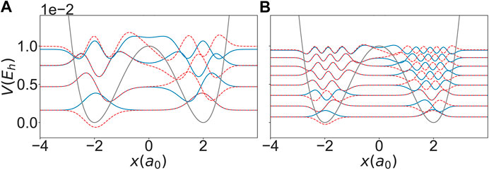
FIGURE 1. Eigenstates for a particle of mass (A)$1m_{\text{H}}$ and (B)$5m_{\text{H}}$ in the potential given by Eq. 21 with $x_{\text{B}}=2a_0$ and $V_{\text{B}}=0.01E_{\text{h}}$. Solid and dashed lines correspond to even and odd eigenstates, respectively.

Using Eqs. 21,22 together with Eq. 7 one can calculate the time-dependent expectation value of the potential, Eq. 12, and its derivatives with respect to α and $x_0$ required for the equations of motion (Eqs. 9, 11). Although in the present case the required expectation value could have been calculated analytically, we have used a more general prescription. To this end the potential is globally approximated by a sum of Gaussians of the form

We have used $g=5$ which gives $g_p=\left\{31.000,-1.529,-1.529,31.000,1.348\right\}$ (in units of $V_{\text{B}}$), $b_p=\left\{1.397,1.658,1.658,1.397,0.\right\}$  (in units of $x_{\text{B}}^{-2}$), and $x_p=\left\{-2.981,-1.142,1.142,2.981,0.\right\}$ (in units of $x_{\text{B}}$).

Using Eq. 23 one obtains for Eq. 12

where

and

For the solution of the control problem the software package PSOPT has been used [40]. This package employs an approximation for the state trajectory of the form

where $t_k$ are the Gauss-Lobatto quadrature nodes $\left(\mathit{a}\left(t_k\right)={\mathit{a}}^N\left(t_k\right)\right)$ and ${\mathrm{ℒ}}_k$ are the Lagrange basis polynomials. This approximation allows to transform the performance functional (Eq. 13) into the performance function

and the differential constraints into a set of holonomic constraints for the decision vector $\mathit{y}=\left(\mathit{u}\left(t_0\right),\dots ,\mathit{u}\left(t_N\right),\mathit{a}\left(t_0\right),\dots ,\mathit{a}\left(t_N\right),\mathit{k},t_0,t_f\right)$; $w_k$ are the Gauss-Lobatto weights. For more details see Ref. [40]. The performance function (30) is optimized using nonlinear programming (NLP) algorithms, such as the ones implemented in IPOPT [41]. PSOPT provides different discretization schemes. The global pseudospectral Legendre and Chebyshev discretization yield very slow convergence for non-smooth functions [19], as it is the case for the solutions found for $\alpha \left(t\right)$ and $\beta \left(t\right)$ (see first and second row, (b) and (d) columns of Figure 2 below). Increasing the number of nodes is not an option for these discretization schemes because of the non-sparsity of the Jacobian matrices which cannot be handled properly by the implemented IPOPT NLP solver. This issue translates into a disproportional increase of computational time. The local methods available are trapezoidal and Hermite-Simpson discretization. In order to check their performance we simulated the case of a particle of mass of $1m_{\text{H}}$ and a final time of $t_{\text{f}}=\mathrm{20,000} \mathrm{a}\mathrm{u}$. In doing so the number of time discretization nodes has been scanned from 200 to 6,000. To evaluate the discretization error we use the maximum relative local error, ${\epsilon }_{\text{disc}}$, defined in Ref. [40]. The results are shown in Figure 3. If the number of nodes is below 1,000 the trapezoidal method has a smaller error ${\epsilon }_{\text{disc}}$ compared to Hermite-Simpson for the same number of nodes. Beyond 1,000 nodes, Hermite-Simpson outperforms the trapezoidal discretization. However, this comes at the expense of an increased computational time as can be seen in the lower panel of Figure 3. For the simulations reported below we have used Hermite-Simpson discretization with 2,000 nodes, which offers a good balance between accuracy and speed.

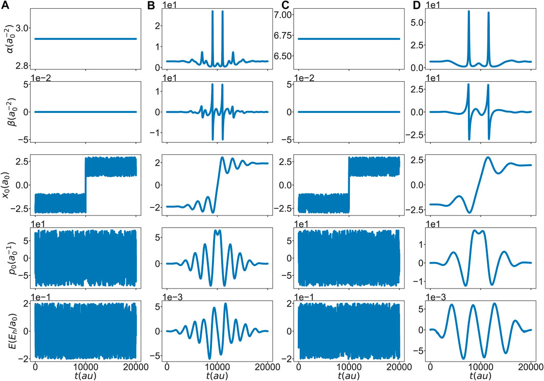
FIGURE 2. Initial guess (A) and (C) and optimal solution (B) and (D) for state, $\mathit{a}(t)$, and control field for two different particle masses ($1m_{\text{H}}$ – (A) and (B), $5m_{\text{H}}$ – (C) and (D)).

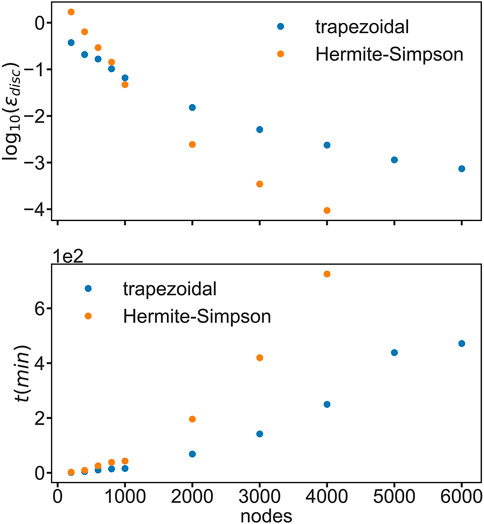
FIGURE 3. Maximum relative local error (upper panel) and timing (lower panel) for trapezoidal (blue) and Hermite-Simpson (orange) as a function of the number of nodes.

In order to quantify the importance of quantum effects beyond the simple Gaussian ansatz for the wavepacket, Eq. 7, MCTDH simulations have been performed using the optimized field. For this purpose the Heidelberg MCTDH package has been used [42].

3 Results

3.1 Laser-Controlled Proton Transfer

In the following we present a proof-of-principle application of direct OCT using the example of proton transfer in a bistable potential. Specifically, the two cases (particle masses) given in Figure 1 will be considered. For the initial state we choose the parameters of a Gaussian in the left well, and as the target state we choose a symmetrically located Gaussian in the right side well. The Gaussian parameters have been optimized to the ground state using a local harmonic approximation. Although direct control in principle allows to vary the final time, in the present application the final time has been fixed to $t_{\text{f}}=\mathrm{20,000} \mathrm{a}\mathrm{u}$. The penalty factor has been chosen as $\kappa =0.3{\mathrm{a}}_0^2/{\mathrm{E}}_{\mathrm{h}}$ (cf. Eq. 18). To solve the problem we also have to provide an initial guess for states and control which is shown in Figures 2A,C. The rapid oscillations have been chosen randomly; there is no correlation between the different variables.

The optimal solutions for the two particle masses are given in Figures 2B,D. Apparently, the optimal field is able to drive the center of the wavepacket across the barrier into the right minimum at $t=t_{\text{f}}$. In this respect one should note that the optimal fields have a relatively simple shape and little resemblance with the initial guess. This is one of the major advantages of the direct approach to optimal control problems, i.e. the convergence region of the initial guess is very broad. The dynamics is rather similar, i.e., in both cases the trajectory passes the barrier coming from the turning point at the left hand side. Just before and after the barrier the wavepacket gets localized in coordinate and delocalized in momentum space, whereas the position-momentum correlation (β) vanishes. The wavepacket passes the top of the barrier with large momentum.

The question now arises if the optimum field found for a single Gaussian wavepacket is able to trigger the same particle dynamics in the full quantum case. To this end the optimal field is used within a quantum dynamics simulation. The results are compared in Figure 4 in terms of coordinate and momentum expectation values and the respective standard deviation. Until after the barrier crossing, Gaussian and full quantum results are rather similar. Indeed, if the goal would have been to trigger the localization of the wavepacket somewhere in the region of the right well at a particular time, the optimal field would still perform this task also in the quantum case. Of course, the agreement between classical and quantum propagation is better in case of the heavier mass even though there is considerable larger spread of the wavepacket in the quantum case after reflection at the right turning point. For the lighter mass the agreement after barrier crossing is less favorable due to the larger spread and the structured character of the quantum wavepacket which cannot be captured by a single Gaussian.

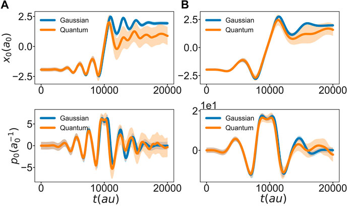
FIGURE 4. Comparison of the coordinate (top row) and momentum (bottom row) expectation values and their respective standard deviation (shaded area), using the Gaussian approximation (blue) and the full quantum propagation (orange). Both trajectories are propagated under the influence of the optimal control field as obtained for the Gaussian (A)$1m_{\text{H}}$(B)$5m_{\text{H}}$).

3.2 Region of Validity of the Gaussian Wavepacket Approximation

Single Gaussians cannot capture the dynamics of structured wavepackets. Nevertheless, the agreement between Gaussian and full quantum results is at least qualitative, even for the lighter particle. This provides the motivation for the investigation of the validity of the Gaussian approximation over a wider range of parameters. Again the optimum field is obtained following the procedure described in Section 3.1, but now for different final times (ranging from $\mathrm{5,000}$ au to $\mathrm{20,000} \mathrm{a}\mathrm{u}$ in steps of $\mathrm{1,000} \mathrm{a}\mathrm{u}$) and masses (ranging from 1 to 10 $m_{\text{H}}$ in steps of 1 $m_{\text{H}}$). To evaluate the performance of the optimum field to drive the wavepacket to the right well in the full quantum case we choose the following error:

where $\tilde{\mathrm{\Psi }}\left(t_f\right)$ is the exact quantum wavefunction at the final time. This error will be between 0 and 1 if the expectation value of the quantum wavepacket crossed the barrier and greater than 1 if it did not. Results are shown in Figure 5.

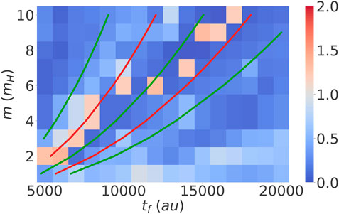
FIGURE 5. Error according to Eq. 31 as a function of different final times and masses. Green lines represent an odd number of half harmonic oscillation periods for the corresponding mass $\left(2n+1\right)T/2$ with $n=\mathrm{1,2,3}$ and red lines represent an integer number of periods $nT$ with $n=\mathrm{2,3}$.

In general, we can see from Figure 5 that the Gaussian optimal control fields are able to drive the particle reaction on a broad range of masses and final times. As expected the performance deteriorates for the lighter masses. There are some features which deserve closer attention. For example, there are regions where the Gaussian wavepacket approach works exceptionally well (characterized by stripes of intense blue color). In these regions the final time is matching a total integer number of well oscillations plus the barrier crossing time. Assuming that these oscillations are harmonic with period T and taking the barrier crossing time as being half of the harmonic period, these final times can be estimated. The middle green line in Figure 5 corresponds to a final time of $5T/2$. It nicely matches with the dark blue region where the approach works well. Thus, in general one would expect regions with $\left(2n+1\right)T/2$ and $nT$ where the approximation works well and not so well, respectively. This is roughly seen in Figure 5, although the deviation from the harmonic approximation causes some quantitative disagreement. This analysis points to the importance of the final time $t_{\text{f}}$ for the effect of the quantumness of the dynamics on the overlap with the target. In passing we note that in principle direct optimal control offers the possibility to optimize the final time as well, e.g., to fulfill some constraints with respect to the spread of the wavepacket.

Another interesting feature apparent from Figure 5 are the isolated “islands” of poor performance, e.g. at $t_f=\mathrm{14,000} \mathrm{a}\mathrm{u}$ and $m=7m_{\text{H}}$. To rationalize this behavior Figure 6 shows various expectation values for $t_f=\mathrm{14,000} \mathrm{a}\mathrm{u}$ and $m=6$ and $7m_{\text{H}}$. The first and second row compares Gaussian and quantum results and we can notice that the corresponding trajectories diverge considerably more for $7m_{\text{H}}$ (b) than for $6m_{\text{H}}$ (a), even though a naive consideration would suggest that the performance of the single Gaussian approximation is better for the more massive particle. In general we observe that while in the good performing cases the wavepacket essentially stays localized, the opposite is true for the poor performing cases, which stands out as a likely reason for the discrepancy between Gaussian and quantum propagation in the later case. This holds irrespective of the actual mass of the particle. From the second and fourth rows of Figure 6 we notice that the cases $m=6$ and $7m_{\text{H}}$ differ in the momentum and thus kinetic energy when crossing the barrier. While in the former case the momentum is maximum at the barrier top, in the latter the particle is slowed down when reaching the barrier. As a consequence it becomes rather delocalized in position space and thus the single Gaussian approximation fails.

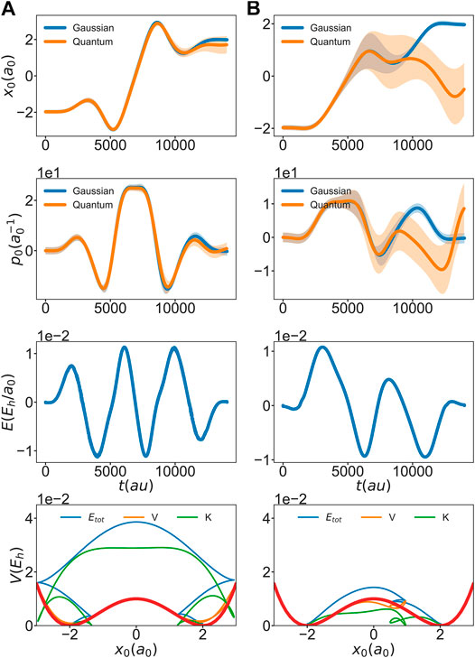
FIGURE 6. Expectation values of coordinate and momentum (shaded areas indicate the standard deviation), optimal field, as well as total ($E_{tot}$), potential (V) and kinetic (K) energy of the moving wave packet (rows from top to bottom) for $t_{\text{f}}=\mathrm{14,000}\mathrm{a}\mathrm{u}$ and (A)$6m_{\text{H}}$, (B)$7m_{\text{H}}$. In the bottom row the expectation values are plotted at the respective positions of the Gaussian wavepacket.

In principle one could expect that decreasing the penalty factor κ would alleviate this problem, i.e. stronger fields would imply higher momentum. However, after inspecting Figure 6, it is apparent that for a given final time it depends on the initial direction of momentum whether the wavepacket will pass the barrier with high or low momentum. This idea supports the conclusion that not only the mass of the particle, but also the specific optimal path, are important for the validity of the single Gaussian approximation. Controlling the initial direction in a way which works in a black-box fashion for all cases covered in Figure 5 has not been successfull. However, in contrast to indirect control, where one would have to compute running cost derivatives with respect to state variables to get coupling terms between forward and backward Schrödinger equation, including additional running costs is straightforward in direct control. To demonstrate this we have added a second term to the running costs of Eq. 18, which serves to maximize the kinetic energy, i.e.

Here, η is a penalty scaling factor and the minus sign ensures that this term gets maximized. It is expected that this will lead to barrier crossing with high momentum and thus a reduced error, Eq. 31.

The results shown in Figure 7 clearly support our hypothesis, i.e. adding the running cost functional Eq. 32 leads to the elimination of the poor-performing islands. Hence, using the flexibility of the direct optimal control approach the region of validity of the single Gaussian approximation could be extended.

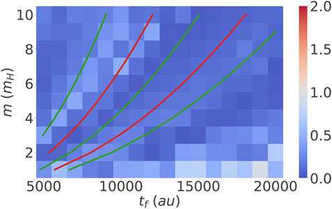
FIGURE 7. Error according to Eq. 31 as a function of different final times and masses. Running cost according to Eq. 32 has been used together with Eq. 18. The penalty scaling factor was $\eta =0.003$, except for a few cases where lower or higher values has been used, ranging from 0.001 to 0.015.

4 Conclusion

In this paper we have introduced a new tool for quantum optimal control. In contrast to indirect methods, which require the solution of a two-point boundary value problem, the present direct method builds on the first discretize and then optimize paradigm. Thus, by construction there is no need for explicit propagation of a wavepacket. So far direct methods have found application mostly in engineering [23, 40]. The performance and capabilities of the direct method have been demonstrated for the case of one-dimensional particle transfer in a bistable potential. For simplicity the wavepacket has been approximated by a single Gaussian function, but in principle other forms are possible, e.g., superposition of Gaussians [28] or even expansions in terms of an eigenstate basis. Of course, Gaussians have the potential advantage of being suited for on-the-fly simulations, which brings OCT into the realm of the dynamics of complex molecular systems, at least in principle. At this point it will be required to explore the scaling of the numerical effort associated with the direct method more thouroughly. Here, we merely explored the dependence on the number of nodes. But the number of parameters will be another limiting factor. Preliminary calculations performed on regular hardware showed that about 50 parameters and 500 nodes are feasible.

For a simple test system the question has been addressed whether the quantumness of the dynamics influences the final control yield, given a field which has been optimized for the single Gaussian approximation. Interestingly, it turned out that nearly complete particle transfer can be achieved for a wide range of masses and final times. Here, the important point is whether the wavepacket crosses the barrier with high or low momentum, which for the given model is decided by the sign of the momentum during the initial dynamics. As a consequence, even the optimization based on a simple Gaussian wavepacket, possibly using on-the-fly dynamics, may provide reasonable control fields.

Data Availability Statement

The raw data supporting the conclusions of this article will be made available by the authors, without undue reservation.

Author Contributions

ARR has performed the work and analyzed the results. OK has designed the project and supervised the scientific work. All authors have discussed and interpreted the results and contributed to writing the article.

Funding

This work has been funded by the grant Ku952/10–1 from the Deutsche Forschungsgemeinschaft (DFG).

Conflict of Interest

The authors declare that the research was conducted in the absence of any commercial or financial relationships that could be construed as a potential conflict of interest.

References

1. Judson RS, Rabitz H. Teaching lasers to control molecules. Phys Rev Lett (1992) 68:1500. doi:10.1103/physrevlett.68.1500
2. Paramonov GK, Savva VA. Resonance effects in molecule vibrational excitation by picosecond laser pulses. Phys Lett A (1983) 97:340–2. doi:10.1016/0375-9601(83)90658-8
3. Tannor DJ, Rice SA. Control of selectivity of chemical reaction via control of wave packet evolution. J Chem Phys (1985) 83:5013–8. doi:10.1063/1.449767
4. Tannor DJ, Kosloff R, Rice SA. Coherent pulse sequence induced control of selectivity of reactions: exact quantum mechanical calculations. J Chem Phys (1986) 85:5805. doi:10.1063/1.451542
5. Brumer P, Shapiro M. Control of unimolecular reactions using coherent light. Chem Phys Lett (1986) 126:541–6. doi:10.1016/s0009-2614(86)80171-3
6. Shi S, Woody A, Rabitz H. Optimal control of selective vibrational excitation in harmonic linear chain molecules. J Chem Phys (1988) 88:6870–83. doi:10.1063/1.454384
7. Shi S, Rabitz H. Selective excitation in harmonic molecular systems by optimally designed fields. Chem Phys (1989) 139:185–99. doi:10.1016/0301-0104(89)90011-6
8. Kosloff R, Rice SA, Gaspard P, Tersigni S, Tannor DJ. Wavepacket dancing: achieving chemical selectivity by shaping light pulses. Chem Phys (1989) 139:201–20. doi:10.1016/0301-0104(89)90012-8
9. Brif C, Chakrabarti R, Rabitz H. Control of quantum phenomena: past, present and future. New J Phys (2010) 12:075008. doi:10.1088/1367-2630/12/7/075008
10. Werschnik J, Gross EKU. Quantum optimal control theory. J Phys B: Mol Opt Phys (2007) 40:R175–211. doi:10.1088/0953-4075/40/18/r01
11. Worth GA, Richings GW. Optimal control by computer. Annu Rep Prog Chem Sect C: Phys Chem (2013) 109:113. doi:10.1039/c3pc90003g
12. Keefer D, de Vivie-Riedle R. Pathways to new applications for quantum control. Acc Chem Res (2018) 51:2279–86. doi:10.1021/acs.accounts.8b00244
13. Brixner T, Gerber G. Quantum control of gas-phase and liquid-phase femtochemistry. ChemPhysChem (2003) 4:418. doi:10.1002/cphc.200200581
14. Prokhorenko VI, Nagy AM, Waschuk SA, Brown LS, Birge RR, Miller RJD. Coherent control of retinal isomerization in bacteriorhodopsin. Science (2006) 313:1257–61. doi:10.1126/science.1130747
15. Stensitzki T, Yang Y, Kozich V, Ahmed AA, Kössl F, Kühn O, et al. Acceleration of a ground-state reaction by selective femtosecond-infrared-laser-pulse excitation. Nat Chem 10 (2018) 126–31. doi:10.1038/nchem.2909
16. Nunes CM, Pereira NAM, Reva I, Amado PSM, Cristiano MLS, Fausto R. Bond-breaking/bond-forming reactions by vibrational excitation: infrared-induced bidirectional tautomerization of matrix-isolated thiotropolone. J Phys Chem Lett (2020) 11:8034–9. doi:10.1021/acs.jpclett.0c02272
17. Heyne K, Kühn O. Infrared laser excitation controlled reaction acceleration in the electronic ground state. J Am Chem Soc (2019) 141:11730–8. doi:10.1021/jacs.9b02600
18. Zhu W, Rabitz H. A rapid monotonically convergent iteration algorithm for quantum optimal control over the expectation value of a positive definite operator. J Chem Phys (1998) 109:385–91. doi:10.1063/1.476575
19. Kelly M. An introduction to trajectory optimization: how to do your own direct collocation. SIAM Rev (2017) 59:849–904. doi:10.1137/16m1062569
20. Kappen HJ. An introduction to stochastic control theory, path integrals and reinforcement learning. AIP Conf Proc (2007) 887:149–81. doi:10.1063/1.2709596
21. Chen-Charpentier BM, Jackson M. Direct and indirect optimal control applied to plant virus propagation with seasonality and delays. J Comput Appl Math (2020) 380:112983. doi:10.1016/j.cam.2020.112983
22. Betts JT. Practical methods for optimal control and estimation using nonlinear programming. Philadelphia, PA: Advances in design and control Society for Industrial and Applied Mathematics (2010).
23. Pardo D, Moller L, Neunert M, Winkler AW, Buchli J. Evaluating direct transcription and nonlinear optimization methods for robot motion planning. IEEE Robot Autom Lett (2016) 1:946–53. doi:10.1109/lra.2016.2527062
24. Meyer H-D, Manthe U, Cederbaum LS. The multi-configurational time-dependent Hartree approach. Chem Phys Lett (1990) 165:73–8. doi:10.1016/0009-2614(90)87014-i
25. Beck M, Jäckle A, Worth GA, Meyer HD. The multiconfiguration time-dependent Hartree (MCTDH) method: a highly efficient algorithm for propagating wavepackets. Phys Rep (2000) 324:1–105. doi:10.1016/s0370-1573(99)00047-2
26. Schröder M, Carreón-Macedo J-L, Brown A. Implementation of an iterative algorithm for optimal control of molecular dynamics into MCTDH. Phys Chem Chem Phys (2008) 10:850. doi:10.1039/b714821f
27. Accardi A, Borowski A, Kühn O. Nonadiabatic quantum dynamics and laser control of Br2in solid argon†. J Phys Chem A (2009) 113:7491–8. doi:10.1021/jp900551n
28. Richings GW, Polyak I, Spinlove KE, Worth GA, Burghardt I, Lasorne B. Quantum dynamics simulations using Gaussian wavepackets: the vMCG method. Int Rev Phys Chem (2015) 34:269–308. doi:10.1080/0144235x.2015.1051354
29. Richings GW, Habershon S. MCTDH on-the-fly: efficient grid-based quantum dynamics without pre-computed potential energy surfaces. J Chem Phys (2018) 148:134116. doi:10.1063/1.5024869
30. Heller EJ. The semiclassical way to dynamics and spectroscopy. Princeton, NJ: Princeton University Press (2018).
31. Kondorskiy A, Nakamura H. Semiclassical formulation of optimal control theory. J Theor Comput Chem (2005) 04:75–87. doi:10.1142/s0219633605001416
32. Kondorskiy A, Mil’nikov G, Nakamura H. Semiclassical guided optimal control of molecular dynamics. Phys Rev A (2005) 72:041401. doi:10.1103/physreva.72.041401
33. Bonačić-Koutecký V, Mitrić R. Theoretical exploration of ultrafast dynamics in atomic clusters: analysis and control. Chem Rev (2005) 105:11–66. doi:10.1021/cr0206925
34. Broeckhove J, Lathouwers L, Kesteloot E, Van Leuven P. On the equivalence of time-dependent variational principles. Chem Phys Lett (1988) 149:547–50. doi:10.1016/0009-2614(88)80380-4
35. Worth GA, Sanz CS. Guiding the time-evolution of a molecule: optical control by computer. Phys Chem Chem Phys (2010) 12:15570. doi:10.1039/c0cp01740j
36. Sundermann K, de Vivie-Riedle R. Extensions to quantum optimal control algorithms and applications to special problems in state selective molecular dynamics. J Chem Phys (2000) 110:1896. doi:10.1063/1.477856
37. Došlić N. Generalization of the Rabi population inversion dynamics in the sub-one-cycle pulse limit. Phys Rev A (2006) 74:013402. doi:10.1103/PhysRevA.74.013402
38. Došlić N, Kühn O, Manz J. Infrared laser pulse controlled ultrafast H-atom switching in two-dimensional asymmetric double well potentials. Ber Bunsen Ges Phys Chem (1998) 102:292–7. doi:10.1002/bbpc.19981020303
39. Došlić N, Abdel-Latif MK, Kühn O. Laser control of single and double proton transfer reactions. Acta Chim Slov (2011) 58:411–24.
40. Becerra VM. Solving complex optimal control problems at no cost with PSOPT. In: IEEE international symposium on computer-aided control system design; 2010 Sept 8–10; Yokohama, Japan. Piscataway, NJ: IEEE (2010). p. 1391–6.
41. Wächter A, Biegler LT. On the implementation of an interior-point filter line-search algorithm for large-scale nonlinear programming. Math Program (2006) 106:25–57. doi:10.1007/s10107-004-0559-y
42. Worth GA, Beck MH, Jäckle A, Meyer HD, Meyer H-D, Vendrell O, et al. The MCTDH package version 8.2 (2000) Version 8.3 (2002) Version 8.4 (2007) Version 8.5 (2011), used Version 8.5.4 Available at: http://mctdh.uni-hd.de/. Tech. rep. (2000).
Keywords: optimal control, quantum dynamics, semiclassical dynamics, Gaussian wavepackets, proton transfer
Citation: Ramos Ramos AR and Kühn O (2021) Direct Optimal Control Approach to Laser-Driven Quantum Particle Dynamics. Front. Phys. 9:615168. doi: 10.3389/fphy.2021.615168
Received: 08 October 2020; Accepted: 09 February 2021;
Published: 23 April 2021.
Edited by:
Tamar Seideman, Northwestern University, United StatesReviewed by:
Ilya Averbukh, Weizmann Institute of Science, IsraelIlia Tutunnikov, Weizmann Institute of Science, Rehovot, Israel, in collaboration with reviewer [IA]
Regina De Vivie-Riedle, Ludwig Maximilian University of Munich, Germany
Copyright © 2021 Ramos Ramos and Kühn. This is an open-access article distributed under the terms of the Creative Commons Attribution License (CC BY). The use, distribution or reproduction in other forums is permitted, provided the original author(s) and the copyright owner(s) are credited and that the original publication in this journal is cited, in accordance with accepted academic practice. No use, distribution or reproduction is permitted which does not comply with these terms.
*Correspondence: O. Kühn, oliver.kuehn@uni-rostock.de