
Automated Residential Energy Audits Using a Smart WiFi Thermostat-Enabled Data Mining Approach


Department of Mechanical and Aerospace Engineering/Renewable and Clean Energy, University of Dayton, Dayton, OH 45469, USA
*
Author to whom correspondence should be addressed.
Energies 2021, 14(9), 2500; https://doi.org/10.3390/en14092500
Submission received: 16 March 2021
/
Revised: 17 April 2021
/
Accepted: 20 April 2021
/
Published: 27 April 2021
(This article belongs to the Special Issue Advances in Energy-Efficient Buildings)
Abstract
:Smart WiFi thermostats, when they first reached the market, were touted as a means for achieving substantial heating and cooling energy cost savings. These savings did not materialize until additional features, such as geofencing, were added. Today, average savings from these thermostats of 10–12% in heating and 15% in cooling for a single-family residence have been reported. This research aims to demonstrate additional potential benefit of these thermostats, namely as a potential instrument for conducting virtual energy audits on residences. In this study, archived smart WiFi thermostat measured temperature data in the form of a power spectrum, corresponding historical weather and energy consumption data, building geometry characteristics, and occupancy data were integrated in order to train a machine learning model to predict attic and wall R-Values, furnace efficiency, and air conditioning seasonal energy efficiency ratio (SEER), all of which were known for all residences in this study. The developed model was validated on residences not used for model development. Validation R-squared values of 0.9408, 0.9421, 0.9536, and 0.9053 for predicting attic and wall R-values, furnace efficiency, and AC SEER, respectively, were realized. This research demonstrates promise for low-cost data-based energy auditing of residences reliant upon smart WiFi thermostats.
1. Introduction
In 2018, according to the U.S. Energy Information Administration (EIA), residential buildings accounted for approximately 21% of total electricity consumption as well as 16% of total natural gas consumption in the U.S. [1,2]. The residential sector has been deemed to offer the most cost-effective potential for energy savings among all U.S. buildings [3]. The most common approach for garnering savings has been through utility rebate programs, whereby utilities offer financial incentives for residential investment in energy reduction measures. The rebated measures are generally those with the statistically best savings relative to investment among the entire residential population. In practice, what this has meant is that all rate payers have effectively subsidized the investments of wealthier residents. Researchers have found that upgrading the housing of low-income residences to the median household efficiency would reduce excess energy by 68%. In other words, while residential energy reduction offers the most cost-effective potential among all U.S. buildings, the vast majority of this savings potential comes from low-income residences [4,5,6].
Many factors impact the energy consumption of individual residential buildings, including weather conditions; building geometry; building thermal envelope materials; heating, ventilation, and air conditioning (HVAC) characteristics; and energy-use behavior of the residents [7,8]. However, identifying the energy efficiency priorities for individual residences is not automatic and can be both laborious and expensive. For example, traditional energy audits require a physical visit to a residence, whereby a technician performs air leakage tests; conducts infrared imaging; documents insulation in the walls, basement/crawlspace/sub-flooring, and attic; and assesses the efficiency of the heating/cooling/water heating systems. These audits can be costly [9]. The U.S. Department of Energy estimates costs for detailed energy audits ranging from $0.12 up to $0.503 per square foot, depending on the size and complexity of the residential buildings [10]. In another study, the average cost to audit single-family residences in the US starts at $400 and increases dramatically with the size of the home [11]. The audit cost can outweigh the potential energy cost savings, and the recommendations made have been observed to be dependent on the auditor [9,12]. For example, a study compared recommendations from three different contractors hired to audit the energy effectiveness of three different types of buildings: namely a large multi-family residence with a common heating plant, a primary school, and a terraced or row home. The final recommendations from the three different contractors were quite dependent on the auditors, with installation cost and savings estimations respectively differing by as much as 300% and 250% relative to the lowest estimates [13]. Likewise, another study compared three energy audit reports conducted on the same building [12]. The three studies reported widely divergent results. First, the three reports employed different audit data. Second, the list of energy conservation measures (ECMs), short of three common measures, were different. Third, the initial cost and energy and cost savings for the shared ECMs varied widely between the analyses. Additionally, the energy audits cost from three different companies ranged from $252 to $1123. This trend has certainly contributed to a lack of faith about the value of residential energy audits [9,14]. Importantly, low- to low–middle-income residents frankly will never opt to have their residence audited. The expense just cannot be tolerated.
There is a strong need for automatically auditing the energy effectiveness of residences at a substantially lower cost. Such audit-derived information could help to change the paradigm for utility rebate programs were every residence within a utility district to be audited. A ‘worst-to-first’ priority for utility investment in energy reduction could be established in such a way as to ensure that the investments made yield the biggest energy and energy cost savings [15,16].
Recently, smart WiFi thermostat adoption in the U.S. market has seen rapid growth. An ACEEE study estimated that by 2020, over 40% of residences would have this technology in it [17]. The data from these thermostats is especially valuable in documenting heating, cooling, and ventilation energy consumption. For example, Hossain et al. [18] utilized smart thermostat data to develop dynamic thermal models of residences. Additionally, Huang et al. [19] utilized smart WiFi thermostat data to predict room temperature and cooling/heating demand, as well as potential savings from changes in thermostat settings. Another study by Stopps et al. [20] used data from 54 smart thermostats to analyze programming and occupant interaction behaviors. Likewise, Lou et al. [21] employed a smart WiFi thermostat to calculate temperature and humidity setpoints that would meet the minimum thermal comfort at all times. This latter study showed cooling energy savings in excess of 70% from thermal comfort control.
2. Background
In this section, relevant research pertaining to the standard calculation approaches is presented for: building energy models with sufficient granularity to permit estimates of savings from residential energy upgrades, inverse modeling approaches with sufficient granularity to identify residences in need of upgrades and quantity the resulting savings based on energy data pre- and post-upgrade, and the state-of-the art associated with virtual energy audits.
2.1. Building Information Modeling and Simulation for Energy Audits
Energy modeling software (e.g., eQuest, EnergyPlus, IES, and Energy-10) has been used extensively to simulate and predict building energy consumption. Generally, these have required extensive detail about the geometric and energy characteristics of a building, as well as occupancy and control schedules. Examples of their use are extensive and, unfortunately, despite the detail required of data inputs, the energy savings recommendations that result have been very inconsistent [22]. For example, one study evaluated the accuracy of the United States Department of Energy (DOE)-developed eQuest software for predicting energy consumption and estimating savings from upgrades in hotels. Good correspondence was seen between predicted and actual savings based on the building energy efficiency retrofit (BEER) scheme [23]. However, other studies have demonstrated just the opposite [24]. These tools are strongly dependent on the user and require significant engineering time [25]. Much of the time, these tools overpredict energy consumption [16]. For example, the Energy Trust of Oregon performed a study to evaluate building energy simulation programs. Three programs were compared: SIMPLE, REM/Rate, and Home Energy Saver (HES). Detailed audits were conducted, and utility bills were collected for 190 homes. The homes were simulated with the three energy modeling tools, including two levels of detail for HES. The models overpredicted gas use for space heating by an average of 41% in older homes built before 1960 and by 13% for newer homes built after 1989 [26,27]. Likewise, the validity of the Manufactured Home Energy Audit tool was assessed in a two-part study by Oak Ridge National Laboratory (ORNL). Obtained audit and utility data were used to analyze the energy effectiveness of manufactured homes across five counties in the U.S. North and Midwest. The predicted space heating energy consumption was compared to the actual space heating energy consumption. Pre- and post-retrofit comparisons of modeled and actual energy use were made. Results from the pre-retrofit simulations were observed to overpredict space heating energy use from 163% to 109% [28]. Lastly, a recent study by Pacific Northwest National Laboratory on seven homes with deep retrofits showed a range of predicted savings obtained by different auditors from 75% overestimation to 16% underestimation relative to the savings realized for all the homes evaluated [29].
2.2. Inverse Energy Modeling for Identifying Residences in Need of Upgrade and Estimating Savings from Upgrades
In 1994, ASHRAE published an Inverse Modeling Toolkit (IMT), which has been used since to estimate savings from various system upgrades [30]. This toolkit is based on a four-step process. The first step is to create statistical three-parameter models of electricity and natural gas consumption as a function of the outdoor air temperature over the energy consumption period. This regression renders estimates of the sensitivity of the consumption to temperature (termed heating and cooling slopes), the building balance-point temperature, and average weather-dependent energy consumption for a meter period. The second step is to apply these to site-relevant typical meteorological year (TMY3) weather data to determine the normalized annual consumption (NAC) for each type of energy. The third step is to derive an NAC for each set of 12 sequential months of utility data. The fourth step is to compare the NACs of multiple buildings to identify average, best, and worst energy performers and to evaluate how the consumption of a building has changed over time. It is this last step that permits measurement of savings post-retrofit of energy efficiency upgrades [31].
A case study of 14 Midwest hospital results showed that the NAC analysis is more stable and informative than the regression coefficients determined from the first step. Additionally, a change in NAC indicates a real change in the energy performance of the building, provided that the savings are greater than 10% (note that ASHRAE suggests that this approach is not, in general, able to measure savings less than 10% [16]). In another study, electric and natural gas historical consumption data were merged with residential building geometry, and historical weather data to determine the energy consumption intensity for each home in a Village of Yellow Springs, Ohio by using a five-parameter fit for the electricity data and a three-parameter fit for the natural gas data. These researchers normalized the NAC calculations with the residential floor area. Using this normalized data, they were able to identify the most promising homes for energy reduction [32].
2.3. State-Of-The-Art in Virtual Energy Audits
Building geometric and energy characteristics (insulation type and amount in envelope components, heating/cooling/water heating efficiencies, etc.) have a prominent influence on energy consumption [33]. Knowledge of these characteristics is essential for estimating potential energy savings from specific energy upgrades. Ordinarily, such data is collected from on-site audits. However, there have been some recent strides toward inferring energy characteristics from data alone. Table 1 summarizes research to predict the energy characteristics of buildings or to disaggregate the energy consumption into specific categories, such as lighting and appliances.
The private company Retroficiency (acquired by ENGIE Insight) claimed in the mid-2010s to have the ability to automatically audit the energy performance of commercial buildings. Their approach employed interval energy data from smart meters, occupant schedules, weather, and systems control details. Their virtual energy assessment (VEA) provided recommendations for retrofits based upon the virtual audit. Included in their recommendation were estimates of upgrade costs and return on investment [34].
In 2016, Case Western Reserve University and Johnson Controls Inc. worked collaboratively to develop another version of a virtual energy audit for small- to medium-sized commercial or retail buildings. Their approach employed 15-min-interval utility data, insulation characteristics, and weather data [35]. Lastly, the approaches by FirstFuel, Agilis Energy, and C3 Commercial likewise employ interval meter data from smart meters and real-time weather data to estimate various forms of electric consumption (lighting, cooling, etc.).

Table 1.
Summary of prior research in predicting energy characteristics in buildings.
| Ref. | Software/Company Name | Learning Algorithm (Type) | Types of Feature | Building Type | Target |
|---|---|---|---|---|---|
| [34,36] | Retroficiency, Retroficiency, USA | Proprietary algorithm (Not for public use) | Smart meters, occupant behavior, weather, and systems control details | commercial | Heating, cooling, ventilation, lighting, plug loads, pumps, domestic hot water systems |
| [35,37] | Case Western Reserve University, Great Lakes Energy Institute (GLEI) | Energy Diagnostics Investigator for Efficiency Savings (EDIFES) (Not for public use) | Smart utility meter, insulation information, operation schedules, weather data | commercial | Exterior lighting (e.g., 24-h lighting and security/monitoring systems), HVAC (e.g., heating, ventilation, and air conditioning electricity consumption), and occupancy-based plug loads (e.g., computers, refrigerators, copiers, televisions, interior lighting, etc.) |
| [34,36] | FirstFuel, Tendril, USA | Statistical model (Not for public use) | Hourly electricity consumption data, hourly local weather data, high level building data from geographic information systems | commercial | Electric lighting, building envelope, equipment, HVAC, service hot water, operating schedule |
| [34,36] | Agilis Energy, Agilis, USA | Statistical model (Not for public use) | Smart meter interval data and climate data | commercial | Operational energy performance, interval energy demand, occupancy, energy system operations |
| [34,36] | C3 Commercial, C3 Energy, USA | Statistical model, Database for Energy Efficiency Resources (DEER) (Not for public use) | Smart meters data drives inverse modeling and uses national, state, and regional utility building stock data for benchmarks to compare energy benchmark with other buildings that are functionally equivalent (same type and floor area) | commercial | Electric lighting, building envelope, equipment, HVAC, service hot water, and operating schedule based on data driven inverse energy modeling, coupled with statistical analysis utilizing an existing energy conservation measures (ECM) list from the database for energy efficiency resources (DEER) |
3. Objectives of Research
While smart meters have gained an increasing market share [38], nationally, there is still no consistent standard relative to the frequency of data collection and input [39]. Their use in this study is not assumed. For many residences, only monthly interval energy consumption data is available. Moreover, smart meters are only generally capable of providing information about electricity consumption. The cost for smart gas meters is prohibitive for wide-scale use without some type of enabling subsidy.
There are three starting points for this research. First, a smart thermostat offers greater promise for characterizing heating-, cooling-, and ventilation-related energy characteristics than smart meters, which are more prevalent in both the U.S. and Europe because smart WiFi thermostats provide for measurement of the internal residence temperature and humidity and account for residence-specific controls on this temperature. Second, the monthly metered energy consumption reflects the overall heating and cooling energy effectiveness of a residence. However, this information alone is incapable of resolving specific contributions to the heating and cooling energy effectiveness. Third, it acknowledges that if the residential energy characteristics for a sub-set of residences are known, data-based machine learning based models can be tuned to predict the individual energy characteristics. If these models are derived from data collected from numerous diverse residences, theoretically, they could then be used to predict the energy characteristics in residences where these are unknown.
The research question driving this study is the following: “How can the individual contributions to the heating and cooling energy effectiveness (namely the envelope R-values and heating/cooling system efficiencies) be resolved from only remotely collected data? To date, this question has not been answered.
Fundamentally, the goal of this research is to estimate residential energy characteristics from monthly energy consumption (potentially gas and electric), coupled with other data that could be collected remotely for residences. This data includes historical weather data, residential building geometry data, and potentially occupancy data, and uniquely and most importantly, smart WiFi thermostat data. This latter data, because of the relative high frequency associated with its measurement, could potentially help to resolve the energy characteristics, which control the thermal dynamics of a residence to heat gain/loss to changes in outdoor weather and to internal heating and cooling. If it was possible for these instruments to make possible remote energy auditing of residences, their prevalence in the world would guarantee wide-scale impact. In 2017, more than 82 million smart thermostats were in use in North America according to a study by Berg Insight. The same study projected that more than half (51%) of North America homes would be smart homes by 2022 [40].
To achieve the broad goal of predicting residential envelope R-values and heating/cooling system efficiencies from the varied data types (static residence geometrical, occupancy, and energy characteristics; monthly metered energy consumption; higher frequency weather data; and high-frequency ‘delta’ smart WiFi thermostat data), it is necessary to extract useable features from the higher frequency signals in order to combine with the monthly metered consumption. This first requires the creation of derived features characterizing the weather variation within the energy consumption meter periods. Average outdoor temperature during a meter period is not sufficient to characterize the exterior weather. Secondly, it requires the development of dynamic characteristics based upon smart WiFi thermostat data unique to a residence in which a smart WiFi thermostat is present. With static representations of the dynamics of the outdoor weather for each meter period and a residence’s response to dynamic changes established, the data could be combined and then used to train machine learning models on a sub-set of residences for which the energy characteristics are known. Last, the developed model must be tested on residences not used in the training to demonstrate the potential for this approach to estimate energy characteristics in residences where the energy characteristics are unknown.
This paper is organized as follows. First, as the approach posed hinges on the data used, the data employed in this study are described. Next, the methodology and results, both aligned with the objectives posed, are presented. Lastly, we conclude by discussing the wide-scale implications of the approach developed to remote regional energy auditing and the work that is required to realize this potential.
4. Data
There were four main raw data used in this study. A description and more details for each individual dataset are contained in the following subsections.
4.1. Residence Geometrical, Occupancy, Monthly Energy Consumption, Energy Characteristics, and Smart WiFi Thermostat Data
This study considered 101 houses owned by a university in the Midwest region of the U.S. The majority of these houses are detached single-family houses constructed of wooden materials (with low thermal mass). Geometrical data were accessed for all residences through the local county property database. Such data is publicly available nationally.
Second, historical monthly energy consumption and occupancy data (electric and gas meter data) from January 2016 to the present were obtained for each residence from the university owner of the residences.
Third, energy characteristics for these residences were acquired in 2015 through detailed energy audits made by one of the lead authors. As noted in a prior study, this audited subset of houses offered significant diversity in size, insulation, and energy effectiveness as shown in [16], which helps in developing a generalizable model capable of predicting energy characteristics in any residence.
Table 2 shows the minimum and maximum values for the building geometric data, energy characteristics, and residential occupancy characteristics for the 101 residences considered. Some input features included in the table might in general be a challenge to acquire (e.g., refrigerator-related data) but are retained here in order to evaluate their importance.
Smart WiFi thermostats data were accessible for each of the audited residences. Raw thermostat data, referred to as “delta data”, were collected for each of the residences. Delta data are logged only when there is a change in one of the thermostat features. In practice, this means that if the set point temperature, measured temperature and humidity at the thermostat, heating/cooling mode, or heating/cooling/fan status changes, data are recorded. For this research, smart WiFi thermostat data for these houses were continuously collected and archived from 6/1/2018 to the present. Typically, thousands of points were collected for each residence each month.
There is only a single smart WiFi thermostat (one point) in each house. The houses were intermittently heated/cooled throughout the day based on the thermostat setpoint temperature. Additionally, all house thermostats were monitored by the university housing management to ensure they were within the reasonable setpoint temperature range. Moreover, the residents were strongly advised to keep the windows closed when their residence was employing air conditioning.
4.2. Weather Data
5. Methodology
The methodology is organized as follows. In the first two sub-sections, the process for extracting features characterizing respectively the variation of the weather data in each meter period and the thermal dynamics of each residence to changes in outdoor temperature and internal heating and cooling as evidenced from the smart WiFi thermostat data is described. Then, the data-based machine learning and testing approaches are described.
5.1. Development of New Weather Features Characterizing Outdoor Temperature Variation during Each Meter Period
Inverse energy models have employed mean outdoor average temperature for an entire meter period as an input (often singular) to predict energy consumption [31]. However, including increased granularity to better reflect variation that occurs over a large time period may be beneficial.
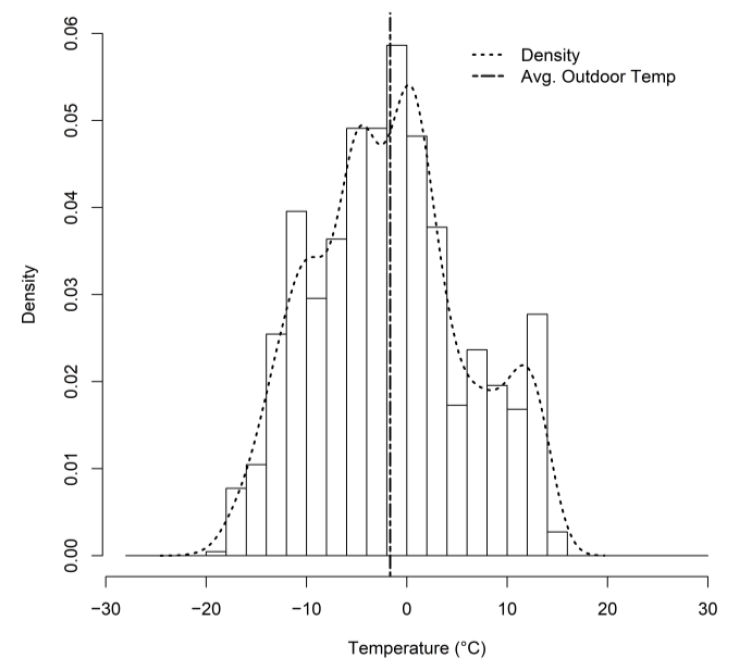
The approach used here is to ‘bin’ the outdoor temperature data within a meter period into discrete temperature bands, determining the probability density of the outdoor temperature in each of the discrete bands over one energy consumption meter period. The idea is that it is not just the mean temperature in a meter period that is important. Rather, the record of temperature variation in a meter period is even more important, especially if the thermostat set point temperature is changing within the meter period.
5.2. Development of Dynamic Representations of Smart WiFi Thermostat Data for Each Residence
The measured smart WiFi thermostat temperature provides a record of heat gain/loss from the residence from/to the outdoor environment and a record of heating and cooling. When the heating system and cooling system are on, the interior temperature is observed to warm/cool over a certain amount of time. So, in effect, it accounts for the time constants associated with the heating and cooling systems, which likewise depend upon the heating and cooling system efficiencies. After heating and cooling is interrupted, heat loss/gain to/from the outdoor environment is registered as a decrease/increase in internal temperature. The rate at which the internal temperature cools/warms after interruption of heating/cools depends upon the envelope heat losses/gain, and thus on the thermal capacitances (time constants) associated with the envelope components and infiltration.
Since the aim of this research is to develop single models to predict residential energy characteristics based upon data from numerous diverse residences, we looked to develop a representation of the measured smart WiFi thermostat that could potentially account for the different time constants associated with the envelope barriers and the heating/cooling systems. A power spectrum reduction of this measured temperature seemed a reasonable approach; as such, a representation characterizes the strength of a signal relative to the driving frequencies.
In order to develop a power spectrum on a signal, however, the signal frequency must be constant. This was not the case for the smart WiFi thermostat data measured here [43]. “Delta” thermostat data is non-uniformly spaced in time. So, step 1 in establishing power spectrum representations of the measured smart WiFi thermostat temperature was to create a uniformly spaced signal. Linear interpolation was employed to estimate the temperature at fixed intervals based upon the measured thermostat temperatures, using Equation (1):
where a, b, and in this case are times associated with the collected data; and are collected neighbor data points at and (); and is interpolated data.
The characteristic frequency of each residence to changes in outdoor weather conditions is an indicator of the dynamic thermal characteristics of a residence’s envelope elements (walls, windows, and ceiling). The power spectrum defines the ‘strength’ of the response (measured thermostat temperature) with frequency. The power spectral density h(ω) is equal to the correlation value γ(k) (where k is lag and t is time) divided by the frequency span over which that peak is observed e-iωt (Equations (2) and (3)) [44]:
A locally high amplitude in the power spectrum at a specific frequency means that the measured signal (thermostat temperature) owes much of its energy to a dynamic phenomenon at this frequency. For example, higher efficiency houses have more energy in the signal at lower frequencies, so if something changes outside or the set point temperature changes inside, the response to change as measured by the thermostat temperature is slow. In the power spectrum, the peak is in the low-frequency band. On the other hand, lower efficiency houses have more energy at higher frequencies.
In this study, a histogram of the power spectra for each house was created for fixed period bands. A total of 500 uniformly spaced bins were set. The average signal strength in each bin was calculated. Thus, the available power spectrum binned data was available for each residence. Of these, only the first 50 bins were retained, corresponding to 48-h periods. Table A1 shows the range of values for each bin in the first 50 bins retained. Almost all of the signal energy for each residence resided in these bands. In effect, this binned power spectra data is a characteristic of a residence. It should be noted that the thermostat data period used was in the middle of the summer/winter season. In the summer, most of these residences were non-occupied (yet still air conditioned) to prevent mold formation. Thus, windows were almost always closed. In the winter, few if any windows were opened by residents.
5.3. Development of Data-Based Machine Learning Models for Each Envelope Thermal Resistances and Heating/Cooling System Efficiency
5.3.1. Data Merging and Preparation
In order to develop machine learning models for predicting the individual energy characteristics from the data described in Section 4 and developed in Section 5.1 and Section 5.2, the data was merged. The binned outdoor temperature for each meter period and the binned smart WiFi thermostat temperature power spectra, along with the static residential geometry, occupancy, and energy characteristics, were synched and merged with the monthly energy consumption data by common address.
Additionally, in order to mitigate observation bias, very similar houses were removed by measure distances between the houses. A K-means Euclidean distance [45] was computed from the standardized static residential data only. The analysis found 14 similar houses (including 3 very similar newer houses). As a result, 9 houses were eliminated from inclusion in the model training datasets. As a result, the total number of residences included in the training dataset was reduced to be 86 houses. Then, all observations with any missing data were eliminated [46].
5.3.2. Model Development and Testing
Choosing the right machine learning algorithm is complicated; it depends on the data type, number of observations, number of input features, etc. Additionally, the second major challenge is to tune the model hyperparameters. Different machine learning algorithms have different hyperparameters, which need to be optimized in order to yield the best models. For example, the most critical hyperparameters in artificial neural network (ANN) models are the number of hidden layers, dropout rate, network weight initialization, activation function, learning rate, momentum, number of epochs, batch size, etc. [47,48]. In this research, the AutoMLH2O package [49] was used to select and tune the model and hyperparameters. Functional forms considered in this approach included deep neural networks, random forests, extremely randomized trees, gradient boosting machines (GBMs), extreme gradient boosting (XGBoost), and stacked ensembles. Table 3 shows the input features employed to predict the attic R-value, wall R-value, furnace efficiency, and AC SEER targets. Note the R-value targets use as input features knowledge of the furnace efficiency and AC SEER, but the latter two do not leverage the attic and wall R-Values as features. Thus, the general predictive process would be to first predict the R-values and then use these predictions as predictors for the furnace efficiency and AC SEER.
A training dataset was used to develop a predictive model, while a validation dataset provided an evaluation of the model for model hyperparameter tuning. Next, the model was applied to an independent testing dataset. We used 10-fold cross-validation during hyperparameter tuning to avoid subset biases. We reported and used the mean cross-validation performance metrics [50,51,52].
The effectiveness of the models for both the validation and testing datasets was evaluated using the following parameters: R-squared metric, mean square error (MSE), root mean squared error (RMSE), mean absolute error (MAE), and root mean squared logarithmic error (RMSLE):
A model is only as good as its ability to make accurate predictions on data not used in its training. Here, the true quality of the models developed was assessed through testing. A testing dataset was developed by extracting the observations from 6 houses from among the 92 houses included in the study. The six testing houses were randomly selected but were also checked to ensure that the testing set included high, medium, and low values of the responses (Table 4).
6. Results
6.1. Development of New Weather Features Characterizing Outdoor Temperature Variation during Each Meter Period
Figure 1 shows a representative probability density distribution for the outdoor temperature developed for a single meter period within discrete two degree °C bins. This figure shows how this binning took place for one meter period (1 January 2018 to 9 February 2018).
6.2. Development of Dynamic Representations of Smart WiFi Thermostat Data for Each Residence
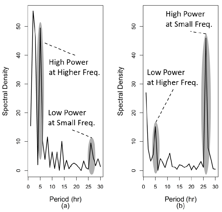
Figure 2a shows the power spectrum for an energy-effective residence with respective wall and ceiling R-values of 2.46 and 3.16 (m2 × K × W−1), whereas Figure 2b shows the power spectrum for a low-energy-effective residence with respective wall and ceiling R-values of 0.70 and 2.28 (m2 × K × W−1). Note that in the former case (a), most of the energy in the signal is at small periods, the opposite of that for the low-energy-effectiveness case, owing to the more rapid response of high-efficiency homes to heating and cooling, relative to a slower, more damped response (due to greater heat loss/gain to the external ambient) for the low-efficiency residence. Most visible is that at the diurnal period (24 h), there is little energy in the high-efficiency house case, but, in comparison, the signal energy peaks at this period for the low-efficiency house case. Thus, the low-efficiency house ‘feels’ the diurnal transients far more than the high-efficiency house, which damps out most of the energy associated with this cycle.
The higher energy at lower periods (higher frequencies) for the high-efficiency residence in comparison to a low-efficiency residence is primarily affected by the response to thermostat set point changes. The high-efficiency house is able to respond quickly to indoor temperature set point changes. The low-efficiency house responds more slowly. So, even the period associated with set point changes increases relative to the high-efficiency house case.
6.3. Training and Testing of Data-Based Machine Learning Models for Each Envelope Thermal Resistances and Heating/Cooling System Efficiency
6.3.1. Identifying the Best Machine Learning Algorithm
This subsection aims to document how the best model was developed in predicting each of the envelope thermal characteristics. It was unknown what model algorithm should be used and which features should be included in the model development.
First, different machine learning algorithms were applied and validated on the complete training dataset. This complete dataset included all static residential features, monthly energy consumption, binned outdoor temperature data for each meter period, and all binned smart WiFi thermostat temperature power spectrum data.
Table 5 documents the validation metrics obtained for this complete dataset for the various algorithms employed. It is clear from this table that the GBM machine learning methodology yielded the best validation performance. Hereafter, only this algorithm was considered. The general formula for gradient boosting machine (GBM) is shown in Equation (9), which can be applied to all four targets [53]:
where bτm(x) ∈ β is a weak learner and βm is its corresponding additive coefficient.
6.3.2. Identifying the Best Thermostat-Derived Feature Set for Model Development
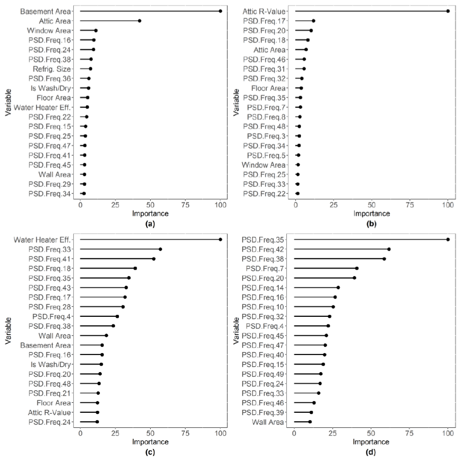
Figure 3 shows variable importance plots obtained from the best GBM models produced in predicting the (a) attic R-value, (b) wall R-value, (c) furnace efficiency, and (d) AC SEER. In this figure, the features labeled PSD.Freq.X refer to the average power spectrum powers in frequency bin X. It is clear from this figure that the power spectrum features are very important for predicting each of the energy characteristics. As a result, one would expect that the spectral information present in the thermostat signals improves the prediction of the targeted energy characteristics.
We then investigated developing models using subsets of the PSD.Freq.X data. GBM models were thus developed to predict the targeted energy characteristics for the following PSD binned power subsets: (a) for the first 40 frequency bins (approximately needed to capture the diurnal cycle), (b) for the first 20 frequency bins, (c) for the first 10 frequency bins, (d) for the top 10 most important frequency bins for each target obtained from a variable importance analysis using the best GBM model, (e) for the top 2 frequency bins for each target obtained from a variable importance analysis, (f) for the top frequency bin for each target for each target obtained from a variable importance analysis, (g) for the top two frequency bins for each target obtained from an optimization to minimize error, and (h) for the top frequency bin for each target obtained from an optimization to minimize error.
Table 6 shows the testing statistics for predicting the attic and wall R-values, furnace efficiency, and AC SEER, respectively, for inclusion of the binned spectral powers using the same testing dataset considered in Section 5.3.2. There are three main points to make. First, while some of these cases yield accurate validation metrics for individual targets, the best overall cases are those using only one or two of the optimally selected frequency bins to minimize the validation error. It is clear that the use of all of the frequency bins introduces many features that have little influence on the target. Elimination of these features in general improves the model. Second, the prediction statistics for the testing dataset are improved markedly for the last three cases, cases e–h. Case e, where the two top power spectrum bins were based upon the GBM variable importance, yielded the best model for predicting the attic R-value. Case g, which included as predictors the two most important power spectrum frequency bins for minimizing error, yielded the best model for the AC SEER. Lastly, case h, reliant upon a single power spectrum frequency bin based upon minimizing the predictive error, yielded the best model for predicting the wall R-value and furnace efficiency. The best MAE error in predicting the attic R-value, wall R-value, furnace efficiency, and AC SEER was reduced from 0.5249 to 0.2752, 0.2768 to 0.1044, 0.0362 to 0.0116, and 0.7450 to 0.4245, respectively. All of these errors could be well-tolerated in virtual energy audits.
It is interesting in this table to see how the use of multiple power spectrum frequencies especially harms the models in predicting the AC SEER and furnace efficiencies (cases a–d). The fact is that the ac and furnace systems for the set of residences are respectively two- and single-stage systems, meaning that the cooling and heating powers respectively have two and one levels. Having multiple power spectrum frequency bins to predict the cooling/heating system efficiencies is seen to actually hurt the performance of the regression. Additionally, it is interesting to see the progressive improvement in model accuracy for predicting all of the features as a result of using a reduced number of power spectrum frequencies obtained either from the variable importance characterization from the GBM model or through error minimization. This in effect says that the different features are associated with specific frequencies. For example, the best model in predicting the furnace efficiency is associated with a single binned power spectrum efficiency of 46. Given that only the single-stage furnaces are considered in this study, all with constant heating power, the time response associated with furnace on-time dictates that a single frequency should best characterize this system. In comparison, a majority of the AC systems considered in this study had two stages associated with different cooling powers. Thus, it is not surprising that two power spectrum bins capture the dynamics of these systems best. Similarly, the attic and wall R-values control the dynamics associated with cooling of the internal environment. Again, a single frequency should best characterize the dynamics of these components.
Table 7 summarizes the best model testing performance for each of the targeted energy characteristics obtained from Table 6. Table 8 shows the actual values and predicted values of these characteristics using these best models for all of the testing houses. Model performance appears strong across evaluation metrics. The errors associated with the prediction of each energy are quite small for all of the residences. These errors could well be tolerated in any energy audit.
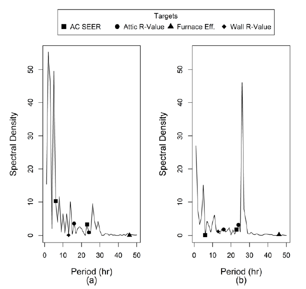
Figure 4 helps to illustrate the most important power spectrum density (PSD) frequency for each target, and how each frequency is different from a high- and low-efficiency house. First, the following dominant PSD frequencies: 6, 16, 23, and 46, show high power in high-efficiency houses and low power in low-efficiency houses. Second, the dominant PSD frequencies, 13 and 24, show low power in high-efficiency houses and high power in low-efficiency houses.
6.3.3. Summary of the Best Model Validation Statistics and Hyperparameters
6.3.4. Identifying the Value of the Thermostat-Derived Features for Predicting Energy Characteristics
Table 11 summarizes the validation metrics for predicting the targeted attic R-value, wall R-value, natural gas furnace efficiency, and air conditioner SEER value for the various models considered using the complete training data features, e.g., considering the case where thermostat-derived power spectrum binned data is not included. From this table, it is clear that it yielded strikingly good model results, with respective R-squared values of 1, 1, 1, and 0.99 and RMSE errors of 0.0022, 0.0013, 0.0002, and 0.1513 for predicting the attic R-value, wall R-value, furnace efficiency, and AC SEER. The tuned hyperparameters (number of trees, number of internal trees, depth, and minimum number of observations in the smallest leaf) for the best GBM models are shown in Table 12.
The hyperparameters of the best model without using thermostat-derived information shown in Table 12 are compared to the hyperparameters of the best model obtained using thermostat-derived information shown in Table 10. It should be noted that the number of trees and the minimum number of observations in the minimum leaf are within the recommended values, which are 2/3 the number of observations and 12 observations per leaf, respectively. Furthermore, there is similarity in all of the hyperparameters, providing an indication of the confidence that the models developed to predict the energy characteristics using thermostat-derived data is not simply overfitted relative to the case where thermostat data were excluded.
The developed models were then applied to the testing set of houses described previously. Table 13 shows the actual values and predicted values of the targeted energy characteristics. The models were generally accurate in predicting the energy characteristics; however, the AC SEER values in the training data set did not have as much variation as desired, thus the predictions of these had the greatest associated error. The testing results were as follows (see Table 14). The R-squared and MAE values for predicting the attic R-value, wall R-value, furnace efficiency, and AC SEER were respectively 0.6778, 0.6474, 0.6280, and 0.5928 (R-squared), and 0.5249, 0.2768, 0.0362, and 0.7450 (MAE). These results are significantly poorer than the predictions reliant upon the thermostat-derived information.
7. Conclusions and Discussion
This study has demonstrated the feasibility of utilizing available residential building data, historical energy consumption, and archived smart WiFi thermostat data to develop machine learning models to predict with accuracy the primary heating and cooling characteristics of a residence provided there is a set of residences for which the energy characteristics have been measured for. Residences with known energy characteristics, if they reflect the whole pool of residences in a particular area, can be used to effectively calibrate a data-based model, which can then be used to predict energy characteristics in other residences. Uniquely, this research has shown the value of thermostat-derived data characterizing the dynamic response of residential inside temperature to weather and thermostat set point changes in improving the accuracy of these predictions.
The potential implication of this research is substantial. The data needed to render this information is potentially accessible. Generally, smart WiFi thermostat data is accessed via the cloud by the thermostat manufacturer. This research is premised on the idea that such companies could directly manage or indirectly participate in a regional electric and/or gas utility sponsored program to audit residences leveraging smart WiFi thermostats. Through such an arrangement, the smart WiFi thermostat manager would also have access to metered energy consumption for all participating residences. If data for all types of possible residences could be collected, at least within the boundaries of a utility service territory, a single model could be trained to predict the most important energy characteristics that would be applicable to every residence in a region. Potential savings from upgrades of every energy characteristic in each residence could be estimated. A strategic energy (and carbon) reduction investment protocol could be established to realize the greatest savings per investment, and in a way that did not exclude low- to low–middle-income residences.
Admittedly, there is more work to do. One, the dataset used for training must be expanded. All of the houses considered in this study were two-story wood-frame houses. Data from brick, stone, single-story, duplex, etc. residences must be added to the growing database of residences to expand the relevance of this research to the whole of the U.S. and the rest of the developed world, where buildings generally have much higher thermal mass. It is certain that the approach posed here could be likewise used in such buildings; however, new predictive features characterizing the construction type (brick, stone, etc.) would be needed to generalize the model developed. Additionally, other features characterizing the placement of a residence relative to adjacent residences, such as single-family detached, condo, apartment, etc., could be added as predictors.
Further, there is an opportunity to combine data derived from smart WiFi thermostats and smart interval meters to expand the information derived. In the U.S., nearly 70% of residences are equipped with smart meters [54]. In Europe, the adoption of this technology is even more pervasive [55]. If both datasets were to be leveraged, the source power for cooling, heating (if heat pump), and ventilation could be determined. Energy savings estimations from upgrades of the HVAC energy savings retrofits could as a result be more accurately calculated.
In addition, this study only used one thermostat-derived piece of information. The thermostat temperature set point history could and should also be considered. Finally, solar fenestration has a clear impact on the dynamics of residences, especially those with large window areas. Future research should include solar irradiation dynamic inputs.
Author Contributions
Conceptualization, A.A. and K.P.H.; methodology, A.A. and K.P.H.; software, A.A.; validation, A.A. and K.P.H.; formal analysis, A.A.; investigation, A.A.; resources, A.A. and K.P.H.; data curation, A.A. and K.P.H.; writing—original draft preparation, A.A.; writing—review and editing, K.P.H. and K.H.; visualization, A.A. and K.H.; supervision, K.P.H.; project administration, K.P.H. All authors have read and agreed to the published version of the manuscript.
Funding
This research received no external funding.
Institutional Review Board Statement
Not applicable.
Informed Consent Statement
Not applicable.
Data Availability Statement
The data are not publicly available due to privacy.
Acknowledgments
Alanezi, A. would like to acknowledge financial support from the Colleges and Institutes Sector at the Royal Commission for Jubail, Saudi Arabia.
Conflicts of Interest
The authors declare no conflict of interest.
Appendix A
Table A1.
Ranges of the first 50 h of the power spectrum period.
| Period Bin (h) | Minimum Value | Maximum Value | Period Bin (h) | Minimum Value | Maximum Value |
|---|---|---|---|---|---|
| Period 1 | 0.0079 | 535.78 | Period 26 | 0.0096 | 7.02 |
| Period 2 | 0.0211 | 302.25 | Period 27 | 0.0064 | 10.38 |
| Period 3 | 0.1754 | 177.83 | Period 28 | 0.0027 | 11.26 |
| Period 4 | 0.1842 | 163.19 | Period 29 | 0.0323 | 8.00 |
| Period 5 | 0.0265 | 170.60 | Period 30 | 0.0052 | 11.65 |
| Period 6 | 0.1263 | 55.03 | Period 31 | 0.0022 | 6.85 |
| Period 7 | 0.0820 | 62.02 | Period 32 | 0.0043 | 8.11 |
| Period 8 | 0.4016 | 165.33 | Period 33 | 0.0204 | 7.91 |
| Period 9 | 0.0590 | 53.93 | Period 34 | 0.0127 | 4.65 |
| Period 10 | 0.1251 | 56.29 | Period 35 | 0.0026 | 5.73 |
| Period 11 | 0.0209 | 49.24 | Period 36 | 0.0079 | 5.92 |
| Period 12 | 0.0161 | 18.75 | Period 37 | 0.0120 | 3.57 |
| Period 13 | 0.0449 | 23.33 | Period 38 | 0.0015 | 12.31 |
| Period 14 | 0.1046 | 31.88 | Period 39 | 0.0049 | 9.56 |
| Period 15 | 0.1137 | 21.85 | Period 40 | 0.0151 | 9.28 |
| Period 16 | 0.0239 | 24.81 | Period 41 | 0.0030 | 28.92 |
| Period 17 | 0.0132 | 20.87 | Period 42 | 0.0130 | 53.46 |
| Period 18 | 0.0263 | 15.42 | Period 43 | 0.0189 | 9.27 |
| Period 19 | 0.0178 | 14.37 | Period 44 | 0.0077 | 6.59 |
| Period 20 | 0.064375 | 16.02585 | Period 45 | 0.0153 | 9.19 |
| Period 21 | 0.004632 | 8.932784 | Period 46 | 0.0204 | 13.02 |
| Period 22 | 0.049441 | 13.36089 | Period 47 | 0.0117 | 5.32 |
| Period 23 | 0.004181 | 13.83434 | Period 48 | 0.0026 | 7.72 |
| Period 24 | 0.048885 | 17.52227 | Period 49 | 0.0105 | 7.86 |
| Period 25 | 0.004923 | 9.891493 | Period 50 | 0.0079 | 535.78 |
References
- Consumption & Efficiency, U.S. Energy Information Administration. Available online: https://www.eia.gov/consumption/ (accessed on 15 August 2020).
- Natural Gas Explained Use of Natral Gas, U.S. Energy Information Administration (EIA). Available online: https://www.eia.gov/energyexplained/index.php?page=natural_gas_use (accessed on 11 November 2018).
- Higgins, A.; Foliente, G.; McNamara, C. Modelling intervention options to reduce GHG emissions in housing stock—A diffusion approach. Technol. Forecast. Soc. Chang. 2011, 78, 621–634. [Google Scholar] [CrossRef]
- Lin, J. Energy Affordability and Access in Focus: Metrics and Tools of Relative Energy Vulnerability. Electr. J. 2018, 31, 23–32. [Google Scholar] [CrossRef]
- Robertson, A.G.; Hallinan, K.; Hoody, J. Achieving Energy Justice in Low Income Communities: Creating a Community-Driven Program for Residential Energy Savings. In Proceedings of the Social Practice of Human Rights Conference, Dayton, OH, USA, 1–4 October 2019. [Google Scholar]
- Drehobl, A.; Ross, L. Lifting the High Energy Burden in America’s Largest Cities: How Energy Efficiency Can Improve Low Income and Underserved Communities; American Council for an Energy-Efficient Economy: Washington, DC, USA, 2016. [Google Scholar]
- Do, H.; Cetin, K.S. Data-Driven Evaluation of Residential HVAC System Efficiency Using Energy and Environmental Data. Energies 2019, 12, 188. [Google Scholar] [CrossRef] [Green Version]
- Kwok, S.S.; Lee, E.W. A study of the importance of occupancy to building cooling load in prediction by intelligent approach. Energy Convers. Manag. 2011, 52, 2555–2564. [Google Scholar] [CrossRef]
- Shen, B.; Price, L.; Lu, H. Energy audit practices in China: National and local experiences and issues. Energy Policy 2012, 46, 346–358. [Google Scholar] [CrossRef] [Green Version]
- A Guide to Energy Audits; U.S. Department of Energy, Pacific Northwest National Laboratory Richland: Washington, DC, USA, 2011.
- Olsen, J. Work Plan for Potential GHG Reduction Measure; Department of Environmental Protection 22 October 2008. Available online: https://files.dep.state.pa.us/Energy/Office%20of%20Energy%20and%20Technology/lib/energy/docs/climatechangeadvcom/residential/appliance_standards_work_plan_100808.doc (accessed on 4 February 2020).
- Gerlach, D.; Taylor, R.; Oggianu, S.; Trcka, M. A Case Study of Multiple Energy Audits of the Same Building: Conclusions and Recommendations. ASHRAE Trans. 2014, 120, 1. [Google Scholar]
- Helcke, G.A.; Conti, F.; Daniotti, B.R.; Peckham, J. A Detailed Comparison of Energy Audits Carried Out by Four Separate Companies on the Same Set of Buildings. Energy Build. 1990, 14, 153–164. [Google Scholar] [CrossRef]
- Harris, J.; Anderson, J.; Shafron, W. Investment in energy efficiency: A survey of Australian firms. Energy Policy 2000, 28, 867–876. [Google Scholar] [CrossRef]
- Brecha, R.; Mitchell, A.; Hallinan, K.; Kissock, K. Prioritizing investment in residential energy efficiency and renewable energy—A case study for the U.S. Midwest. Energy Policy 2011, 39, 2982–2992. [Google Scholar] [CrossRef]
- Al Tarhuni, B.; Naji, A.; Brodrick, P.G.; Hallinan, K.P.; Brecha, R.J.; Yao, Z. Large scale residential energy efficiency prioritization enabled by machine learning. Energy Effic. 2019, 12, 2055–2078. [Google Scholar] [CrossRef]
- King, J. Energy Impacts of Smart Home Technologies; American Council for an Energy-Efficient Economy (ACEEE): Washington, DC, USA, 2018. [Google Scholar]
- Hossain, M.M.; Zhang, T.; Ardakanian, O. Identifying grey-box thermal models with Bayesian neural networks. Energy Build. 2021, 238, 110836. [Google Scholar] [CrossRef]
- Huang, K.; Hallinan, K.P.; Lou, R.; Alanezi, A. Self-Learning Algorithm to Predict Indoor Temperature and Cooling Demand from Smart WiFi Thermostat in a Residential Building. Sustainability 2020, 12, 7110. [Google Scholar] [CrossRef]
- Stopps, H.; Touchie, M.F. Residential smart thermostat use: An exploration of thermostat programming, environmental attitudes, and the influence of smart controls on energy savings. Energy Build. 2021, 238, 110834. [Google Scholar] [CrossRef]
- Lou, R.; Hallinan, K.P.; Huang, K.; Reissman, T. Smart Wifi Thermostat-Enabled Thermal Comfort Control in Residences. Sustainability 2020, 12, 1919. [Google Scholar] [CrossRef] [Green Version]
- Boyano, A.; Hernandez, P.; Wolf, O. Energy demands and potential savings in European office buildings: Case studies based on Energy Plus simulations. Energy Build. 2013, 65, 19–28. [Google Scholar] [CrossRef]
- Xing, J.; Ren, P.; Ling, J. Analysis of energy efficiency retrofit scheme for hotel buildings using eQuest software: A case study from Tianjin, China. Energy Build. 2015, 87, 14–24. [Google Scholar] [CrossRef]
- Polly, B.; Kruis, N.; Roberts, D. Assessing and Improving the Accuracy of Energy Analysis for Residential Buildings; U.S. Department of Energy: Springfield, IL, USA, 2011. [Google Scholar]
- Roth, A. The Shockingly Short Payback of Energy Modeling; The United States Department of Energy (DOE). Available online: https://www.energy.gov/eere/buildings/articles/shockingly-short-payback-energy-modeling (accessed on 22 September 2019).
- Earth Advantage Institute; Conservation Services Group. Energy Performance Score (eps) 2008 Pilot; Energy Trust of Oregon EAI/CSG: Portland, OR, USA, 2009. [Google Scholar]
- Pigg, S.; Nevius, M. Energy and Housing in Wisconsin: A Study of Single-Family Owner-Occupied Homes; Energy Center of Wisconsin: Madison, WI, USA, 2000. [Google Scholar]
- Ternes, M.P.; Gettings, M.B. Analyses to Verify and Improve the Accuracy of the Manufactured Home Energy Audit (MHEA); Oak Ridge National Laboratory: Oak Ridge, TN, USA, 2008. [Google Scholar]
- Duncan, J.P.; Ballinger, M.Y.; Fritz, B.G.; Tilden, H.T.; Stoetzel, G.A.; Barnett, J.M.; Su-Coker, J.J.; Stegen, A.; Moon, T.W.; Becker, J.M.; et al. Pacific Northwest National Laboratory Annual Site Environmental Report for Calendar Year 2012; Pacific Northwest National Laboratory: Richland, WA, USA, 2013. [Google Scholar]
- Kissock, J.K.; Haberl, J.S.; Claridge, D.E. Inverse Modeling Toolkit: Numerical Algorithms. ASHRAE Trans. 2003, 109, 425–434. [Google Scholar]
- Kissock, J.K.; Mulqueen, S. Targeting Energy Efficiency in Commercial Buildings Using Advanced Billing Analysis. In Proceeding of the 2008 ACEEE Summer Study on Energy Efficiency in Buildings, Pacific Grove, CA, USA, 17–22 August 2008. [Google Scholar]
- Hallinan, K.P.; Brecha, R.L.; Mitchell, A.; Kissock, J.K. Targeting Residential Energy Reduction for City Utilities Using Historical Electrical Utility Data and Readily Available Building Data. ASHRAE Trans. 2011, 117, 577. [Google Scholar]
- Santin, O.G.; Itard, L.; Visscher, H. The effect of occupancy and building characteristics on energy use for space and water heating in Dutch residential stock. Energy Build. 2009, 41, 1223–1232. [Google Scholar] [CrossRef]
- Lee, S.H.; Hong, T.; Piette, M.A.; Taylor-Lange, S.C. Energy retrofit analysis toolkits for commercial buildings: A review. Energy 2015, 89, 1087–1100. [Google Scholar] [CrossRef] [Green Version]
- Researchers at Great Lakes Energy Institute Partner with Johnson Controls to Begin Marketing Lower-Cost Technology to Small Businesses. Case Western Reserve University. Available online: https://energy.case.edu/virtualenergyaudits. (accessed on 11 August 2019).
- Lee, S.H.; Hong, T.; Piette, M.A. Review of Existing Energy Retrofit Tools; Lawrence Berkeley National Laboratory: Berkeley, CA, USA, 2014. [Google Scholar]
- Pickering, E.M. EDIFES 0.4: Scalable Data Analytics for Commercial Building Virtual Energy Audits; Case Western Reserve University: Cleveland, OH, USA, 2016. [Google Scholar]
- Global Smart Meters Industry (2020 to 2025)–Cellular is Expected to Dominate the Smart Meters Market. M2PressWIRE. Available online: http://search.ebscohost.com/login.aspx?direct=true&db=nfh&AN=16PU238291088&site=eds-live (accessed on 19 June 2020).
- Strbac, G. Demand side management: Benefits and challenges. Energy Policy 2008, 36, 4419–4426. [Google Scholar] [CrossRef]
- Fagerberg, J.; Frick, A. Smart Homes and Home Automation; Berg Insight AB: Gothenburg, Sweden, 2017. [Google Scholar]
- National Oceanic and Atmospheric Administration (NOAA); U.S. Department of Commerce. Available online: https://gis.ncdc.noaa.gov/maps/ncei/ (accessed on 16 August 2018).
- Weather Underground. Available online: https://www.wunderground.com/ (accessed on 19 June 2020).
- Semmlow, J. The Fourier Transform and Power Spectrum. Implications and Applications. In Signals and Systems for Bioengineers, 2nd ed.; Academic Press: Cambridge, MA, USA, 2012; pp. 131–165. [Google Scholar]
- Power Spectral Density. Available online: https://www.mathstat.dal.ca/~stat5390/Section_4_PSD1.pdf (accessed on 15 June 2019).
- Singh, A.; Yadav, A.; Rana, A. K-means with Three different Distance Metrics. Int. J. Comput. Appl. 2013, 67, 13–17. [Google Scholar] [CrossRef]
- Kang, H. The prevention and handling of the missing data. Korean J. Anesthesiol. 2013, 64, 402–406. [Google Scholar] [CrossRef]
- Drori, I.; Liu, L.; Nian, Y.; Koorathota, S.C.; Li, J.S.; Moretti, A.K.; Freire, J.; Udell, M. AutoML using Metadata Language Embeddings. In Proceedings of the 33rd Conference on Neural Information Processing Systems, Vancouver, BC, Canada, 10–12 December 2019. [Google Scholar]
- Osman, H.; Ghafari, M.; Nierstrasz, O. Hyperparameter Optimization to Improve Bug Prediction Accuracy. In Proceedings of the 2017 IEEE Workshop on Machine Learning Techniques for Software Quality Evaluation, Klagenfurt, Austria, 21 February 2017; pp. 33–38. [Google Scholar]
- AutoML: Automatic Machine Learning. H2O.ai. Available online: https://docs.h2o.ai/h2o/latest-stable/h2o-docs/automl.html. (accessed on 19 June 2020).
- Kohavi, R. A Study of Cross-Validation and Bootstrap for Accuracy Estimation and Model Selection. In Proceedings of the 14th International Joint Conference on Artificial Intelligence (IJCAI), Montreal, QC, Canada, 20–25 August 1995. [Google Scholar]
- Ménard, R.; Deshaies-Jacques, M. Evaluation of Analysis by Cross-Validation. Part I: Using Verification Metrics. Atmosphere 2018, 9, 86. [Google Scholar] [CrossRef] [Green Version]
- Khandelwal, R. K Fold and Other Cross-Validation Techniques. Data Driven Investor. Available online: https://medium.com/datadriveninvestor/k-fold-and-other-cross-validation-techniques-6c03a2563f1e (accessed on 22 September 2019).
- Lu, H.; Karimireddy, S.P.; Ponomareva, N.; Mirrokni, V. Accelerating Gradient Boosting Machines. In Proceedings of the 23rd International Conference on Artificial Intelligence and Statistics (AISTATS), Palermo, Italy, 3–5 June 2020. [Google Scholar]
- Cooper, A.; Shusterand, M. Electric Company Smart Meter Deployments: Foundation for a Smart Grid (2019 Update); The Edison Foundation: Washington, DC, USA, 2019. [Google Scholar]
- Tounquet, F.; Alaton, C. Benchmarking Smart Metering Deployment in the EU-28; European Commission: Brussel, Belgium, 2019. [Google Scholar]
Figure 1.
Outdoor air temperature histogram of one electric meter period.

Figure 2.
Power spectrum for the indoor temperature measured at the thermostat for (a) high- and (b) low-efficiency houses.
Figure 2.
Power spectrum for the indoor temperature measured at the thermostat for (a) high- and (b) low-efficiency houses.

Figure 3.
Variable importance plots including thermostat-derived information for the (a) attic R-value model, (b) wall R-value model, (c) furnace efficiency model using the natural gas dataset, and (d) AC SEER model using the electric dataset.
Figure 3.
Variable importance plots including thermostat-derived information for the (a) attic R-value model, (b) wall R-value model, (c) furnace efficiency model using the natural gas dataset, and (d) AC SEER model using the electric dataset.

Figure 4.
Power spectrum for the indoor temperature measured at the thermostat for (a) high- and (b) low-efficiency houses for the most important frequencies identified.
Figure 4.
Power spectrum for the indoor temperature measured at the thermostat for (a) high- and (b) low-efficiency houses for the most important frequencies identified.

Table 2.
Ranges of residential building geometrical data, energy characteristics, and residence occupancy collected during a summer 2015 audit of 101 houses.
Table 2.
Ranges of residential building geometrical data, energy characteristics, and residence occupancy collected during a summer 2015 audit of 101 houses.
| Category | Properties | Minimum Value | Maximum Value |
|---|---|---|---|
| Geometry | Floor area (m2) | 66 | 257 |
| Basement area (m2) | None | 131 | |
| Attic area (m2) | 42 | 245 | |
| Window area (m2) | 6 | 27 | |
| Wall area (m2) | 54 | 301 | |
| Energy Characteristic | Attic thermal insulation (m2 × K × W−1) | 1.14 | 7.06 |
| Walls thermal insulation (m2 × K × W−1) | 0.68 | 2.43 | |
| Furnace efficiency (−) | 0.60 | 0.95 | |
| AC SEER (Btu/W-hr) | 10 | 16 | |
| Water heater efficiency (−) | 0.55 | 0.95 | |
| Refrigerator efficiency (EF) | 9 | 24 | |
| Refrigerator size (L) | 467 | 747 | |
| Occupancy | Number of occupants | 2 | 12 |
| Consumption | Monthly Electric usage (kWh × month−1) | 459 | 2640 |
| Monthly Gas usage (MJ × month−1) | 7610 | 31,746 |
Table 3.
Input features used to develop each target model (X means selected feature).
| Input Features | Targets | |||
|---|---|---|---|---|
| Attic R-Value | Wall R-Value | Furnace Efficiency | AC SEER | |
| Floor area (m2) | X | X | X | X |
| Basement area (m2) | X | X | X | X |
| Attic area (m2) | X | X | X | X |
| Window area (m2) | X | X | X | X |
| Wall area (m2) | X | X | X | X |
| Attic thermal insulation (m2 × K × W−1) | X | X | X | |
| Walls thermal insulation (m2 × K × W−1) | X | X | ||
| Furnace efficiency (−) | ||||
| A\C SEER (Btu/W-hr) | ||||
| Water heater efficiency (−) | X | X | X | |
| Refrigerator efficiency (EF) | X | X | X | X |
| Refrigerator size (L) | X | X | X | X |
| Is there a wash and dryer machine (yer/no) | X | X | X | X |
| Is there a dishwasher machine (yer/no) | X | X | X | X |
| Number of occupants | X | X | X | X |
| PDD bins for outdoor temperature (34 bins) | X | X | X | X |
| PSD frequencies | X | X | X | X |
| Monthly electric usage (kWh month−1) | X | |||
| Monthly gas usage (MJ month−1) | X | X | X | |
Table 4.
Randomly selected test observations.
| House Num. | Targeted Feature | |||
|---|---|---|---|---|
| Attic R-Value (m2 × K × W−1) | Wall R-Value (m2 × K × W−1) | Furnace Efficiency (−) | AC SEER (BTU × W−1 × hr−1) | |
| House 1 | 3.13 | 0.69 | 0.78 | 14.00 |
| House 2 | 6.22 | 2.44 | 0.95 | 13.00 |
| House 3 | 2.23 | 0.86 | 0.78 | 14.00 |
| House 4 | 3.13 | 0.86 | 0.80 | 10.00 |
| House 5 | 1.71 | 0.86 | 0.90 | 13.00 |
| House 6 | 3.13 | 0.69 | 0.78 | 11.30 |
Table 5.
Validation metrics for model development using the complete feature dataset with different machine learning algorithms.
Table 5.
Validation metrics for model development using the complete feature dataset with different machine learning algorithms.
| Target | Model Order | Model Algorithm | RMSE | MSE | MAE | RMSLE |
|---|---|---|---|---|---|---|
| Attic R-Value | 1 | Gradient Boosting Machine (GBM) | 3.39 × 10⁻⁵ | 1.15 × 10⁻⁹ | 1.47 × 10⁻⁵ | 9.87 × 10⁻⁶ |
| 2 | Distributed Random Forest (DRF) | 0.0021 | 4.39 × 10⁻⁶ | 0.0002 | 0.0004 | |
| 3 | Extremely Randomized Trees (XRT) | 0.0026 | 6.97 × 10⁻⁶ | 0.0006 | 0.0008 | |
| 4 | Generalized Linear Model (GLM) | 0.6587 | 0.4338 | 0.5081 | 0.1872 | |
| Walls R-Value | 1 | Gradient Boosting Machine (GBM) | 1.10 × 10⁻⁶ | 1.21 × 10⁻¹² | 6.17 × 10⁻⁷ | 3.49 × 10⁻⁷ |
| 2 | Extremely Randomized Trees (XRT) | 0.0004 | 2.33 × 10⁻⁷ | 4.56 × 10⁻⁵ | 0.0002 | |
| 3 | Distributed Random Forest (DRF) | 0.0014 | 2.16 × 10⁻⁶ | 6.16 × 10⁻⁵ | 0.0007 | |
| 4 | Generalized Linear Model (GLM) | 0.3537 | 0.1251 | 0.2692 | 0.1553 | |
| Furnace Efficiency | 1 | Gradient Boosting Machine (GBM) | 3.94 × 10⁻⁷ | 1.55 × 10⁻¹³ | 3.24 × 10⁻⁷ | 2.13 × 10⁻⁷ |
| 2 | Distributed Random Forest (DRF) | 1.60 × 10⁻⁵ | 2.57 × 10⁻¹⁰ | 1.37 × 10⁻⁶ | 8.30 × 10⁻⁶ | |
| 3 | Extremely Randomized Trees (XRT) | 0.0001 | 2.49 × 10⁻⁸ | 1.22 × 10⁻⁵ | 8.78 × 10⁻⁵ | |
| 4 | Generalized Linear Model (GLM) | 0.0485 | 0.0023 | 0.0389 | 0.0261 | |
| AC SEER | 1 | Gradient Boosting Machine (GBM) | 0.0328 | 0.0011 | 0.0046 | 0.0025 |
| 2 | Distributed Random Forest (DRF) | 0.1771 | 0.0313 | 0.0392 | 0.0134 | |
| 3 | Extremely Randomized Trees (XRT) | 0.1828 | 0.0334 | 0.0393 | 0.0137 | |
| 4 | Generalized Linear Model (GLM) | 1.0090 | 1.0182 | 0.7615 | 0.0753 |
Table 6.
Power spectrum density (PSD) frequency cases with model prediction evaluation parameters for the testing dataset.
Table 6.
Power spectrum density (PSD) frequency cases with model prediction evaluation parameters for the testing dataset.
| Case | PSD Frequency Number | Target | R2 | RMSE | MSE | MAE | RMSLE |
|---|---|---|---|---|---|---|---|
| (a). 1st 40 frequencies | From 1 to 40 | Attic R-Value | 0.6629 | 0.8316 | 0.6915 | 0.6053 | 0.1674 |
| Walls R-Value | 0.7721 | 0.2952 | 0.0871 | 0.2611 | 0.1374 | ||
| Furnace Efficiency | 0.1097 | 0.0644 | 0.0041 | 0.0533 | 0.0352 | ||
| AC SEER | −0.2822 | 1.6458 | 2.7085 | 1.1239 | 0.1278 | ||
| (b). 1st 20 frequencies | From 1 to 20 | Attic R-Value | 0.4887 | 1.0241 | 1.0488 | 0.8233 | 0.2259 |
| Walls R-Value | 0.7541 | 0.3066 | 0.0940 | 0.2659 | 0.1339 | ||
| Furnace Efficiency | −0.4019 | 0.0808 | 0.0065 | 0.0702 | 0.0437 | ||
| AC SEER | −0.6478 | 1.8658 | 3.4811 | 1.5156 | 0.1422 | ||
| (c). 1st 10 frequencies | From 1 to 10 | Attic R-Value | 0.8285 | 0.5931 | 0.3517 | 0.4712 | 0.1554 |
| Walls R-Value | 0.5929 | 0.3945 | 0.1557 | 0.2598 | 0.1775 | ||
| Furnace Efficiency | −0.0214 | 0.0689 | 0.0048 | 0.0594 | 0.0376 | ||
| AC SEER | −0.3431 | 1.6844 | 2.8372 | 1.4900 | 0.1285 | ||
| (d). top 10 frequencies based on GBM variable importance | 16, 24, 38, 36, 22, 15, 25, 47, 41, and 45 | Attic R-Value | 0.8028 | 0.6361 | 0.4046 | 0.4569 | 0.1318 |
| 17, 20, 18, 46, 31, 32, 35, 7, 8, and 48 | Walls R-Value | 0.8400 | 0.2473 | 0.0612 | 0.1627 | 0.1154 | |
| 33, 41, 18, 35, 43, 17, 28, 4, 38, and 16 | Furnace Efficiency | −0.8720 | 0.0933 | 0.0087 | 0.0703 | 0.0503 | |
| 35, 42, 38, 7, 20, 14, 16, 10, 32, and 4 | AC SEER | 0.1087 | 1.3722 | 1.8829 | 0.9489 | 0.1082 | |
| (e). top 2 frequencies based on GBM variable importance | 16 and 24 | Attic R-Value | 0.9408 | 0.3486 | 0.1215 | 0.2752 | 0.0688 |
| 17 and 20 | Walls R-Value | 0.6608 | 0.3601 | 0.1297 | 0.2885 | 0.1588 | |
| 33 and 41 | Furnace Efficiency | −0.7084 | 0.0892 | 0.0080 | 0.0774 | 0.0482 | |
| 35 and 42 | AC SEER | 0.3992 | 1.1266 | 1.2692 | 0.9078 | 0.0858 | |
| (f). top single frequency based on GBM variable importance | 16 | Attic R-Value | 0.8734 | 0.5095 | 0.2596 | 0.3613 | 0.1186 |
| 17 | Walls R-Value | 0.8166 | 0.2648 | 0.0701 | 0.1949 | 0.1282 | |
| 33 | Furnace Efficiency | 0.0609 | 0.0661 | 0.0044 | 0.0570 | 0.0357 | |
| 35 | AC SEER | 0.3705 | 1.1531 | 1.3297 | 0.8621 | 0.0857 | |
| (g). best 2 frequencies based minimizing error | 21 and 5 | Attic R-Value | 0.6618 | 0.8329 | 0.6938 | 0.5882 | 0.1753 |
| 13 and 20 | Walls R-Value | 0.7437 | 0.3130 | 0.0980 | 0.2207 | 0.1440 | |
| 46 and 31 | Furnace Efficiency | 0.7117 | 0.0366 | 0.0013 | 0.0336 | 0.0200 | |
| 6 and 23 | AC SEER | 0.9053 | 0.4472 | 0.2000 | 0.4245 | 0.0332 | |
| (h). best single frequency minimizing error | 21 | Attic R-Value | 0.9079 | 0.4348 | 0.1890 | 0.3779 | 0.1093 |
| 13 | Walls R-Value | 0.9421 | 0.1488 | 0.0222 | 0.1044 | 0.0780 | |
| 46 | Furnace Efficiency | 0.9536 | 0.0147 | 0.0002 | 0.0116 | 0.0079 | |
| 6 | AC SEER | 0.7590 | 0.7135 | 0.5090 | 0.6279 | 0.0520 |
Table 7.
Testing prediction evaluation statistics for the best model case from Table 6.
Table 7.
Testing prediction evaluation statistics for the best model case from Table 6.
| Target | Best ML Algorithm | R2 | RMSE | MSE | MAE | RMSLE |
|---|---|---|---|---|---|---|
| Attic R-Value | GBM | 0.9408 | 0.3486 | 0.1215 | 0.2752 | 0.0688 |
| Walls R-Value | GBM | 0.9421 | 0.1488 | 0.0222 | 0.1044 | 0.0780 |
| Furnace Efficiency | GBM | 0.9536 | 0.0147 | 0.0002 | 0.0116 | 0.0079 |
| AC SEER | GBM | 0.9053 | 0.4472 | 0.2000 | 0.4245 | 0.0332 |
Table 8.
Actual and predicted data for the testing houses with using thermostat-derived information.
Table 8.
Actual and predicted data for the testing houses with using thermostat-derived information.
| House Num. | Attic R-Value | Wall R-Value | Furnace Efficiency | AC SEER | ||||
|---|---|---|---|---|---|---|---|---|
| Actual | Predicted | Actual | Predicted | Actual | Predicted | Actual | Predicted | |
| House 1 | 3.13 | 3.05 | 0.69 | 0.68 | 0.78 | 0.80 | 14.00 | 13.72 |
| House 2 | 6.22 | 5.51 | 2.44 | 2.47 | 0.95 | 0.95 | 13.00 | 12.70 |
| House 3 | 2.23 | 2.47 | 0.86 | 1.13 | 0.78 | 0.79 | 14.00 | 14.57 |
| House 4 | 3.13 | 2.82 | 0.86 | 0.78 | 0.80 | 0.81 | 10.00 | 10.33 |
| House 5 | 1.71 | 1.91 | 0.86 | 0.86 | 0.90 | 0.93 | 13.00 | 13.41 |
| House 6 | 3.13 | 3.04 | 0.69 | 0.91 | 0.78 | 0.78 | 11.30 | 11.95 |
Table 9.
Models’ prediction evaluation parameters for validation using thermostat-derived information.
Table 9.
Models’ prediction evaluation parameters for validation using thermostat-derived information.
| Target | Best ML Algorithm | R2 | RMSE | MSE | MAE | RMSLE |
|---|---|---|---|---|---|---|
| Attic R-Value | GBM | 1 | 0.0007 | 5.36 × 10⁻⁷ | 6.38 × 10⁻⁵ | 0.0001 |
| Walls R-Value | GBM | 1 | 0.0004 | 1.60 × 10⁻⁷ | 7.51 × 10⁻⁵ | 0.0002 |
| Furnace Efficiency | GBM | 1 | 1.03 × 10⁻⁵ | 1.06 × 10⁻¹⁰ | 1.72 × 10⁻⁶ | 5.36 × 10⁻⁶ |
| AC SEER | GBM | 0.9978 | 0.0821 | 0.0067 | 0.0210 | 0.0062 |
Table 10.
Model hyperparameters for all targets using thermostat-derived information.
| Target | Best ML Algorithm | Num. of Trees | Min. Depth | Max Depth | Mean Depth | Min. Leaves | Max. Leaves | Mean Leaves |
|---|---|---|---|---|---|---|---|---|
| Attic R-Value | GBM | 212 | 6 | 6 | 6 | 15 | 57 | 34.87 |
| Walls R-Value | GBM | 231 | 6 | 6 | 6 | 10 | 64 | 43.44 |
| Furnace Efficiency | GBM | 225 | 6 | 6 | 6 | 15 | 56 | 34.12 |
| AC SEER | GBM | 133 | 6 | 6 | 6 | 16 | 62 | 35.86 |
Table 11.
Models’ prediction evaluation parameters for validation without using thermostat-derived information.
Table 11.
Models’ prediction evaluation parameters for validation without using thermostat-derived information.
| Target | Best ML Algorithm | R2 | RMSE | MSE | MAE | RMSLE |
|---|---|---|---|---|---|---|
| Attic R-Value | GBM | 1 | 0.0022 | 4.87 × 10⁻⁶ | 0.0002 | 0.0003 |
| Walls R-Value | GBM | 1 | 0.0013 | 1.65 × 10⁻⁶ | 0.0004 | 0.0006 |
| Furnace Efficiency | GBM | 1 | 0.0002 | 3.59 × 10⁻⁸ | 8.11 × 10⁻⁵ | 0.0001 |
| AC SEER | GBM | 0.9927 | 0.1513 | 0.0229 | 0.0427 | 0.0119 |
Table 12.
Model hyperparameters for all targets without using thermostat-derived information.
| Target | Best ML Algorithm | Num. of Trees | Min. Depth | Max Depth | Mean Depth | Min. Leaves | Max. Leaves | Mean Leaves |
|---|---|---|---|---|---|---|---|---|
| Attic R-Value | GBM | 215 | 6 | 6 | 6 | 13 | 61 | 34.94 |
| Walls R-Value | GBM | 186 | 10 | 10 | 10 | 26 | 88 | 53.89 |
| Furnace Efficiency | GBM | 143 | 10 | 10 | 10 | 15 | 88 | 61.75 |
| AC SEER | GBM | 120 | 6 | 6 | 6 | 12 | 54 | 35.96 |
Table 13.
Actual and predicted data for the testing houses without using thermostat-derived information.
Table 13.
Actual and predicted data for the testing houses without using thermostat-derived information.
| House Num. | Attic R-Value | Wall R-Value | Furnace Efficiency | AC SEER | ||||
|---|---|---|---|---|---|---|---|---|
| Actual | Predicted | Actual | Predicted | Actual | Predicted | Actual | Predicted | |
| House 1 | 3.13 | 3.09 | 0.69 | 0.80 | 0.78 | 0.80 | 14.00 | 13.58 |
| House 2 | 6.22 | 4.38 | 2.44 | 2.14 | 0.95 | 0.91 | 13.00 | 13.48 |
| House 3 | 2.23 | 2.83 | 0.86 | 1.63 | 0.78 | 0.86 | 14.00 | 13.19 |
| House 4 | 3.13 | 2.95 | 0.86 | 0.75 | 0.80 | 0.83 | 10.00 | 11.89 |
| House 5 | 1.71 | 1.61 | 0.86 | 0.81 | 0.90 | 0.93 | 13.00 | 13.70 |
| House 6 | 3.13 | 2.75 | 0.69 | 1.01 | 0.78 | 0.80 | 11.30 | 11.46 |
Table 14.
Models’ prediction evaluation parameters for testing without using thermostat-derived information.
Table 14.
Models’ prediction evaluation parameters for testing without using thermostat-derived information.
| Target | Best ML Algorithm | R2 | RMSE | MSE | MAE | RMSLE |
|---|---|---|---|---|---|---|
| Attic R-Value | GBM | 0.6778 | 0.8130 | 0.6610 | 0.5249 | 0.1468 |
| Walls R-Value | GBM | 0.6474 | 0.3672 | 0.1348 | 0.2768 | 0.1668 |
| Furnace Efficiency | GBM | 0.6280 | 0.0416 | 0.0017 | 0.0362 | 0.0227 |
| AC SEER | GBM | 0.5928 | 0.9275 | 0.8602 | 0.7450 | 0.0739 |
Publisher’s Note: MDPI stays neutral with regard to jurisdictional claims in published maps and institutional affiliations. |
© 2021 by the authors. Licensee MDPI, Basel, Switzerland. This article is an open access article distributed under the terms and conditions of the Creative Commons Attribution (CC BY) license (https://creativecommons.org/licenses/by/4.0/).
Share and Cite
MDPI and ACS Style
Alanezi, A.; Hallinan, K.P.; Huang, K. Automated Residential Energy Audits Using a Smart WiFi Thermostat-Enabled Data Mining Approach. Energies 2021, 14, 2500. https://doi.org/10.3390/en14092500
AMA Style
Alanezi A, Hallinan KP, Huang K. Automated Residential Energy Audits Using a Smart WiFi Thermostat-Enabled Data Mining Approach. Energies. 2021; 14(9):2500. https://doi.org/10.3390/en14092500
Chicago/Turabian StyleAlanezi, Abdulrahman, Kevin P. Hallinan, and Kefan Huang. 2021. "Automated Residential Energy Audits Using a Smart WiFi Thermostat-Enabled Data Mining Approach" Energies 14, no. 9: 2500. https://doi.org/10.3390/en14092500
Note that from the first issue of 2016, this journal uses article numbers instead of page numbers. See further details here.