

Abstract
During austral summer (DJF) 2017/18, the New Zealand region experienced an unprecedented coupled ocean-atmosphere heatwave, covering an area of 4 million km2. Regional average air temperature anomalies over land were +2.2 °C, and sea surface temperature anomalies reached +3.7 °C in the eastern Tasman Sea. This paper discusses the event, including atmospheric and oceanic drivers, the role of anthropogenic warming, and terrestrial and marine impacts. The heatwave was associated with very low wind speeds, reducing upper ocean mixing and allowing heat fluxes from the atmosphere to the ocean to cause substantial warming of the stratified surface layers of the Tasman Sea. The event persisted for the entire austral summer resulting in a 3.8 ± 0.6 km3 loss of glacier ice in the Southern Alps (the largest annual loss in records back to 1962), very early Sauvignon Blanc wine-grape maturation in Marlborough, and major species disruption in marine ecosystems. The dominant driver was positive Southern Annular Mode (SAM) conditions, with a smaller contribution from La Niña. The long-term trend towards positive SAM conditions, a result of stratospheric ozone depletion and greenhouse gas increase, is thought to have contributed through association with more frequent anticyclonic 'blocking' conditions in the New Zealand region and a more poleward average latitude for the Southern Ocean storm track. The unprecedented heatwave provides a good analogue for possible mean conditions in the late 21st century. The best match suggests this extreme summer may be typical of average New Zealand summer climate for 2081–2100, under the RCP4.5 or RCP6.0 scenario.
Export citation and abstract BibTeX RIS

Original content from this work may be used under the terms of the Creative Commons Attribution 3.0 licence. Any further distribution of this work must maintain attribution to the author(s) and the title of the work, journal citation and DOI.
Introduction
An increasing number of extremely warm summer heatwaves have occurred since 2000 (Schär et al 2004, Sparnocchia et al 2006, Barriopedro et al 2011, Karl et al 2012) in several regions globally. Atmospheric heat wave (AHW) frequency has likely increased in Europe, Asia and Australia since about 1950 (Perkins and Alexander 2013). The number of marine heatwave (MHW) days globally has increased 54% since the early 20th century, based on the definition of Hobday et al (2016), with an increase of 0.3–0.9 days per year in the New Zealand region (Oliver et al 2018).
AHWs and MHWs are caused by specific atmospheric and oceanic factors or by a combination of both. For AHWs blocking high pressure systems are a predominant driver (Brunner et al 2017), while for MHWs oceanic heat advection can be a driver (Oliver et al 2017). The frequency and intensity of such heat extremes are influenced by anthropogenic global warming (AGW; Otto et al 2012, Kharin et al 2013, Oliver et al 2018) with more frequent and more intense heat extremes expected as average temperatures rise. Impacts of such heat extremes are significant and diverse, ranging from coral bleaching (Hughes et al 2003), to migration of marine species (Poloczanska et al 2016) to human mortality rates (Barriopedro et al 2011). Terrestrial impacts of AHWs are very significant as in Europe in 2003 where drought caused an estimated 30% reduction in gross primary production, many large wildfires, and extreme glacier melt in the European Alps (Kosatsky 2005). Individual AHWs and MHWs have been investigated in terms of their characterization and physical drivers (Schär et al 2004, Benthuysen et al 2014), marine impacts, and the role of AGW (Oliver et al 2018).
This study examines the 2017/18 New Zealand coupled regional AHW and MHW from observations and ocean models. It diagnoses both the atmospheric and oceanic drivers and investigates atmospheric diagnostics. The event is described from observational data sets combined with ocean modelling. The event is discussed as an analogue for projected conditions later in the 21st century (Mullan et al 2016).
Methods
Observations of atmosphere and ocean surface temperature
The New Zealand air temperature (NZT) series (Mullan et al 2010) was used to calculate mean air temperature anomalies from the 1981–2010 normal. From 1940/41 to 2017/18 climate extremes for TX90p (percentage of days when the daily maximum temperature is above the 90th percentile) and TN90p (percentage of days when the daily minimum temperature is above the 90th percentile) were calculated using the ClimPACT2 software (Alexander and Herold 2015). Eight stations were analysed for the 1934/35 event. Summer days ≥25 °C, were analysed for the Virtual Climate Station Network (VCSN), where climate variables, are interpolated onto a 4 km by 5 km grid over New Zealand (Tait et al 2006). Counts of days of ≥25 °C were made for each New Zealand region using VCSN for DJF from 1972/73 to 2017/18, and for station data for the length of record, invariably 45 years or more.
Monthly sea surface temperature (SST) observations were obtained from ERSST version 5 (Huang et al 2017), which provides monthly SSTs on a 2° × 2° latitude/longitude grid from 1854. Monthly SST was averaged over the region 140°E–150°W and 60°S to the Equator and SST anomalies within this box were calculated with respect to the 1981–2010 period.
Daily SST estimates obtained from the National Oceanic and Atmospheric Administration Optimum Interpolation Sea Surface Temperature (OI SST) V2 product (Reynolds et al 2007), provides daily SSTs on a 0.25° latitude/longitude grid spanning September 1981–May 2018. A daily resolution of SST time series for the eastern Tasman Sea was generated by averaging daily SSTs over the region 160–175°E and 36–48°S. Daily 9 am measurements of SST since 1953 were obtained from the Portobello Marine Laboratory (PML) time-series, in Otago Harbour, southeast South Island (Greig et al 1988). Half-hourly measurements of water temperature at 2 and 10 m depth spanning summer 2017/18 were obtained on the open coast in a kelp forest 20 km north of the Otago Harbour.
MHW definition and metrics
Hobday et al (2016) definitions were applied to identify MHWs based on daily SST measurements from the OISSTv2, PML datasets, and hindcast model output. This is when mean SSTs exceed a the 90th percentile for at least 5 consecutive days, and with well-defined start and end times. Daily climatological mean and 90th percentile values were calculated over a 30 year baseline period (September 1981–August 2011) for each day of the year using all SST data within an 11 day window. The time series were smoothed with a 31 day moving window. The warming during each MHW was characterized using the following metrics: duration (continuous period that SSTs exceed the 90th percentile value), maximum and mean intensity (the maximum and mean daily SST anomaly during each MHW). SST anomalies were calculated relative to the 1981–2011 daily average.
Atmospheric circulation
Monthly mean sea level pressure (MSLP) and 500 hPa geopotential height fields were obtained from the NCEP/NCAR Reanalysis (Kalnay et al 1996), and from the ERA-Interim reanalysis (Dee et al 2011). Anomalies were calculated relative to a 1981–2010 normal period. Atmospheric circulation patterns were compared using anomaly correlation and root mean-square difference over the region 135°E–140°W, 65°S–25°S. Several indices were used to characterize the circulation. The Southern Oscillation Index (SOI) used was the Troup (1965) method as the standardized anomaly of the MSLP difference between Tahiti and Darwin. The Marshall (2003) Southern Annular Mode (SAM) index was used. For the New Zealand region, two circulation indices, Z1 (west–east) and M1 (south–north airflow) as defined in Trenberth (1976) were applied. The frequency of occurrence of weather regimes over New Zealand (Kidson 1994) were compared with the 1981–2010 normal.
Tropical Cyclone (TC) data for the 2017/18 season were analysed from the Southwest Pacific Enhanced Archive of Tropical Cyclones (SPEArTC, Diamond et al 2012), using the normal period of 1981–2010.
Ocean sub-surface temperature
Depth-longitude profiles of sub-surface temperature anomalies were calculated from 1981–2010 from GODAS data (Saha et al 2006) averaged between 40°S and 45°S, over the depth range 25–600 m and longitude range 140°E–150°W.
Temperatures for the eastern Tasman Sea (160–172°E, 35–45°S) were calculated using all available Argo data (47–66 profiles per month, Jayne et al 2017). Temperature anomalies were calculated by differencing the Argo profiles and co-located temperature profiles from the CARS 2009 climatology (Ridgway et al 2002, based on all available data in the region prior to 2009). The eastern Tasman region was chosen because it was an area of strong SST change during this event and is oceanographically uniform, excluding strong gradients and variability associated with the Subtropical Front to the south, the Tasman Front to the north and the East Australian Current (EAC) to the west. The Argo minus CARS vertical temperature anomalies were regionally averaged, given the uniformity of the region and monthly averaged to increase the signal to noise.
Ocean modelling
The global ocean model hindcast analysed here is based on the ocean sea-ice component of the UK Earth System Model (Storkey et al 2018) and the New Zealand Earth System Model (NZESM; Williams et al 2016) using 1° × 1° eORCA1 grid and 75 vertical z-levels. Ocean physics have been simulated with the Nucleus for European Modelling of the Ocean (NEMO, Madec 2008) model using the recent released (3.6. stable) code version. Sea-ice has been modelled, using the Community Ice CodE (CICE, Hunke et al 2017). Atmospheric boundary conditions to force this ocean-only configuration are based on the atmospheric reanalysis product JRA-55-DO v1.3 (Tsujino et al 2018) and the ocean hindcast covers the period from 1958 until February 2018. The fully coupled version of this model (HadGEM3-GC3.1) has been shown to perform well against key metrics in a pre-industrial model setup (Menary et al 2018).
Mixed layer depths have been defined as depths where the difference to surface density exceeds 0.01 kg m−13. Thermocline depths describe the depth where the vertical temperature gradient maximum is located. The anomalies presented in figure 3 are computed by subtracting a monthly mean climatology, constructed over the period 1968–2017. The definition of MHW follows Hobday et al (2016). The air sea heat fluxes have been computed using bulk formula with JRA-55-DO v1.3 air temperatures and modelled SSTs.
Snow and ice data
The end of summer snowline (EOSS) time series (Chinn et al 2012, Willsman et al 2018) provides the basis to estimate Southern Alps mountain glacier mass balance from 1977 to 2018. To extend the EOSS for the Southern Alps (EOSSAlps) and for the Tasman Glacier (EOSSTas), glacier volume changes were calculated for the period 1962–2018 using the methodology described by Chinn et al (2012). Independent EOSSTas measurements from snow surveys of the Tasman Glacier were used to extend the established EOSSAlps record to 1962 (Anderton 1975, Chinn 1968, 1969, 1994), since the two are strongly correlated (r2 = 0.91). Linear regression analysis was used to estimate EOSSAlps for the period 1962–1976, then merged with the documented EOSSAlps record through to 2017 (Willsman et al 2018). For 2018, EOSSTas was assessed using a time series of SENTINEL-2 satellite images from 14 March 2018 (NZDT), then converted to EOSSAlps using the regression relationship described above. An alternative estimate of Southern Alps glacier mass balance comes from glacier-wide albedo observations at Brewster Glacier using Moderate Resolution Imaging Spectroradiometer (MODIS, Sirguey et al 2016) imagery, which has been correlated to a record of glacier mass balance (Cullen et al 2017). The Brewster Glacier EOSS is strongly correlated with EOSSAlps (r2 = 0.85).
Estimates of water stored as seasonal snow in the South Island for 2017–18 are provided by a conceptual model (SnowSim) originally developed for the electricity industry (Fitzharris and Garr 1995, Kerr 2005). This model calculates water stored as seasonal snow for key hydro generating river catchments and is tuned to their long-term water balance. Past estimates are in general agreement with historical observations of snow back to 1930 (Chinn 1981, Fitzharris and Grimmond 1982, Breeze et al 1986).
Managed ecosystems: viticulture
The phenology of biological systems, including grapes, is largely controlled by seasonal temperatures. Grapevine phenology models (GFV—Grapevine Flowering Véraison) are used to estimate seasonal variations in the timing of flowering, the onset of ripening (véraison) and harvest (defined as a fruit sugar concentration of 20 °Brix). The dates of Marlborough (northeast South Island) Sauvignon blanc flowering, véraison and 20 °Brix dates were estimated using the temperature-based GFV model of Parker et al 2011 and Parker (2013). The GFV model sums the average daily temperatures (model base temperature of 0 °C) from 29th August until the appearance of 50% flowering (GFV F* [the critical degree-day sum] value of 1282 for Sauvignon Blanc) or 50% véraison (GFV F* value of 2528 for Sauvignon Blanc).
Climate scenarios
Observations during the extreme heatwave event are compared with future climate scenarios generated by Mullan et al (2016), who applied statistical downscaling (Mullan et al 2001) to projections from global climate models (GCMs) used in the IPCC Fifth Assessment (Flato et al 2013). Changes in monthly mean temperatures were calculated for the end-of-century (2081–2100) compared to the baseline period 1986–2005, for four of the IPCC Representative Concentration Pathways (RCPs) described in van Vuuren et al (2011). The number of GCMs varied from 18 for RCP6.0 to 41 for the baseline climate and RCP8.5 simulations.
Results
Characteristics of the 2017/18 New Zealand heatwave
The coupled ocean-atmosphere heatwave in the New Zealand region during austral summer 2017/18 was the most intense recorded in the New Zealand and Tasman Sea regions in 150 years of land-surface air temperature records, and ∼40 years of satellite-derived SST records (BoM and NIWA, 2018). It covered an area of around 4 million km2, equivalent to that of the Indian sub-continent.
For DJF 2017/18, both land-surface air temperatures were 2 °C or more above 1981–2010 averages over the entire New Zealand region, from 35–50°S, 150–180°E (figures 1(a), (c), (d)). There was a huge loss of snow and ice in the Southern Alps (figure 4). On land, wine-grape véraison and maturation was very advanced (figure 5). Marine environmental impacts saw the appearance of marine species normally found farther north, with impacts on farmed salmon and kelp (Lewis 2018, Morton 2018). There were slightly more named tropical cyclones (TCs) than normal over the southwest Pacific and an increase in extratropical transition of TCs around or towards New Zealand figures 2(b), (c), compared to averages reported by Diamond et al (2013) and Diamond and Renwick (2015).

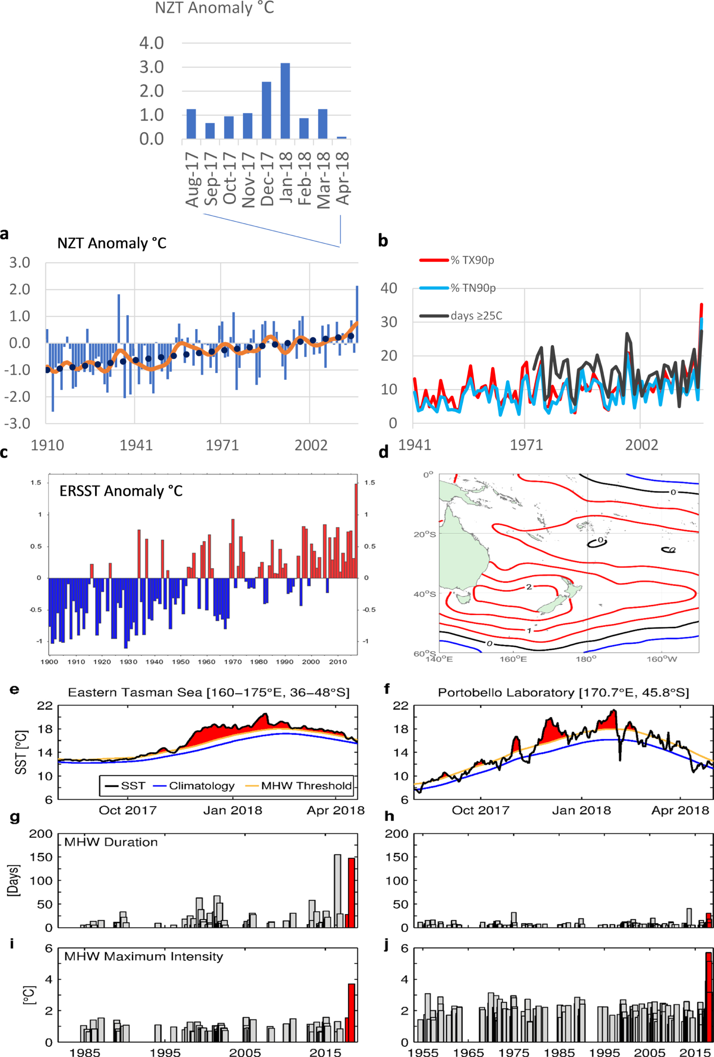
Figure 1. The 2017/18 New Zealand atmosphere and ocean heatwaves. (a) The New Zealand air temperature (NZT) series 1909–2018 summer (DJF) anomaly compared with the 1981–2010 normal. The red curve is a 15 year filtered average, and black dotted line the trend. Inset: Mean NZT August 2017–April 2018 anomalies. (b) Summer (DJF) indices of climate extremes for New Zealand from station data and VCSN. Station indices are warm days in red (percentage of time when daily maximum temperature > 90th percentile), warm nights in blue (percentage of time when daily minimum temperature > 90th percentile). The VCSN summer (DJF) count when daily maximum temperature ≥25 °C (in black). (c) Summer (DJF) SST anomalies 1900–2018 (ERSSTv5) averaged over the Tasman Sea region (26 °S–46 °S, 150 °E–174 °E) using 1961–1990 climatology (Bureau of Meteorology, Australia). (d) Composite December 2017–January 2018 SST anomalies (from NOAA ERSSTv5) using the 1981–2010 normal with contours at 0.5 ° C intervals. (e)–(j). First row: time series of summer (Dec–Feb) sea surface temperature (SST) climatology (1981–2011; blue), 90th percentile MHW threshold (orange) and summer 2017/18 SST time series (black) from (e) the eastern Tasman Sea (160–175 °E, 36–48 °S) and (f) the Portobello Marine Laboratory (45.88 °S, 170.50 °E). The red shaded regions identify periods associated with MHWs detected in the SST time series from each location using the Hobday et al (2016) definition. Second row: the duration of each MHW detected in the SST time series for (g) the eastern Tasman Sea and (h) Portobello Marine Laboratory. The red shaded bar highlights MHWs detected during summer 2017/18. Third row: as above but showing the maximum intensity of each MHW detected in the SST time series for (i) the eastern Tasman Sea and (j) Portobello Marine Laboratory.
Download figure:
Standard image High-resolution image
Figure 2. Atmospheric pressure anomalies, tropical cyclone occurrence and sub-surface temperature anomalies. (a) NCEP December 2017–February 2018 mean sea level pressure anomalies using the 1981–2010 reference period, contour interval 1hPa, negative contours blue, positive red and zero is black; (b) Named tropical cyclone (TC) tracks for the southwest Pacific for the 2017/18 austral summer to the end of April 2018 based on the latest SPEArTC dataset (Diamond et al 2012); (c) TC frequency of occurrence anomalies (right panel) calculated as the differences from the 1981–2010 climatology from SPEArTC from those TC seasons, contour interval is 0.5 TC occurrences; red contours positive; blue contours negative; zero contour omitted; (d) December 2017–February 2018 sub-surface temperature anomalies for the Pacific Ocean from 40–45°S using the 1981–2010 reference period for Global Ocean Data Assimilation System (GODAS) sub-surface temperatures; (e) regionally-averaged ARGO float measurements for the eastern Tasman Sea (35–45 °S, 160–172.5 °E) of the mean temperature anomaly over the period January 2017–May 2018.
Download figure:
Standard image High-resolution imageLand and ocean time series show that the entire New Zealand region was the warmest observed. NZT anomalies were 2.2 °C above average (figure 1(a) and table 2), the warmest on record (Salinger 1979, 1980, Mullan et al 2010). Indices of temperature extremes for New Zealand (figure 1(b) and table 2) show the highest percentage of summer warm days and warm nights above the 90th percentile (35% and 31% respectively) back to 1941. Counts of summer days ≥25 °C were the highest recorded, back to 1973. For the Tasman Sea (26°–48°S, 150°–174°E) SSTs were 1.5 °C above average (figure 1(c)), the largest anomaly on record. The biggest departures from average occurred in January, with the entire Tasman Sea/New Zealand region having a DJF anomaly of around 2 °C (figure 1(d)).
Based on both atmospheric and ocean metrics, the summer 2017/18 heatwave was the most intense on record—dating back to 1909 for NZT and 1981 for the satellite SST record. The heatwave over land developed in October and November 2017 where NZT were 1.0 °C and 1.1 °C above average respectively (figure 1(a)). December 2017 was warmer (2.4 °C) and the heatwave peaked in January 2018 with an NZT anomaly of 3.2 °C, the warmest month ever recorded. During February the event abated (NZT +0.9 °C). SSTs followed a similar temporal pattern (figures 1(e), (f)). Applying a MHW definition (Hobday et al 2016) to daily satellite SSTs from the eastern Tasman Sea, the MHW had a duration of 147 d from 14 November 2017 to 9 April 2018 (figure 1(g)), a maximum intensity of 3.7 °C (figure 1(h)), and a mean intensity of 2.1 °C (not shown, see Methods for a description of the MHW metrics). Daily SSTs from a long-term monitoring site at the PML indicated that summer 2017/18 was the warmest on record, since 1953 (figures 1(f), (j)). The DJF average temperature (anomaly) at PML was 17.8 °C (2.4 °C), 0.6 °C warmer than the previous record set in 1974/1975. Near-shore surface waters at PML were in an MHW state over four distinct periods from October 2017 to March 2018 (figure 1(f)). Of these, the 28 day period from 22 November–20 December 2017 was the most intense MHW on record at PML, with a maximum (mean) intensity of 5.7 °C (figure 1(j)) and a mean intensity of 3.4 °C (not shown).
The only other time a New Zealand coupled ocean-atmosphere heatwave of similar magnitude occurred was in 1934/35. That summer was described at the time as 'remarkably warm' (Kidson 1935) with a New Zealand-average mean temperature of 18.5 °C, 2.7 °C above the climatological normal of the day (1901–1930), and 1.9 °C above the 1981–2010 normal (Mullan et al 2010). TX90p and TN90p were 30% and 29% respectively. There was an accompanying MHW (not analysed by Kidson 1935) which developed in November 1934, became most intense in January 1935, then slowly abated. From ERSSTv5 data (Huang et al 2017), SST anomalies were 1 °C above average for the entire season surrounding New Zealand, and 2 °C off the west coast of the South Island (not shown).
Atmospheric and oceanic circulation anomalies
Atmospheric circulation anomalies for the season (figure 2(a)) show a pattern of blocking (higher than normal pressures) to the east and southeast of New Zealand, with negative pressure anomalies to the northwest of New Zealand. Over austral spring 2017 and summer 2017/2018 El Niño/Southern Oscillation (ENSO) was in a weak La Niña phase with a Southern Oscillation Index (SOI) of +0.9 in spring, and +0.0 in summer. This would on average promote a tendency towards northerly quarter airflow anomalies in spring, and northeasterly airflow anomalies over New Zealand in summer (Gordon 1986). The SAM was positive (spring +0.99, summer +1.73) especially in November (+3.2) and January (+2.7). The resultant airflow anomalies (figure 2(a)) match well with the phases of ENSO and the SAM, with the contraction of the southern westerlies towards Antarctica. The regional Trenberth circulation indices are consistent with a prevalence of northeasterly flow for the season, with negative values of both M1 and Z1 indices. New Zealand weather types show a predominance of the Block regime (observed 54.7% + 17.6%), and lack of the Zonal regime (6.6%, −18.5%) for DJF with frequent low wind situations. (figures 3(a)–(c)). The Trough regime occurrence was near normal (38.6%, +0.8%).

Figure 3. Ocean modelling: driving mechanisms for the MHW. Monthly mean values for wind speed anomaly (a)–(c), MHW intensity (d)–(f), and mixed layer depths anomaly (g–i) for the period November 2017–January 2018 based on the model hindcast. To identify MHWs the Hobday et al (2016) definition has been used. The light blue dashed box identifies the region which has been used to compute area-averages for timeseries in (j) and (k). Annual NDJ (Nov–Dec–Jan) area averaged (Tasman box) anomalies for surface heat fluxes (W m–2) and wind speeds (m s–1) are presented in (j) and SST (C) and thermocline depth (m) in (k). Mean climatological values for NDJ are given in parentheses.
Download figure:
Standard image High-resolution imageTC behaviour during the 2017/18 season was consistent with positive SOI and SAM conditions (Diamond and Renwick 2015). There was a total of eight named TCs for the full season; the 7 late season (Feb–Apr) named TCs over the southwest Pacific (figure 2(b)) were close to the expected number (6) for a late season La Niña period (Diamond et al 2013). The season's conditions may have led to an increased extratropical transition of tropical cyclones around or towards New Zealand; such a TC anomaly pattern (figure 2(c)) is consistent with both the La Niña and positive SAM state (Diamond and Renwick 2015).
The GODAS sub-surface ocean temperature pattern for DJF for 40–45°S (figure 2(d)) indicates very shallow anomalies to the west of the South Island, with a narrow band down to about 50 m east of the South Island. Argo float measurements (figure 2(e)) averaged over the eastern Tasman Sea confirmed a strong surface warming starting in December, peaking with a 3 °C mean anomaly over this eastern Tasman region. The anomaly decreased through February–April. The anomaly was shallow, mainly confined to the upper 20 m when it formed but deepened slightly as it was eroded from the surface.
Analogue seasons
A subset of past analogue three-month periods was chosen from both the NCEP and ERA-Interim reanalysis 500 hPa anomaly fields. The analogues were chosen based on the highest anomaly correlation and lowest RMS difference (RMSD) across the New Zealand/Tasman Sea region, compared to DJF 2017/18. A total of 10 ERA-Interim and 11 NCEP-I analogues were found which met threshold correlation and RMSD values as documented in table 1(a). Three-month average SOI and SAM indices were calculated for each analogue period and compared to values observed in DJF 2017/18. Both reanalyses produced very similar results in terms of SOI and SAM statistics (table 1(b)). All were associated with prominent anticyclonic anomalies of up to 60 geopotential metres (gpm) centred to the southeast of New Zealand (not shown). The positive anomalies covered an area from 25–60°S, 155°E-155°W. Compared with the analogue cases in table 1(a) (average SAM 1.19, and SOI 0.35) DJF 2017/18 was the 3rd (4th) highest SAM value for the ERA-Interim (NCEP-I) samples. The 95% significance level of SAM and SOI values for these cases is 1.63 and 0.76 respectively, based on the analogue cases in table 1(a). Hence, the SAM value (1.73) for DJF 2017/18 is statistically significant with a p-value of < 0.05, while the SOI value (0.03) was not significant so La Niña conditions likely played a minor role.
Table 1. (a) Detailed 500 hPa Analogue Results by Season (correlation threshold minimum 0.65; RMSE threshold maximum 19 gpm). These are the results of an analysis of the atmospheric circulation patterns were compared using anomaly correlation and root mean-square difference over the region 135 °E-140°W, 65 °S–25°S compared to the DJF 2017/18 season (SAM value of 1.73; SOI value of 0.03). The DJF 2017/18 SAM values were statistically significant (p, 0.05) for both ERA-Interim and NCEP I analyses. Bolded text below indicates values are p < 0.05. (b) Summary table of SAM index and SOI values and related statistics for close analogue 500 hPa height anomalies from ERA-Interim and NCEP I Reanalysis datasets as documented in table 1(a).
| ERA-interim | SAM value | SOI value | NCEP I | SAM value | SOI value |
|---|---|---|---|---|---|
| (a) | |||||
| JJA 1979 | 2.35 | −0.20 | NDJ 1958 | 0.90 | −0.67 |
| OND 1981 | 1.39 | 0.03 | DJF1962 | 1.39 | 1.17 |
| JJA 1985 | 0.47 | −0.07 | JAS 1969 | 1.50 | 0.73 |
| DJF 1994 | 1.54 | 0.00 | JJA1979 | 2.35 | −0.20 |
| FMA 1999 | 0.54 | 1.17 | JJA 1983 | 0.70 | −0.27 |
| MAM 1999 | 1.19 | 0.97 | JFM 1999 | 0.48 | 1.10 |
| JAS 2005 | 0.13 | −0.10 | FMA 1999 | 0.54 | 1.17 |
| DJF 2008 | 2.15 | 1.57 | JAS 2005 | 0.13 | −0.10 |
| DJF 2013 | 0.88 | −0.37 | DJF 2008 | 2.15 | 1.57 |
| JFM 2018 | 1.24 | 0.47 | FMA 2013 | 1.69 | 0.30 |
| — | — | — | JFM 2018 | 1.24 | 0.47 |
| (b) | |||||
| Variable | ERA-Interim (1979–2018) | NCEP I Reanalysis (1948–2018) | |||
| # of Overlapping Cases | 10 | 11 | |||
| Mean SAM Value | 1.19 | 1.19 | |||
| Mean SOI Value | 0.35 | 0.48 | |||
| SAM at p<.05 level | 1.55 | 1.73 | |||
| SOI at p<.05 level | 0.79 | 0.87 | |||
| Ranking of DJF 2017/18 SAM | 3rd Highest | 3rd Highest | |||
Ocean model hindcasts
Global ocean model hindcast results were used to characterize the MHW in time and space. In November 2017 the centre of the MHW was in the southern part of the Tasman Sea, and east to the Chatham Islands whereas by December the entire Tasman Sea and the region south of Chatham Rise were in MHW conditions with intensities exceeding 1 °C. In January the MHW weakened but still covered most of the Tasman Sea (figures 3(d)–(f)). The mixed layer (figures 3(g)–(i)) and thermocline depth (figure 3(j)) became significantly shallower (∼10 m and ∼40 m), due to the decrease in wind speeds over this period (figures 3(a)–(c)) as suggested by the MSLP anomalies. Wind speeds were around 0.5 ms−1 lower than normal during the season over the Tasman Sea, with climatological values in the order of 6–7 m s−1, reflecting a drop of around 30%. The consequence was anomalous low vertical mixing and surface warming, while the broader oceanic heat content was not affected. Area averages over the Tasman Sea (figure 3(j)) suggest that NDJ wind speeds were a record low, while surface heat fluxes were in the normal range. The subsequent lack of vertical mixing caused the SSTs to exceed previous records. This mechanism contrasts with the 2015/16 reported MHW (Oliver et al 2017), where horizontal heat advection by the EAC was identified to be the driver.
The heat wave during the austral summer period appears to be the result of coupled ocean-atmospheric processes discussed above, with the atmospheric process most likely driven by the intensity of the positive phase of the SAM.
Southern Alps ice volume and seasonal snow
Glacier volume changes in the Southern Alps for the period 1962–2018 were estimated from variations in EOSS indices. The ice volume loss in the Southern Alps in 2017/18 was 3.8 ± 0.6 km3 water equivalent (w.e.), the largest annual volume loss of permanent ice in the last 57 years (figure 4(a)). Between 1962 and 2018 the volume of ice in the Southern Alps decreased from an estimated 60.5–37.3 km3 w.e., with the 23.2 km3 w.e. change equal to a 38% loss of ice. The summer heat wave in 2017/2018 was responsible for a 9% reduction in total ice volume in the Southern Alps compared to the previous year (2016/17). The estimate for glacier loss in 2017/2018 was compared to an approach using MODIS observations of surface albedo at Brewster Glacier, which yielded a Southern Alps ice volume loss of 3.1 ± 0.7 km3 w.e. MODIS albedo observations revealed the fast and uninterrupted depletion of the winter snowpack compared to the long-term trend (figure 4(b)), leading to an early exposure of glacier ice in mid-December 2017. Surface albedo decayed further (lowest since 2000) and the snowline rose to a level close to or above the altitude of the highest point on the glacier. The minimum albedo corresponded to an annual surface mass balance value of −2.2 m w.e. on Brewster Glacier, which is the most negative surface mass balance value since 1977.

Figure 4. Southern Alps ice volume and seasonal snow. (a) Southern Alps ice volume change (km3 of water equivalent), between years, for all glaciers of the Southern Alps from 1962 to 2018. (b) Mean (blue) MODIS glacier-wide albedo (2000–2013) and the 2017/18 season (black). Light shading indicates the maximum and minimum range, and dark shading the 25–75 percentile range. (c) estimated water stored as seasonal snow (mm) from SnowSim for the period 1987–2016. The year from 1 Apr 2017–3 Mar 2018 is shown as the blue line.
Download figure:
Standard image High-resolution imageDuring the 2017–18 snow year, the SnowSim model (figure 4(c)) showed that the estimated water stored as seasonal snow leading up to August and from mid-December 2018 was the lowest on record. From mid-January it became 'negative', indicating all the seasonal snow had melted, with extraordinary loss of permanent glacier snow and ice. The satellite record corroborates this exceptional loss in snow cover compared to previous years.
Managed ecosystems: viticulture
Sauvignon Blanc flowering, véraison (soluble solids (SS) of 8 °Brix) and maturation SS of 20 °Brix dates estimated by grapevine phenology (GFV) modelling for four major New Zealand wine-growing regions (Gisborne and Hawke's Bay—both east of North Island, Marlborough and Central Otago—inland southern South Island) showed an advancement in véraison and maturation dates. The Marlborough 2017–18 growing season, particularly from mid-December, experienced temperatures far above the long-term average (figure 5(a)). The estimated dates of véraison and maturation (figure 5(a)) were 2 February and 4 March, compared to the long-term averages (1947–2017) of 15 February and 21 March (advanced by 13 and 17 d respectively). Although 2018 was the warmest season overall and ripening temperatures amongst the warmest since 1947 (Trought et al 2016, figure 5(b)), the highest mean ripening temperature occurred in 1998. t. While the GFV model dates for 20 °Brix indicated an early maturation, the compressed flowering and an exceptionally successful fruit set and higher than average potential yield experienced during the 2017/18 season delayed the harvest. Above-average bunch numbers are predicted for 2019 reflecting warmer temperatures at bunch initiation.

Figure 5. Marlborough Sauvignon Blanc grapevine maturity modelling. (a) Degree day anomaly from the long-term average accumulated degree days (base 0 °C) from 29 August. Estimated flowering (F), véraison (V) and 20 °Brix (20) dates using the Grapevine Flowering and Véraison (GFV) model. The date of the phenological events F, V and 20, reflects the degree day anomaly (i.e. the greater the anomaly, the earlier phenology–diagonal lines). The harvest year is the latter year from the austral spring to summer period. (b) Mean daily temperature from estimated véraison to estimated 20 °Brix maturation (GFV modelled values) for Marlborough, New Zealand for harvest years 1947–2018.
Download figure:
Standard image High-resolution imageMarine ecology
In southern New Zealand, extensive canopies of the habitat-forming kelp Macrocystis pyrifera were unusually absent. The 18 °C–19 °C temperature tolerance threshold of M. pyrifera (Hay, 1990) was breached three times at PML (figure 1(f)) and in a nearby open coast kelp forest, a threshold exceeded only seven times since 1953. Periods of high temperatures have been associated with regime shifts and loss of kelp forests elsewhere (Wernberg et al 2016). Significant salmon (Oncorhynchus tshawytscha) stock mortality was reported in the Marlborough Sounds, the country's most important salmon aquaculture area (Eder 2018) with importation of Atlantic Salmon (Salmo salar) for the first time (Hulburt 2018). Out-of-range reports of tropical and warm-temperate fish were also common over the summer (Ainge Roy 2018; Lewis 2018). Commercial fishers trawling for snapper (Pagrus auratus) in the north of the South Island since 1981 estimated the species had spawned six weeks earlier than normal (Morton 2018). For salmon farms in southern New Zealand SST was above 17 °C for January: only a slight increase in mortalities resulted (J. Swart pers. comm).
21st century climate scenarios comparison
Late 21st century climate change projections for New Zealand representative concentration pathways (RCPs; van Vuuren et al 2011) of 2.6, 4.5, 6.0 and 8.5 were compared with DJF 2017/18 (table 2). For example, for Northland, there were 33.4 d (averaged over all VCSN grid-points within the Northland Regional Council boundary), compared to 20.4 d in the 1981–2010 climatology, a difference of 64% above climatology.
Table 2. Statistics of summer temperature percentiles and extremes for the 2017/18 summer and for the RCPs for 2081–2100, shown separately for each New Zealand Regional Council region (following table 6 of Mullan et al 2016). Column 2 shows the model ensemble-average change in mean temperature and (in brackets) the 5th–95th percentile range over 18–41 models (dependent on RCP). Columns 3 and 4 show the percentage of time the 2017/18 daily maximum and minimum temperatures, respectively, were above the 1981–2010 90th percentiles. Column 5 gives the observed 2017/18 anomaly relative to 1981–2010. Columns 6–8 show days ≥25 °C from the VCSN for 2017/18 (column 6), 1981–2010 climatology (column 7), and percentage difference (column 8). Columns 9–12 show days ≥25 °C for the scenarios, expressed as the percentage change of 2081–2100 days relative to 1986–2005 days, for four RCPs (2.6, 4.5, 6.0 and 8.5) respectively. The map of regional council areas can be found at: http://localcouncils.govt.nz/.
| Region | Summer 2081–2100 change 1986–2005 ( °C) | 2017/18%TX90p | 2017/18%TN90p | 2017/18 mean temp. anomaly °C | 2017/18 days ≥25 °C VCSN | Average days ≥25 °C VCSN | 2017/18 Diff. % | RCP 2.6 summer change % | RCP 4.5 summer change % | RCP 6.0 summer change % | RCP 8.5 summer change % |
|---|---|---|---|---|---|---|---|---|---|---|---|
| Northland | |||||||||||
| rcp 8.5 | 3.3 (2.4, 5.0) | 37 | 27 | 1.7 | 33.4 | 20.4 | 64% | 52% | 125% | 175% | 305% |
| rcp 6.0 | 2.0 (1.4, 3.3) | ||||||||||
| rcp 4.5 | 1.5 (0.9, 2.5) | ||||||||||
| rcp 2.6 | 0.7 (0.4, 1.3) | ||||||||||
| Auckland | |||||||||||
| rcp 8.5 | 3.3 (2.3, 5.1) | 46 | 32 | 2.0 | 42.1 | 17.0 | 148% | 56% | 142% | 201% | 355% |
| rcp 6.0 | 2.0 (1.2, 3.6) | ||||||||||
| rcp 4.5 | 1.5 (0.8, 2.6) | ||||||||||
| rcp 2.6 | 0.7 (0.2, 1.4) | ||||||||||
| Waikato | |||||||||||
| rcp 8.5 | 3.3 (2.2, 5.3) | 44 | 9 | 2.0 | 39.2 | 20.5 | 91% | 41% | 103% | 144% | 256% |
| rcp 6.0 | 2.0 (1.1, 3.8) | ||||||||||
| rcp 4.5 | 1.5 (0.7, 2.7) | ||||||||||
| rcp 2.6 | 0.7 (0.2, 1.4) | ||||||||||
| Bay of Plenty | |||||||||||
| rcp 8.5 | 3.3 (2.3, 5.0) | ||||||||||
| rcp 6.0 | 2.0 (1.2, 3.6) | 24 | 40 | 2.0 | 25.6 | 14.5 | 77% | 54% | 137% | 197% | 364% |
| rcp 4.5 | 1.5 (0.8, 2.6) | ||||||||||
| rcp 2.6 | 0.7 (0.2, 1.3) | ||||||||||
| Taranaki | |||||||||||
| rcp 8.5 | 3.3 (2.2, 5.2) | 52 | 35 | 2.4 | 17.1 | 5.8 | 195% | 71% | 203% | 309% | 634% |
| rcp 6.0 | 1.9 (1.0, 3.9) | ||||||||||
| rcp 4.5 | 1.5 (0.7, 2.7) | ||||||||||
| rcp 2.6 | 0.6 (0.1, 1.4) | ||||||||||
| Manawatu- Whanganui | |||||||||||
| rcp 8.5 | 3.3 (2.3, 4.7) | 46 | 38 | 2.4 | 34.1 | 15.5 | 120% | 38% | 97% | 138% | 252% |
| rcp 6.0 | 1.9 (1.0, 3.6) | ||||||||||
| rcp 4.5 | 1.5 (0.7, 2.7) | ||||||||||
| rcp 2.6 | 0.7 (0.1, 1.4) | ||||||||||
| Gisborne | |||||||||||
| rcp 8.5 | 3.2 (2.3, 4.6) | 20 | 20 | 1.8 | 21.1 | 19.1 | 10% | 33% | 80% | 113% | 212% |
| rcp 6.0 | 2.0 (1.2, 3.4) | ||||||||||
| rcp 4.5 | 1.5 (0.9, 2.5) | ||||||||||
| rcp 2.6 | 0.7 (0.3, 1.3) | ||||||||||
| Hawke's Bay | |||||||||||
| rcp 8.5 | 3.1 (2.3, 4.5) | 22 | 29 | 2.2 | 35.3 | 22.3 | 58% | 31% | 73% | 101% | 184% |
| rcp 6.0 | 1.9 (1.2, 3.5) | ||||||||||
| rcp 4.5 | 1.4 (0.8, 2.6) | ||||||||||
| rcp 2.6 | 0.7 (0.3, 1.3) | ||||||||||
| Wellington | |||||||||||
| rcp 8.5 | 3.1 (2.2, 4.7) | 43 | 46 | 2.2 | 33.0 | 16.7 | 98% | 31% | 75% | 105% | 199% |
| rcp 6.0 | 1.9 (1.0, 3.6) | ||||||||||
| rcp 4.5 | 1.4 (0.7, 2.6) | ||||||||||
| rcp 2.6 | 0.7 (0.2, 1.4) | ||||||||||
| Tasman-Nelson | |||||||||||
| rcp 8.5 | 3.2 (2.1, 5.4) | 47 | 37 | 2.5 | 17.1 | 10.0 | 71% | 45% | 129% | 195% | 390% |
| rcp 6.0 | 1.8 (0.8, 4.1) | ||||||||||
| rcp 4.5 | 1.4 (0.7, 2.7) | ||||||||||
| rcp 2.6 | 0.6 (0.2, 1.4) | ||||||||||
| Marlborough | |||||||||||
| rcp 8.5 | 3.1 (2.1, 4.8) | 31 | 15 | 2.2 | 20.1 | 11.8 | 70% | 38% | 95% | 136% | 270% |
| rcp 6.0 | 1.8 (0.9, 3.6) | ||||||||||
| rcp 4.5 | 1.4 (0.7, 2.6) | ||||||||||
| rcp 2.6 | 0.6 (0.1, 1.4) | ||||||||||
| West Coast | |||||||||||
| rcp 8.5 | 3.2 (1.9, 5.6) | 47 | 34 | 2.1 | 17 | 7.0 | 143% | 41% | 121% | 189% | 393% |
| rcp 6.0 | 1.8 (0.6, 4.2) | ||||||||||
| rcp 4.5 | 1.4 (0.7, 2.7) | ||||||||||
| rcp 2.6 | 0.6 (0.1, 1.4) | ||||||||||
| Canterbury | |||||||||||
| rcp 8.5 | 3.0 (2.0, 4.9) | 36 | 39 | 1.9 | 31.2 | 20.5 | 52% | 21% | 50% | 68% | 128% |
| rcp 6.0 | 1.7 (0.7, 3.7) | ||||||||||
| rcp 4.5 | 1.3 (0.6, 2.6) | ||||||||||
| rcp 2.6 | 0.6 (0.0, 1.3) | ||||||||||
| Otago | |||||||||||
| rcp 8.5 | 2.9 (1.8, 4.6) | 29 | 32 | 2.2 | 27.1 | 14.4 | 88% | 20% | 51% | 70% | 138% |
| rcp 6.0 | 1.6 (0.6, 3.6) | ||||||||||
| rcp 4.5 | 1.2 (0.6, 2.6) | ||||||||||
| rcp 2.6 | 0.5 (0.0, 1.2) | ||||||||||
| Southland | |||||||||||
| rcp 8.5 | 2.8 (1.7, 4.5) | 22 | 29 | 2.3 | 16.9 | 6.7 | 152% | 28% | 72% | 104% | 216% |
| rcp 6.0 | 1.5 (0.5, 3.5) | ||||||||||
| rcp 4.5 | 1.2 (0.6, 2.5) | ||||||||||
| rcp 2.6 | 0.5 (0.0, 1.2) | ||||||||||
| Chatham Islands | |||||||||||
| rcp 8.5 | 2.8 (1.7, 4.2) | 61 | 40 | 2.6 | |||||||
| rcp 6.0 | 1.6 (0.8, 3.5) | ||||||||||
| rcp 4.5 | 1.3 (0.6, 2.4) | ||||||||||
| rcp 2.6 | 0.6 (−0.2, 1.3) | ||||||||||
| 7-station average | |||||||||||
| rcp 8.5 | 3.1 (2.0, 5.5) | 35 | 32 | 2.2 | 27.3 (VCSN) | 14.8 (VCSN) | 84% (VCSN) | 40% | 104% | 150% | 286% |
| rcp 6.0 | 1.8 (0.9, 3.6) | ||||||||||
| rcp 4.5 | 1.4 (0.5, 2.9) | ||||||||||
| rcp 2.6 | 0.6(−0.1, 1.4) |
For the scenario projections (columns 2 and 9–12), comparisons use the IPCC convention and compare 2081–2100 relative to 1986–2005. The statistical downscaling procedure (Mullan et al 2001) calculates a future change for the mean temperature only; this offset has been applied to the VCSN daily maximum temperatures over 1986–2005, and then exceedances of the 25 °C threshold counted (following table 8 of Mullan et al 2016). Changes are expressed as the percentage increase of the 2081–2100 count above the 1986–2005 count.
The DJF2017/18, counts of days ≥25 °C compare best with end-of-century projections under RCP4.5 or RCP6.0. Changes in observed number of days ≥25 °C ranged from a 10% increase relative to climatology in Gisborne (eastern North Island) to a 195% increase in Taranaki (western North Island). In terms of the climate scenario changes, summer extremes are mostly too small under RCP2.6 and far exceed 2017/18 observations by the end of the 21st century under RCP8.5. Summer temperature departures for 2017/18 compared best with end-of-century changes under RCP4.5 or RCP6.0, where mean annual temperatures increase by 1.4 °C or 1.8 °C, respectively by 2081–2100 (table 6, Mullan et al 2016).
We recognize that 2017/18 is a single-season transient extreme event, whereas conditions in the 2090s (2081–2100 average) under future scenarios are closer to a near-equilibrium state. The scenario changes in managed ecosystems and marine ecology are expected to be in the same direction as seen in 2017/18, but the changes could be larger if the drivers are consistent year after year. Larger changes are likely for slow-response components of the New Zealand climate system, such as the South Island glaciers.
Discussion and conclusions
Most global land areas have experienced more heatwaves since the mid-20th century (Donat et al 2013). Only recently have MHWs been assessed (Oliver et al 2018) and very few studies have examined coupled ocean-atmosphere heatwaves, one such example being that of Olita et al (2007) of the Mediterranean in 2003. The unprecedented heatwave in the 2017/18 New Zealand summer (DJF) was such a combined AHW/MHW event. It was the most intense on record with a maximum AHW anomaly of +3.2 °C, and MHW anomaly of +3.7 °C. The heatwave covered all the land area, the entire central and south Tasman Sea and across to 180 °E in the southwest Pacific Ocean, an area of 4 million km2. The event was discernible in monitored surface air temperatures, daily remotely-sensed SSTs, nearshore temperature loggers, GODAS and Argo float measurements. Slightly more named TCs than normal occurred in the southwest Pacific, with an above average number of extratropical transitions towards and around New Zealand. The ocean modelling analyses suggest, that a general lack of vertical mixing due to exceptional low winds during this period was the main driver for this MHW event, while earlier studies found that heat advection have triggered previous events in the Tasman Sea (Oliver et al 2017).
Likely climate drivers are depicted qualitatively in figure 6, with the role of AGW highlighted. Recent research using climate models by Perkins-Kirkpatrick et al (2018) suggests that the 2017/18 MHW would have been 'virtually impossible' without anthropogenic influence. However, the statistics from the 1934/35 event indicate it has occurred in the past in the observed record and was only 0.3 °C cooler. If AGW is adjusted for, it was in effect 0.2 °C warmer. Projected changes of pressure and wind for the late 21st century from climate models (Mullan et al 2016) show MSLP increases in the DJF period, especially to the south–east of New Zealand. The airflow becomes more north-easterly, and at the same time associated with more (possibly blocking) anticyclones. AGW also produces a trend towards the SAM being more positive resulting in higher MSLPs in the New Zealand region, and a contraction of the southern westerlies poleward, however this trend will likely be countered over the coming several decades by stratospheric ozone recovery (Arblaster et al 2011).

Figure 6. Schematic of likely driving mechanisms for the 2017/18 summer New Zealand ocean and atmosphere heatwave.
Download figure:
Standard image High-resolution image
The New Zealand DJF heatwave shows all these features (figure 6), with increased MSLP mainly from the SAM together with the oceanic and atmospheric drivers of ENSO in a weak La Niña phase. This produced very prominent positive height anomalies at the 500 hPa level with positive anomalies of up to 60 gpm centred to the southeast of New Zealand. The atmospheric circulation anomalies were associated with very low wind speeds, around 2 ms−1 lower than normal during the season. Ocean model simulations suggest this caused anomalous low vertical mixing and initiated ocean surface warming, although the broader oceanic heat content was not affected. While surface heat fluxes were normal, the lack of vertical mixing caused the SSTs to exceed previous records and led to increased temperature anomalies.
The heatwave was over land and oceanic areas, with significant impacts on the terrestrial environment and marine ecosystems. Tasman glacier snowline estimates show the highest EOSSTas on record. An estimated record 3.8 ± 0.6 km3 w.e. loss of ice occurred, the largest estimated annual volume loss of permanent ice in the Southern Alps for the last 57 years and a 9% reduction compared to the previous year. Seasonal snow storage leading up to August and from mid-December 2018 was the lowest on record. From mid-January it became 'negative', indicating all seasonal snow and some long-term ice had melted. For Marlborough Sauvignon Blanc wine grapes the 2018 season proved to be amongst the warmest since 1947, with véraison and maturation dates advanced by 13 and 17 d respectively. Unprecedented breaches of physiological temperature thresholds for habitat-forming kelp and observations of out-of-range occurrence of tropical and warm temperate fish species suggest broader impacts on marine ecosystems.
Finally, we have examined the intensity of the warming, and extreme surface air temperatures to provide a future analogue for summer climate scenarios for 2081–2100 for impact studies. The statistics of the anomalies and extremes match well with the RCP4.5 or RCP6.0 summer climate projections for the New Zealand region.
Our approach has been applied in near-real time as the event developed in the oceanic Southern Hemisphere. This contrasts with previous studies, which have separately examined AHW and MHW events (Sparnocchia et al 2006, Barriopedro et al 2011), and their physical drivers and mechanisms (Oliver et al 2018), and impacts (Benthuysen et al 2014). This also provides a useful analogue for future AGW in the region. In doing so we utilized ocean modelling to diagnose physical drivers and pioneered the use of satellite remote-sensing to track glacier ice volume loss for the Southern Alps. We note the importance of long-term observation records as well as remote-sensing observing systems to track the evolution of both AHW and MHW events. This multidisciplinary work has shown that regional heatwaves can develop rapidly and have widespread impacts on ecosystems. It would be valuable for the approach taken here to utilize both atmospheric and oceanic seasonal to interannual climate forecasting systems (Salinger et al 2016) to become part of a scheme that could provide alerts on the emergence and evolution of regional heatwaves. Under the more extreme RCP8.5 scenario, the observed 2017/18 heatwave anomalies would become typical much earlier in the century.
Acknowledgments
Updates of the Tasman Glacier end of summer snow line data to 1976 were provided by Dr Trevor Chinn. The contribution of Dr Elizabeth (Betty) Batham is recognized in establishing the long-term PML temperature record. Thanks to Dr Doug Mackie for providing the daily PML SST record used here. Observations from a salmon farm in southern New Zealand were provided by Jaco Swart, Salmon Farm Manager, Sanfords. We also thank our many colleagues and volunteers who have maintained and contributed to the New Zealand marine and climate data sets utilised in this study. Thanks to Ms Noga Yoselevich for preparing the figures. The sub-surface SST data was collected as part of the MBIE funded Coastal Acidification: Rate, Impacts and Management (CARIM) project, provided by Kim Currie. This project obtained support through the Deep South National Science Challenge.