

Abstract
KAGRA is an underground interferometric gravitational wave detector which is currently being commissioned. This detector relies on high-performance vibration-isolation systems to suspend its key optical components. These suspensions come in four different configurations, of which the type-B is used for the beam splitter and signal recycling mirrors. The type-B suspension comprises the payload, three geometric anti-spring filters for vertical isolation and one inverted pendulum for horizontal isolation. The payload comprises the optic, its marionette and their recoil masses, which hold local displacement sensors and coil magnet actuators used for damping the resonant modes of oscillation of the suspension itself. The beam splitter version has a modified lower section to accommodate a wider optical component. The payload is also equipped with an optical lever, used to monitor and control the position of the suspended optics from the ground. All four suspensions have now been installed in vacuum chambers. We describe the mechanical, electrical and control design, and the measured performance compared to requirements.
Export citation and abstract BibTeX RIS
1. Introduction
The detection of gravitational waves (GWs) from a black-hole binary inspiral event by the two LIGO detectors [1], and subsequent observations of further such events and a neutron-star binary inspiral in conjunction with the Virgo detector and non-GW telescopes [2, 3] have ushered in an exciting new era in astronomy. In order to improve the localization of sources, it is highly desirable to add further km-scale detectors to the network. LIGO-India is planned to come online on 2025 [4], and the Japanese detector KAGRA has had its first observation run together with GEO600 from the 7th to the 21st of April 2020. This run is known as O3GK and we will refer to it throughout the text. Besides improving the localization of GWs sources, KAGRA also has the goal of introducing new technologies leading to the next generation of detectors. For instance, in order to reduce the thermal noise, the test masses, which are sensitive to GWs, are cooled down to 20 K [5]. Also, the detector is built underground where the seismic motion is between 10 and 100 times lower depending on the frequency range [6].
Low seismicity allows us to design vibration isolation systems which require smaller amounts of feedback correction, thus decreasing the injected control noise, which may be harmful for the detector sensitivity. This article describes one such vibration isolation system used for the beam splitter (BS) and the three signal recycling (SR) mirrors (SR2, SR3 and SRM). Section 2 provides an overview of the different types of suspensions used in KAGRA together with requirements. Section 3 describes the mechanical components employed in the suspension and section 4 describes the sensors and actuators used locally to damp resonant modes of the suspension. Section 5 explains the topology of the control system. Section 6 reports the performance at low frequencies, where stability is important in order to acquire and keep the lock of the interferometer. Finally, section 7 reports the result of a numerical estimation of the control noise injected within the observation frequency band.
2. Overview of vibration isolation systems in KAGRA
As is standard for interferometric GW detectors, the main optics are suspended as the lowest level in a multi-stage pendulum system, which provides vibration isolation from seismic noise and minimizes the generation of thermal noise, both of which could otherwise compromise performance. KAGRA suspensions rely on passive vibration isolation at high frequencies within the interferometer observation band and active control at lower frequencies where the resonant motion of the suspension needs to be damped. Passive vibration isolation relies on the fact that the transfer function from ground motion to the load motion of a multi-stage oscillator decreases as f−2n above its resonant frequencies, where f is the frequency, and n is the number of stages. Active damping of resonant motion at low frequencies is achieved at each stage by measuring the motion and by applying forces with local sensors and actuators.
Four main types of suspensions are used in KAGRA. Figure 1(a) shows their layout and figure 1(b) shows a 3D CAD rendering of each type. Type-A suspensions [8, 9] are used for the most critical optics, namely the input and end test masses, which define the arms of the Fabry–Perot–Michelson interferometer and react to the GW. Each type-A system has an inverted pendulum (IP) stage for horizontal isolation, five stages of geometric anti-spring (GAS) filters for vertical isolation and from it hangs the cryogenic payload. [5]. Type-B suspensions, described in more detail below, are used for the BS and the three SR mirrors. They have an IP stage, three levels of GAS filters and a room-temperature payload [10]. Type-Bp suspensions are used for the three power recycling mirrors. They have two levels of GAS filters, with an extra recoil mass around the lower one as a partial substitute for an IP [7]. Type-C suspensions [11] are used for the input and output mode cleaners and are based closely on the design used for the TAMA300 interferometer [12].

Figure 1. Layout of the main optics and their vibration isolation systems used in KAGRA [7].
Download figure:
Standard image High-resolution imageThe designs of the KAGRA suspensions rely on the accumulated experience of the GW community with various seismic attenuation systems (SAS) used in other detectors and small-scale facilities [13]. In particular, they are based on the configuration of the Superattenuator used in Virgo [14], via the suspensions used in TAMA300 [11] before KAGRA. The multi-stage pendulum hangs from a pre-isolator comprising an IP and a vertical anti-spring filter. The particular implementations of the IP and GAS filters used throughout KAGRA are almost identical to those designed for a successful LIGO HAM-SAS prototype that was proposed but not adopted for the final version of LIGO [15]. Later, these devices were used in the Albert Einstein Institute ten-meter prototype [16, 17], and in the external injection bench [18] and in several other in-vacuum optical benches [19] in Virgo. The main differences between the KAGRA suspensions and the Superattenuator are the use of GAS filters [20] rather than magnetic anti-spring (MAS) filters [21] and the height of the IP and its resonance frequency. The Superattenuator IP is 6 m tall in order to provide enough height to suspend the multi-stage pendulum from the ground and is operated with a resonance frequency of around 30 mHz [14]. In KAGRA, the IP is only 0.65 m tall, and it is placed on top of a frame 3.2 m tall in type-B SAS or directly on the ground at the top of the long vertical shaft down through which the much longer pendulum of the type-A SAS hangs. The low seismic environment of the KAGRA underground allows these suspensions to reach a suitable amount of attenuation with IP resonant frequencies of around 70 mHz.
Table 1 shows the performance requirements for the type-B suspension. The damping time refers to the time it takes for the active control system to damp any resonant motion which may be involuntarily excited. The 60 s limit was set to permit quick recovery of the alignment of the interferometer. The RMS values of the longitudinal and angular displacements and longitudinal velocity concern the low frequency regime where stability is necessary to acquire and keep the optical cavity lock. These values are to be calculated by integration over all frequencies down to 10 mHz, with the dominant contributions coming from seismic noise and from the resonant motion of the suspension below 2 Hz. Finally, the displacement spectral density at 10 Hz is the requirement within the interferometer observation band.
Table 1. Required upper limits for the motion of the optics hanging from type-B suspensions [6, 22] The RMS values are to be calculated from amplitude spectral densities by integration down to 10 mHz.
| Quantity | Beam splitter | Signal recycling mirror |
|---|---|---|
| Damping time | 60 s | |
| RMS longitudinal displacement | 4 × 10⁻⁷ m | |
| RMS velocity | 5 × 10⁻⁷ m s−1 | |
| RMS angular fluctuation | 1 × 10⁻⁶ rad | |
| Displacement spectral density at 10 Hz |

|

|
3. Mechanical design of the type-B suspension
Figure 2(a) 83 shows the SR variant of the type-B suspension within the vacuum chamber and a supporting outer frame A'. The frame is in air and directly bolted onto the floor. The BS version has a payload of a different size to accommodate a wider optic and the load capacity of its upper stages is also larger. The chamber and the frame are shown in semi-transparent gray and the suspension in opaque color. The lower part of the frame and some parts of the chamber extend beyond the limits of the diagram. Figure 2(b) shows a simplified schematic cross-section showing only larger components of the multi-stage pendulum. In (a), the IP base C' in the top section of the tank is supported by the rigid frame A' from the outside of the tank via three jacks B' entering through flexible bellows, so that the frame and tank are largely mechanically decoupled at the supporting points and the height and levelness of the IP can be adjusted. The IP stage has three flexible legs D', two of which appear in the diagram, and the resonant frequency can be tuned by adding arc-shaped weights around the edge of the IP table E'. The baseline design has 172 kg of arc weights for the BS and 103 kg for the SRs. By increasing this by about 25%–35%, the resonant frequency can be adjusted to a suitable value. We require a frequency less than 80 mHz to give adequate isolation of the microseismic peak. A frequency of 40 mHz is achievable with some care but does not leave enough margin for small temperature changes and we generally work around 65 mHz. The IP has three assemblies F' arranged circumferentially around the outside, each one comprising an (LVDT) linear variable differential transformer displacement sensor and a coil-magnet actuator. Next to each LVDT/actuator assembly there is a horizontal fishing rod (FR) unit, with a pair of soft, opposed, auxiliary springs (whose curve resembles that of a fishing rod) on a motor-driven base to apply DC position adjustments. Figure 3 shows the horizontal FR for the BS suspension IP. The IP also has three geophones G' (velocity sensors) arranged circumferentially around the edge of the IP table. All these components are used to sense motion and actuate along the longitudinal (L), transverse (T) and yaw (Y) degrees of freedom of the IP.
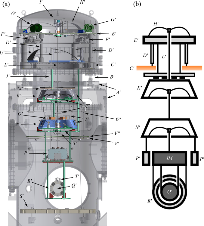
Figure 2. The 3D-CAD of the type-B suspension (SR variant) is shown in (a). A': supporting outer frame, B': jack, C': IP base, D': IP leg, E': IP table, F': LVDT, coil-magnet actuator and horizontal fishing rod, G': geophone, H': top GAS filter blades, I': various components (see text), J': security structure, K': standard GAS filter F1, L': maraging steel rod, M': magnetic damper, N': bottom Filter, O': moving masses to adjust BF pitch and roll, P': IRM, Q': mirror or beam splitter, R': RM, S': optical table, T': cable clamps, U': spring blade assemblies for the optical table suspension, V': magnetic damper for the optical table suspension, V'': iron ring with magnets, W': suspension point (see text). Figure (b) shows a simplified schematic cross-section.
Download figure:
Standard image High-resolution image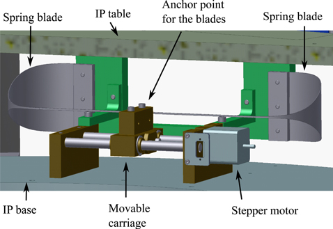
Figure 3. Horizontal fishing rods are used for coarse positioning of the IP with respect to the ground. The wide ends of the blades are fixed to the IP table whereas the thin ends are anchored to the carriage of the stepper motor mounted on the ground.
Download figure:
Standard image High-resolution imageThe top GAS filter (F0) H' is mounted on the movable IP table and supports the hanging chain, while the security structure (SS) J', which surrounds and protects the chain, is attached to the fixed underside of the IP C'. The assembly I' comprises the keystone, a motor-driven rotary bearing to allow yaw adjustments of the chain, an LVDT for sensing vertical displacement, a coil magnet-actuator and a vertical motor-driven Fishing Rod for DC position adjustment. The keystone is a component at the geometrical centre of the GAS filter structure onto which all the spring blades are clamped [20].
The second GAS filter K', called the Standard Filter (SF, a.k.a. F1), is suspended by a maraging steel rod L' from the keystone of F0. The end segments of the rod are 3 mm thick. The term 'standard' refers to the structure of all the filters that are neither on the IP table nor at the bottom interfacing with the payload. In type-B we have only one of this type of filter but as shown in figure 1, in type-A suspensions four are used. Suspension rods are thinner at the ends in order to achieve a more convenient position of the effective bending point produced under the tension of the load [23], and their tips have cylindrical nail heads that hook into cylindrical cavities [10]. As it will be described in section 6 this particular SF has two ring segments of copper plates M' on its upper surface, which interacts with a ring with magnets hanging via thin rods from the underside of the IP table E' to give eddy-current damping of the fundamental yaw mode and other pendulum modes of the chain. This sub-assembly is called the magnetic damper (MD).
The third GAS filter N', called the bottom filter (BF), is suspended with a maraging steel rod from the SF. At the hooking ends, the rod has a thickness of 2.5 mm. The BF has four large sliding masses O' on the top surface, two motor-driven, to allow for pitch/roll adjustment of the BF, and a motor-driven rotary bearings in its keystone to allow yaw adjustments of the IM stage below.
All the GAS filters have configurable numbers of blades. All BF and F0 units use three blades but with different widths according to load. The SFs in the SR suspensions use four blades whereas the one for BS uses six due to the heavier load. GAS filters F1 and BF also have LVDT displacement sensors, coil-magnet actuators acting on the keystones, and vertical motor-driven fishing rods for DC position adjustment.
From the BF hangs the payload. The IM (intermediate mass) is suspended by a central maraging steel rod from the keystone of the BF, and the intermediate recoil mass (IRM) P' is suspended by three thin rods from the base of the BF. At the hooking ends, the central rod has a thickness of 2 mm and the other three rods have uniform thickness of 2 mm. As shown in figure 4(a) the IRM encloses the IM on the top and sides. A section of the IRM has been removed from the diagram in order to show the IM and the wire clamp, which is shown in more detail in figure 4(b). The IM works as the marionette of the optic. On the inside it has two motor-driven sliding masses to allow for pitch and roll adjustments independent of the IRM, whose pitch, roll and yaw track the BF. Details of such system can be found in reference [10]. The IRM holds six displacement sensors, each one paired with a coil-magnet actuator into a unit called OSEM, which stands for optical sensor and electromagnetic actuator [24]. They measure displacement and actuate along the longitudinal (L), transverse (T), vertical (V), roll (R), pitch (P) and yaw (Y) degrees of freedom. As will be explained in more detail in section 4.1, the displacement sensor is a shadow sensor in which a flag mounted on the moving IM obstructs the path between an LED and a photodiode. The coil acts on a magnet in the flag assembly mounted on the IM. OSEMs are used for actively damping the resonant motion of the suspension. From the viewpoint shown in figure 4(a) four OSEMs are clearly visible, a fifth one is at the back side of the IRM and the sixth one is on the section which was removed from the diagram to show the IM.
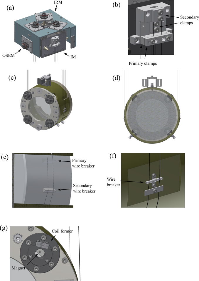
Figure 4. Some details of the SR payload.
Download figure:
Standard image High-resolution imageAs shown in figure 2 the optic (BS or SR2/SR3/SRM) Q' and the RM (Recoil Mass) R' both hang from the IM. As suggested in figures 4(a) and (c) they are both suspended by two loops of wire held by clamps at the IM, one of which is shown in figure 4(b). A double clamp arrangement is used: the primary clamps are tightened to a modest torque (2 Nm) to locate the wire, and the secondary clamps are tightened rather more firmly (10 Nm, the maximum recommended for the M6 screws) to support the load. A cross-section in figure 4(d) illustrates how the optic is nested inside the RM. The wires for the optic go through slits in the RM and reach the wire standoffs shown in figure 4(e). The standoffs are modelled on the aLIGO design: each side of the optic has a sapphire prism with two laser ablated grooves for the primary standoff, and a similar prism of machined stainless steel for the secondary. Both sets are applied with master bond EP30-2 adhesive with 5% by weight of silica beads with a diameter of 120 μm, added to reduce the risk of cracks from temperature changes [25]. As depicted in figure 4(f) the RM uses a simple grooved cylindrical metal wire standoff and a PEEK clamp. For hanging the BS and SR optics 0.3 mm and 0.2 mm diameter piano wire is used respectively and for the RMs 0.65 mm and 0.60 mm diameter tungsten wire is used for BS and SR respectively. The piano wire employed was manufactured according the JIS SWP-A norm, which allows the alloy to have between 0.80% and 0.85% of carbon, which is similar to C85 steel. The particular lot used had 0.82% of carbon.
The RM mostly encloses the optic except at the front and back, and has four coils that act on magnet-standoff assemblies attached to the optic using EP30-2 with beads as above. This arrangement is shown in figure 4(g). The original design called for four full OSEMs with displacement sensors on the RM, but the magnet-flag assemblies needed to be very long and proved impractically easy to damage, so we elected to eliminate the shadow sensors and flags and rely on the optical lever (OL) for longitudinal, pitch and yaw position sensing. This allowed us to greatly reduce the area of adhesive and increase the freedom of movement before there was risk of touching.
Cables are guided to the upper part of the chamber following paths close to the axial centre of the suspension in order to minimize the possible torques they may apply. Some of the clamping points are labeled T' in figure 2. Only a few are shown but there are many in all stages. The importance of robust cable clamping and routing is due to the fact that the suspension is very soft and small changes in the position of the cables may easily produce an unwanted displacement of the optic. Such changes may be produced by an accidental excitation from the control system or by an earthquake. Along the suspension the cables are clamped around the stages and are fixed on cable clamps which attach to the suspension rods. Cables are routed so as not touch each other or other components between clamping points, and when going from a clamping point on the suspension rod to an upper stage a particularly large amount of slack was given in order to avoid introducing any additional stiffness.
The optical table S' shown in figure 2 supports auxiliary optical components like scattered-light baffles, and injection and pick-up mirrors. Each such table has its own separate suspension. At the top are three copper-beryllium spring blades indicated by U, from which the copper ring V' hangs. The ring V' is set in close proximity of ring V'', which has magnets on its lower side and hangs from from hooking points W' on the vacuum chamber. The optical table hangs from ring V', and eddy-current damping between the rings passively damps the resonant motion of the whole optical table suspension.
An important parameter of the IM marionette is the coupling from translation degrees of freedom to rotational ones. In the nominal mechanical design of the IM, the vertical position of the centre of mass (COM) coincides with the horizontal plane of actuation of the OSEMs, configuration which is expected to minimize the couplings. However, in the real system such a coincidence does not happen due to manufacturing tolerances and also as a consequence of having to use additional ballast mass on the IM in order to reach the load the upper BF requires. In principle, during assembly the coupling can be measured when applying forces onto the IM with the actuators, and then minimized by changing the distribution of mass of the IM [26]. However, the IRM encloses the IM almost entirely, configuration that prevents further manipulation of the ballast masses once the IRM has been assembled with the OSEMs. Given this constraint, the strategy has been to reduce the actuation couplings in software by calculating a diagonalization transformation in which additional forces and torques are applied in order to reduce the coupling displacements [27]. In a prototype experiment previously reported [10], the coupling factors from longitudinal to all others DoF were reduced to less than 0.01 in units of either μm/μm or μrad/μm at frequencies of a few tens of mHz. In the case of the mirror, the wire prism standoffs were glued in line with the COM in longitudinal and vertical. Due to the wedges of the mirrors, the COMs do not coincide with the transverse geometrical centres. For instance, in SR2 the COM is nominally off by 1.5 mm. The COM of the RM does coincide with the geometrical centre. The separation between the wires holding the mirrors is 10 mm and for the ones holding the RM it is 20 mm. For O3GK, diagonalization of the IM and RM DoF was not carried out due to time constraints.
A list of resonant modes and their graphical representations can be found in reference [6, pp. 176 and 209]. The particular values of the resonant frequencies there reported correspond to a generic type-B system with nominal values of its parameters and may differ slightly from the ones reported in the following sections, which correspond to a particular realization of the suspension.
4. Sensors and actuators for control
As pointed out in section 2 the vibration isolation system relies on local sensors and actuators to actively damp the resonant motion of the suspension. For the purposes of active control, all the motor-driven adjustments (fishing rods, moving ballast masses, rotary bearings etc) mentioned above are considered fixed, and only the non-contacting sensors and actuators are used. These sensors are three L-4C geophones from Sercel and three LVDTs with coil-magnet actuators at the IP [28, 29], one LVDT with coil-magnet actuator at each of F0, F1 and BF, six OSEMs at the IM, and four coil-magnet actuators plus an OL mounted on the ground for the optic. The number of sensors and actuators were chosen so they could be diagonalized to L (longitudinal), T (transverse), V (vertical), R (roll), P (pitch) and Y (yaw) at the IM; L, T and Y at the IP; and L, P and Y at the optic; the damping then is calculated in the diagonalized basis. For the most part the diagonalization is straightforward, being based on the known geometry of the sensors and actuators, but that for the OL is more involved and is described in section 4.3. Additionally, for the IP, the position signals from the LVDTs and the velocity signals from the geophones are combined via frequency-dependent blending to give lower-noise position signals. The LVDTs are known to be more sensitive sensors at low frequencies where active control is necessary to suppress position drifts. See section 5 for more details on the control system. This section describes the OSEMs, LVDTs and geophones.
4.1. OSEMs
Each OSEM has a coil for magnetic actuation and the LED and photodiode of a shadow sensor for displacement. A cross section view is shown in figure 5(a). Six OSEMs are used on the IRM. At corresponding positions on the IRM there are PEEK pedestals, each holding an actuation magnet and a thin, flat, aluminium shadow-sensor flag. The dimensions are chosen so that when the flag tip is midway between the LED and photodiode, the magnet is at the point of maximum field gradient of the coil. The flag assembly is self-assembling via the force of the magnet on ferromagnetic inserts in the flag base and pedestal tip, which makes them resistant to permanent damage in the case of a knock. Each pedestal has a second, oppositely oriented magnet at the base to cancel the overall dipole moment of the IM. As shown in figure 4(a), each OSEM is mounted on a panel with screws that have in-out range for adjusting its position with respect to the tip of the flag. In turn, each panel is mounted on the IRM with screws in oversized holes that provide range for lateral alignment. Both types of adjustment happen after the masses are hung. Before installation in the suspension, each OSEM was calibrated in an optical table by moving a dummy flag with a micrometer. This process yields the calibration factor, typically in units of displacement per count of the ADC, and the linear range in units of displacement. The displacement sensitivity
85
of some OSEMs were also measured by rigidly fixing the OSEM body and the flag at nominal relative positions. Across the 24 OSEMs in all type-B, most have linear ranges close to 800 μm and 870 μm with one outlier at 750 μm and two at 950 μm. Figure 5(b) shows the displacement sensitivity of six OSEMs as amplitude spectral densities. With small differences between the six samples the sensitivity is close to  at 0.1 Hz and
  at 1 Hz. Typical RMS values integrated from 100 Hz down to a few tens of mHz are close to 20 × 10−9 m.
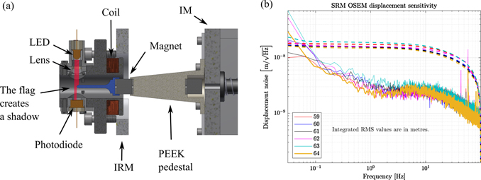
Figure 5. Diagram (a) shows how the flag (in blue) mounted on the moving IM creates a shadow on the photodiode. The plot shown in (b) is the sensitivity of the OSEMs used in SRM suspension. The labels are the OSEM serial numbers.
Download figure:
Standard image High-resolution image4.2. LVDT
LVDTs quantify displacement using the change in the mutual inductance between a single primary coil and a double secondary coil with the two halves counter-wound, which move with respect to each other [28]. Figure 6(a) shows the cross section of one of the LVDTs used in a GAS filter. This view corresponds to the region referred to as I' in figure 2. The primary coil is wound around a PEEK former attached to the keystone of the GAS filter. The coil is oriented coaxially with the suspension rod which also hangs from the keystone. The secondary coils are fixed on the GAS filter base plate. The primary coil is driven with an AC signal with constant amplitude of 5 Vpp and a frequency of 10 kHz, and the induced voltage in the secondary is demodulated using the excitation signal as a reference, and passed through a low pass filter. The resulting DC voltage is proportional to the core displacement. Figure 6(a) also depicts the coil-magnet actuator. The actuation coil is wound on the same former as the LVDT primary coil and moves together with the keystone. The magnets and an iron yoke, used to guide the magnetic field lines in a suitable manner, are fixed to the GAS filter base plate. The yoke has a central hole for the suspension rod to go through.

Figure 6. As depicted in (a) the LVDT and the coil-magnet actuator are mounted coaxially with the suspension rod. Figure (b) shows that the RMS values integrated from 100 Hz down to 1 mHz are below 200 nm.
Download figure:
Standard image High-resolution imageThe LVDT units used in type-B suspensions provide linear outputs along ranges that vary from several to many millimetres in order to accommodate the relatively large displacements that the GAS filters may experience due to their low resonant frequencies. As an example of their sensitivity, figure 6(b) shows the displacement spectral density of the six LVDTs used in the SR2 suspension. As with the OSEMs, the sensitivity was measured after locking the keystones. Some LVDTs are more sensitive than others due to differences in calibration and linear range. The least sensitive device is the one for the Top Filter with  at 0.1 Hz and
  at 1 Hz. All RMS values integrated from 100 Hz down to 1 mHz are below 200 × 10−9 m.
4.3. Optical lever
An OL is used to measure the displacement of the suspended optical component from the ground in order to damp the resonant motion of the suspension in L, P and Y, and to set its orientation in P and Y using the IM as a marionette in order to keep the alignment [30]. So far, the OL has not only been used to keep the alignment during the interferometer lock acquisition, but also during the steady state operation of the interferometer. However, in a more advanced operation stage of the interferometer steady state control system, it is planned to also use wave-front sensing because it produces signals coherent with the main interferometer beam.
The working principle of the OL is that the motion of the mirror will produce both angular and lateral displacement of a reflected light beam incident upon it, from which both longitudinal and angular displacements of mirrors can be determined. In all Type-B suspensions the plane of incidence of the OL beam is vertical. Figure 7 shows the typical propagation path of the beam in the case of the SR suspensions. The emitter optics are mounted on a breadboard located on a pylon rigidly fixed onto the floor and the receiving optics are on a breadboard fixed onto the outer frame, both sets outside of the vacuum chamber. The emitter set comprises a superluminescent diode (SLD) light source connected to a collimator via an optic fibre. At the receiving end, the OL beam reflected by the mirror is divided by a non-polarizing beam splitter and sent along two paths. One path leads directly to a quadrant photodiode (QPD), which senses primarily mirror angle (P, Y). The other path takes to a lens and then to a QPD placed at the image plane of the mirror, which senses primarily L. The three degrees of freedom can then be mathematically decoupled further in real-time.
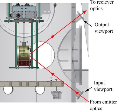
Figure 7. The plane of incidence of the OL is vertical. The beam enters and leaves the the vacuum chamber through the depicted viewports.
Download figure:
Standard image High-resolution imageIn reality, however, the optical components are not perfectly aligned and additional mechanisms of coupling between L, P and Y arise. For instance, when the beam is not reflected at the very centre of the mirror, a coupling from pitch and yaw to longitudinal appears. A detailed description of many mechanisms of coupling and methods of diagonalization can be found elsewhere [30]. Briefly, diagonalization is achieved by separately exciting in L, P and Y with white noise and examining the behavior of the different transfer functions at the resonance frequencies. For example, it is expected that at the resonance frequency for P the mirror is not moving significantly in L and Y and, therefore, any apparent coupling belongs to the sensor itself and can be removed mathematically in real time. Rather than applying an excitation at a particular frequency, white noise was used in order to distinguish resonant motion from motion produced by actuation coil imbalance as the latter is expected to be frequency independent and, therefore, its effect appears as white noise. Calibration into micrometers is achieved by measuring the position of the optical components on the breadboard and assuming 3D-CAD values for the larger and harder dimensions to measure inside the vacuum chamber. The response of the QPDs to beam displacements in micrometers was also carefully measured by moving the QPD with a micrometer stage with a still beam. After diagonalization and calibration, typical values of cross-coupling factors were approximately equal or less than 0.01 in units of either μrad/μm, μm/μrad or μrad/μrad, with a few outliers reaching 0.02 in the same units. In order to test the OL readout, the whole GAS filter chain and the payload were moved using the IP in L and Y by amounts also measured by the calibrated IP-LVDTs. The values reported by the OL and IP-LVDTs were consistent with each other within 10%. It is important to point out that the drawback of using QPDs as beam position sensors is their limited linear usable range, which affects the recovery time of the local control system when the mirrors move too far away from the centre after a large accidental excitation. For example, in the case of the SR2 suspension the linear range is approximately ±180 μm in L, ±120 μrad in P and ±180 μrad in Y. A strategy that would straightforwardly increase the angular measuring range would be to place the lens before the beam splitter, keeping the length sensing QPD at the image plane of the suspended mirror and placing the angle-sensing QPD at the focal plane of the lens [31, p 23]. This change would decrease the sensitivity, which may be an acceptable compromise.
4.4. Inertial sensors
As pointed out in section 2, the type-B system relies on passive vibration isolation within the GW observation band at 10 Hz and above. However, at lower frequencies the passive approach is not expected to be enough when intense oceanic weather increases the microseismic motion of Honshu island at frequencies of 200 mHz and below. In these conditions, active damping is necessary. Because LVDTs do not measure the IP motion with respect to an inertial reference frame but from the moving ground, the motion of the IP produced by ground motion must also be measured with an inertial sensor in order to create an appropriate feedback signal. Within a geophone the test mass is part of a harmonic oscillator subject to viscous damping. A permanent magnet is attached to the case and a pick-up coil is attached to the test mass. Relative motion between the two produces an electromotive force proportional to the velocity. As shown in figure 2, to sense motion in L, P and Y, each IP (E') uses three geophones (G'). The model used is the L-4C manufactured by Sercel. Each geophone is in air within a hermetically sealed pod that is in turn placed on the IP table in vacuum. The responsivity, defined as the transfer function from velocity to output voltage, is

in units of V (m s)−1, where ω0 is the resonance frequency of the oscillator, ζ is the damping coefficient, G is a factor that quantifies the responsivity of the pick-up coil and s is the Laplace variable [18]. For each geophone these parameters were determined with a least-square-fit of the measured transfer function from the readout of a Trillium 120QA seismometer calibrated in m s−1 to the geophone voltage output. Typical resonance frequencies are above 1 Hz, with high coherence values in the calibration measurement down to 100 mHz. The sensitivity of the geophones were also measured using a three channel correlation analysis [32]. Figure 8 shows the sensitivity of the geophones used in SR2 suspension together with a theoretical estimate of one of them [18, 33]. The predicted sensitivity takes into account the Johnson thermal noise of the resistance of the pick-up coil, the thermal noise of the inner test mass suspension and the electronic noise of an output preamplifier used to preserve the signal-to-noise ratio in the digitalization process at the ADC. The preamplifier is built with the low voltage noise operational amplifier CS3001. The theoretical calculation reveals the preamplifier noise is dominant and its amplitude coincides with a previously measured value [6, 33]. As it can be seen from the plot below 9 Hz the measured values of the geophone sensitivity are higher than the predicted ones. For instance, at 200 mHz the measured noise is larger by a factor of 3.6. We are currently in the process of identifying the source of this discrepancy. The figure also depicts the free swing displacement spectral density in IP-L measured by the geophones. The IP resonance at 70 mHz is almost completely buried in noise and the pendulum modes of the chain can be seen at 400 mHz and at 670 mHz, with the value of the noise floor consistent with the geophone noise. As will be mentioned again in section 7, such a large amount of noise did not allowed us to use the geophones during the O3GK observation campaign. In the same plot, the sensitivity of one of the IP-LVDTs is shown for the purposes of comparison.
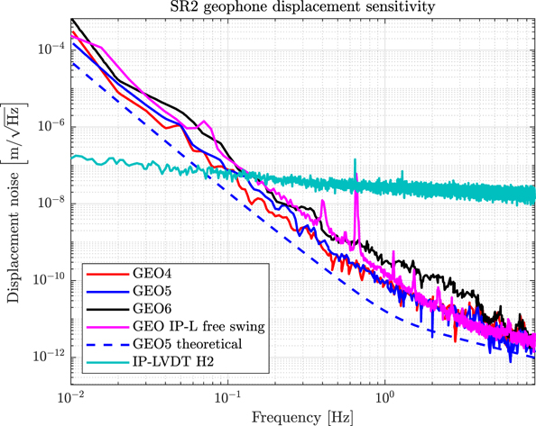
Figure 8. The measured sensitivities of the geophones are higher than expected. The measurement of IP-L free swing motion during a seismically quiet day yields a similar noise level.
Download figure:
Standard image High-resolution image5. Control system
The aim of the local control at low frequencies is twofold: to continuously keep the mirror in an appropriate position in order to allow and maintain the alignment of the interferometer, and to suppress the resonant motion of the suspension itself. Quantitatively, this means achieving a performance compatible with the requirement, listed in table 1, for the conditions in which the global control using interferometer signals are engaged and the mirrors are locked in their respective optical cavities. Besides the expected challenges posed by this goal, the control scheme faces the additional challenge of keeping the control noise injected into the interferometer observation band to an acceptable level to allow KAGRA to reach its ultimate sensitivity. In this section, local control systems that were used during O3GK are described.
Suspensions are controlled by real-time computers similar to those used at LIGO. The signals are acquired by a 16-bit analog to digital converter (ADC) at 2 kHz. In software, feedback signals are created by applying active control filters to the input signals. Using a 16-bit digital to analog converter (DAC) the feedback is then passed to coil drivers and thence to the actuators.
Each type-B suspension has fifteen DoF upon which it is possible to actuate: three at the IP (L, T, Y), one at each GAS Filter, six at the IM (L, T, V, R, P, Y) and three at the suspended optic (L, P, Y). Real displacement sensors and actuators (i.e. LVDTs in IP, shadow sensors in OSEMs and QPDs in the OL and their associated coil-magnet actuators) are mapped into these DoF via diagonalization matrices. In terms of well known categories, assuming that these DoFs are minimally coupled in both sensing and actuation, this transformation converts the multiple-input-multiple-output (MIMO) control problem to multiple single-input-single-output (SISO) problems. In this scheme the inputs are the desired values of each DoF and the outputs are their actual values delivered by the control system.
A suitable filter design must find a balance between the different competing physical elements affecting the output. Figure 9 shows block diagrams of the control system with these additional elements. The IP and the three GAS filters can be described with the same generic diagram shown in figure (a). The subscript i refers to one of IP, F0, F1 or BF. The diagram for the payload is depicted in figure (b). Parameters called out with the same letter as in (a), but with the subscripts IM and OPT, refer to analogous quantities at the IM and mirror levels respectively. Each DoF is subjected to an external disturbance Di
. At the IP and F0, the origin of the disturbance is the ground motion, and, at lower stages, the disturbance is the amount of ground motion which is not filtered out by upper stages. In diagram (a) the disturbance is explicitly represented as  , where
  is the transfer function from the displacement of the upper stage
  to the displacement of the current stage Xi
. Also, since each control loop utilizes feedback signals derived from the sensors, the signals are inevitably affected by sensor noise
to the displacement of the current stage Xi
. Also, since each control loop utilizes feedback signals derived from the sensors, the signals are inevitably affected by sensor noise  . Control loops also have setpoints Ri
to bring each stage to a position suitable for the interferometer alignment. The plant, which represents the dynamics of the system via its transfer function, is referred to as Pi
and the controller as Ki
. The controller Ki
outputs to the plant Pi
an actuation signal, which is affected by actuation noise
. Control loops also have setpoints Ri
to bring each stage to a position suitable for the interferometer alignment. The plant, which represents the dynamics of the system via its transfer function, is referred to as Pi
and the controller as Ki
. The controller Ki
outputs to the plant Pi
an actuation signal, which is affected by actuation noise  . All these blocks can be easily identified in the diagrams of the IM and mirror levels in (b). The difference is that the position of the mirror XOPT, measured by the OL, is fed into the IM control filter for DC positioning of the mirror using the setpoint ROPT.
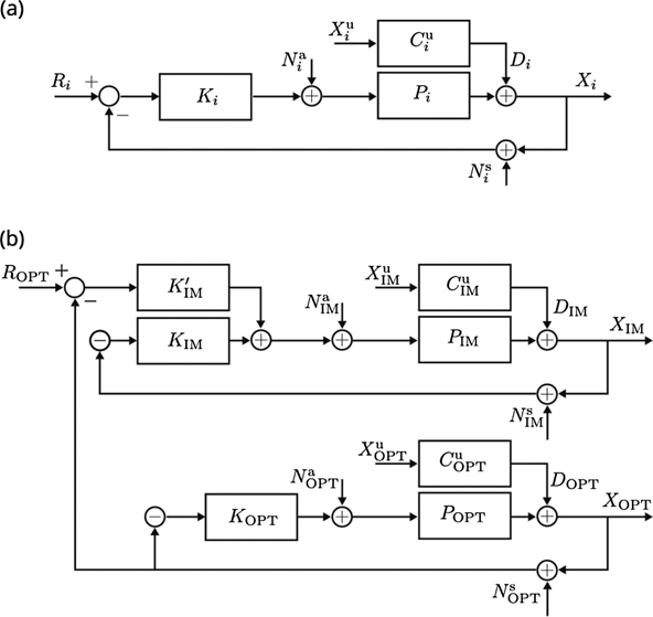
Figure 9. Block diagrams of the local control system of the type-B suspension. Diagram (a) describes either the IP, F0, F1 or BF stages. Diagram (b) describes the payload.
Download figure:
Standard image High-resolution imageThe goal is to design a filter Ki
that minimizes the coupling from the sensor noise  , actuator noise
  and from the disturbance Di
to the displacement Xi
, while keeping the displacement at the setpoint Ri
, which is typically just a DC offset. The displacement Xi
can be written as a linear combination of Ri
, Di
,
and from the disturbance Di
to the displacement Xi
, while keeping the displacement at the setpoint Ri
, which is typically just a DC offset. The displacement Xi
can be written as a linear combination of Ri
, Di
,  and
and  as
as

For DoFs with DC setpoints, the control filter includes an integrator, which has a f−1 frequency dependence and a very high gain at very low frequencies. In this frequency regime the integrator dominates over other terms present in the filter and the open loop gain Ki
Pi
≫ 1, making the displacement Xi
track the setpoint Ri
. In order to guarantee stability, the unity gain frequency (UGF) of the DC control loop is set to around 10 mHz in the IP, which is far below the frequency of the first resonance of the plant (as will be seen in figure 12). At the GAS filters the UGF of the integrator was set to around 100 mHz, lower than the resonances of the GAS filter chain, which lie between 200 mHz and 1 Hz. Stability of the stand-alone DC control loop also requires reducing the open loop gain at the resonant frequencies with notches in the filter. At higher frequencies, the displacement is dominated by the disturbance Di
, the sensor noise  and the actuator noise
  . Assuming that the disturbance and noises are not correlated, the power spectral density of the displacement reads

where the DC term related with Ri
has been dropped. It can be immediately seen that it is impossible to minimize the displacement value to zero for any control filter Ki
. This is due to the complementary nature of the coupling terms  , which means that they cannot be minimized simultaneously. Therefore, it is important to design Ki
in such a way that the control system is able to suppress the disturbance Di
while at the same time avoiding the introduction of too much noise. Resonant motion excited by the external disturbance
, which means that they cannot be minimized simultaneously. Therefore, it is important to design Ki
in such a way that the control system is able to suppress the disturbance Di
while at the same time avoiding the introduction of too much noise. Resonant motion excited by the external disturbance  and by the actuator noise
  is suppressed with damping proportional to the velocity. In frequency space this means that the filter Ki
is proportional to the frequency f. At very low frequencies this term has a negligible gain compared with the dominant integration term. As the frequency increases the open loop gain also increases such that
is suppressed with damping proportional to the velocity. In frequency space this means that the filter Ki
is proportional to the frequency f. At very low frequencies this term has a negligible gain compared with the dominant integration term. As the frequency increases the open loop gain also increases such that  at the resonances, implying that the disturbance Di
is suppressed by roughly a factor of
at the resonances, implying that the disturbance Di
is suppressed by roughly a factor of  . In these conditions, the propagated actuator noise at the output when the loop is open
  is suppressed by the same factor
  when the loop is closed, yielding a contribution of roughly
  . At frequencies higher than the resonant frequencies, the sensor noise will typically dominate since the displacement
  and actuator noise
  are both attenuated by plant transfer functions
  and Pi
respectively. With
and Pi
respectively. With  , the displacement value converges to the readout noise value. Therefore, the control filter Ki
must be rolled off with a low-pass filter such that the sensor noise coupling
, the displacement value converges to the readout noise value. Therefore, the control filter Ki
must be rolled off with a low-pass filter such that the sensor noise coupling  at the interferometer observation band, which begins at 10 Hz. In filters used for O3GK the roll-off was implemented with a few simple poles, however, an optimal implementation should use steeper low-pass filters like Butterworth or similar. The trade-off of low-pass filters is that they introduce a negative phase shift in the open loop transfer function Ki
Pi
, and this additional phase may compromise the stability if the filter cut-off frequency is too close to UGF. So, in general, the design of a suitable controller Ki
is a trade-off between disturbance rejection, noise attenuation, and stability. In general, higher-order roll-off is needed at lower stages because the control noise is not passively attenuated as much as the control noise from upper stages.
at the interferometer observation band, which begins at 10 Hz. In filters used for O3GK the roll-off was implemented with a few simple poles, however, an optimal implementation should use steeper low-pass filters like Butterworth or similar. The trade-off of low-pass filters is that they introduce a negative phase shift in the open loop transfer function Ki
Pi
, and this additional phase may compromise the stability if the filter cut-off frequency is too close to UGF. So, in general, the design of a suitable controller Ki
is a trade-off between disturbance rejection, noise attenuation, and stability. In general, higher-order roll-off is needed at lower stages because the control noise is not passively attenuated as much as the control noise from upper stages.
Displacement parameters  , Di
and Xi
are given with respect to an inertial reference frame. The LVDTs and OSEMs, however, are mounted on mechanical stages that move in a such a way that they cannot be considered inertial reference frames. In the diagrams in figure 9 the motion of the sensors themselves must be taken into account as a component of the noise
, Di
and Xi
are given with respect to an inertial reference frame. The LVDTs and OSEMs, however, are mounted on mechanical stages that move in a such a way that they cannot be considered inertial reference frames. In the diagrams in figure 9 the motion of the sensors themselves must be taken into account as a component of the noise  . Thus, the noise
  is the addition of the intrinsic readout noise (figures 6(b) and 5(b)) and the displacement of the stage upon which the sensor is mounted. In the case of the IP and F0 the LVDTs are directly mounted on the ground and, therefore, their readouts are directly affected by seismic motion. In order to prevent excessive injection of microseismc motion at the IP along L and T, the control filters were designed such that the control band does not include the frequency of the microseismic peak. As a trade-off, some resonances sensed at the IP at higher frequencies were not actively damped.
In the future, the control strategy will make use of sensor correction and sensor blending techniques. Sensor correction refers to the subtraction of the ground motion contribution from the readout of the IP and F0 LVDTs using the signal of a nearby seismometer mounted on the ground. This would allow us to use a higher gain for active isolation from seismic motion and also for damping for resonances at higher frequencies. Sensor blending refers to the simultaneous use of the LVDTs and the geophones within the IP control loop. LVDTs and geophones have different advantages over different frequency bands due to their different intrinsic sensitivities. Namely, as shown in figure 8, at low frequencies the LVDTs are more sensitive whereas the geophones are better sensors at higher frequencies. Therefore, a blended sensor uses the geophones to sense the IP motion produced by the microseismic peak at around 200 mHz and use the LVDTs at lower frequencies where the geophones are too noisy. As suggested above, above the resonant frequency of the IP the LVDTs have the additional disadvantage of being limited by ground motion because they are mounted on the ground and the IP tends to be mechanically isolated from it. The geophones, on the contrary, are inertial sensors and are not limited by ground motion. They directly measure the velocity of the IP table with respect to an inertial reference frame. At frequencies closer to the resonant frequency and below it the coupling of the IP to the ground increases making the contribution of the ground motion to the LVDT signal less important allowing us to measure the IP position with respect to the ground more effectively.
6. Performance at low frequencies
This section reports the measured performance at low frequencies during the commissioning and the O3GK observation campaigns in 2020. During this stage the aim was to achieve the minimum level of stability sufficient for the interferometer to function rather than to reach the ultimate performance of the suspension. The scope of the control system used during the measurements reported in this section did not reach the full extent described in section 5 mainly due to time restrictions. In the IP and all stages of vertical attenuation shown in figure 2, DC position control and AC damping control were implemented according to the guidelines given in section 5. The IP used only LVDTs with low control gain above the IP resonant frequencies in order to minimize the injection of ground motion. In section 7 the numerically calculated behaviour of the suspension with a more favorable implementation of the control system for the interferometer sensitivity will be reported.
The behaviour of the suspensions at low frequencies determines whether the main interferometer control system is able to acquire and maintain the lock. It also determines how fast the interferometer locking conditions can be recovered after an unlock event involving the overall suspension. Disturbances may be external, like human activity or an earthquake, or produced internally as an accidental excitation of a subsystem of the control system itself. In this frequency band the performance can be characterized by the behaviour of specific subsystems upon different conditions, all of which are described in this section.
Besides the devices used for active control described in section 4, the type-B suspension also has a passive eddy current damper [34] for the lowest yaw resonant mode of the whole chain at 55 mHz. From rigid body simulations of the whole suspension [6, 35], the amplitude of the IP motion in this mode is expected to be too small to use its sensors and actuators to damp it, yielding no actuators in the lower stages capable to do it. This torsion mode can be excited by the IP motion itself, when its amplitude is large enough, or may also be excited by the radiation pressure produced by the laser impinging on the suspended mirror [36]. As shown in figure 10(a) the magnetic damper comprises two copper ring segments fixed on top of the F1 GAS filter and an iron ring with magnets attached to its bottom in close proximity to the copper ring. The magnets are barely visible in this view but in figure 10(b) a section of the iron ring has been removed in order to show them. In figure 10(a) the three maraging steel rods holding the iron ring from the IP table are clearly seen. The height of the iron ring can be adjusted by moving the upper attachment points of the three suspension rods to the IP table. The nail heads of the rods hook into cylindrical pieces with outer threads, which are inserted into threaded holes in the table. A similar arrangement for the IM and its suspension rod is described in reference [10]. The copper segments and the iron ring are coated with nickel plating to make them UHV compatible. During assembly, outside of the vacuum chamber, the gap between the magnets and the copper segments was initially measured with a non-magnetic ruler with sub-millimetre scale and, once inside the chamber, the position of the hooks was then adjusted with a vernier caliper, yielding an uncertainty of the order of ±0.3 mm. This value is also a measure of reproducibility in the positioning of the ring among the different suspensions.
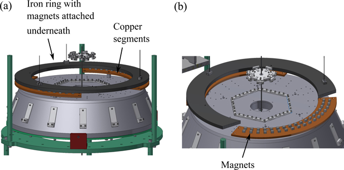
Figure 10. The iron ring, with magnets attached underneath, is depicted in (a) as it hangs right above the copper ring on top of the F1 GAS filter. In the view shown in (b) a section of the iron ring has been removed in order to show the magnets. There is a gap between the magnets and the copper ring.
Download figure:
Standard image High-resolution imageThe goal is to set the position of the iron ring with respect to the copper segments so as to achieve underdamped oscillations with a decay time below 60 s in order to yield a fast recovery of the aligned state whenever an excitation arises. Figure 11 shows the decaying yaw displacement of the mirror, measured by the OL, for three different positions of the iron ring in the SR3 suspension. The torsion mode was excited with sinusoidal actuation applied in yaw using the IP coil-magnet actuators. After waiting for a few seconds for the motion to become large enough, the excitation was suddenly interrupted and the yaw displacement was measured with the OL. The envelope of the damped oscillation was calculated using the Hilbert Transform and a decaying exponential exp(−t/τ) was fitted to the envelope where t is time and τ is the decay time. From the top plot to the bottom one, the gap between the lower face of the magnets and the upper surface of the copper ring is 8.5 mm, 5.5 mm and 3 mm with decay times of 94, 27 and 17 s respectively. The uncertainty intervals of ±0.3 mm around these positions do not overlap each other and are at least almost a couple of millimetres apart, making the nominally different gaps values meaningfully distinctive. Whereas the plot for the gap of 8.5 mm clearly shows such a configuration is not suitable, the other plots offer more interesting information about the other two configurations. In both of them the damped oscillation at 55 mHz is clearly seen together with components at higher frequencies. In the middle plot, oscillations at 149 mHz and 1 Hz are clearly seen. Both correspond to yaw modes of the IM, RM and mirror, whose decay times are reported below and which the damper ring is not designed to damp. The active control system is meant to be used instead, which during these measurements was off. In the bottom plot it is clear that the 55 mHz motion damps rather quickly making clearly visible the 1 Hz oscillation. Oscillations in the frequency neighborhood of 149 mHz can be seen below 80 s. The exact modes which were excited and their amplitudes were not reproducible in the different measurements. We remark that during the measurements reported in figure 11 the OL signals were not optimally diagonalized and, therefore, a certain amount of pitch and longitudinal displacement should be also expected to be seen in yaw. The configuration selected had the magnets on the iron ring 5.5 mm above the copper ring and a decay time of 27 s. Possibly the decay time could have been further improved but we also wanted a gap large enough to ensure the magnets and the copper plates would not touch each other during subsequent work involving the Top Filter, whose LVDT has a total linear range of ±4 mm.
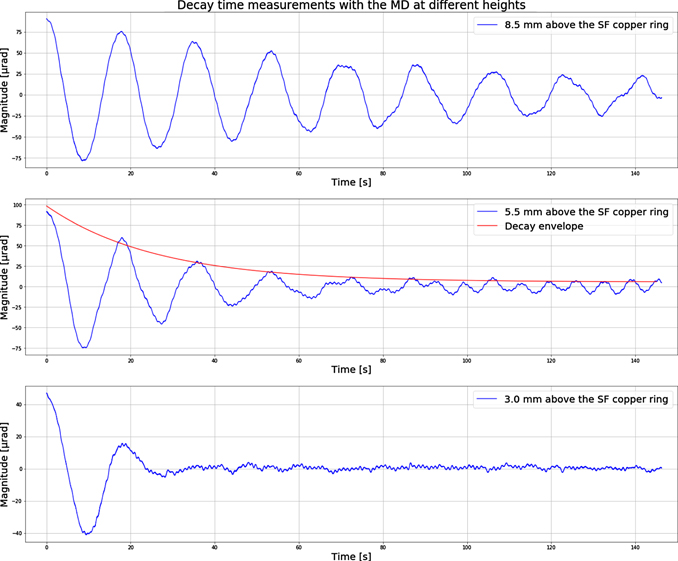
Figure 11. Torsion mode amplitude decay, measured by the OL, for different positions of the MD. The values of the height refer to the gap between the magnets and the copper ring.
Download figure:
Standard image High-resolution imageIt is worth pointing out that the effect of the residual motion of seismic origin of the damper ring is not expected to be a harmful contribution to the isolation performance nor a dominant one. The damper ring hangs from the IP table, and the effect of residual IP table motion on the overall isolation is expected to be far greater via the direct path through the main suspension rods than via the damper ring.
Besides continuously damping possible excitations produced by persistent microseismic motion the active control system also aims to damp sudden temporary disturbances after they ceased. Figure 12 shows the values of the decay times for 25 different modes according to frequency. The horizontal line indicates the 60-s limit set to achieve fast recovery of interferometer operation. The resonant frequencies were identified from force to displacement transfer function measurements with 10 mHz resolution or from free swing displacement amplitude spectral densities. The shape of each mode is reported in reference [6, pp 176 and 209]. As with previous reports [7, 10], each mode was excited with the actuators at the relevant stage and its displacement was measured with the devices described in section 4. The envelope of the damped oscillation was also calculated using the Hilbert transform and then a decaying exponential was fitted to the envelope in order to estimate the decay time. As can be seen in figure 12, with the control system on all the decay times are below the limit. The decay times of the payload yaw modes at 149 mHz and 1 Hz, which are present in the mirror displacement plots shown in figure 11, have decay times of 4.8 s and 3.5 s respectively when active damping is used. Current efforts include the blending of LVDTs and geophones in order to achieve a sensor with better sensitivity in the region of the microseismic peak and above, and also the redesign of some filters to have a higher unity gain frequency. Therefore, the decay times of some of the modes are likely to become smaller in the future.
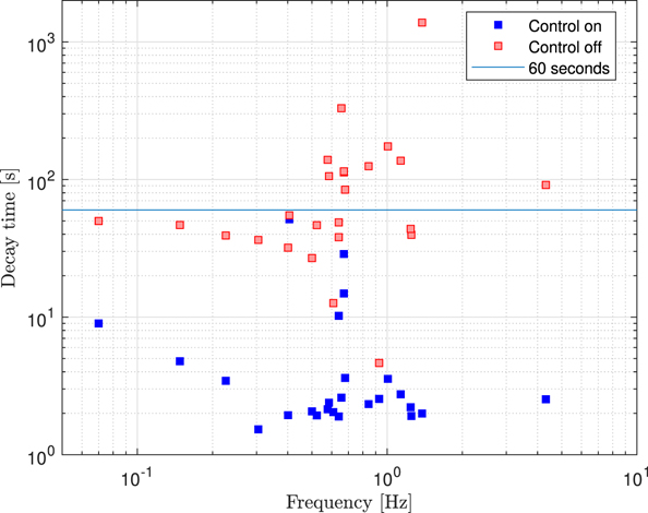
Figure 12. Decay times of 25 resonant modes of the SR2 suspension according to frequency. With the control on their values are below 60 s.
Download figure:
Standard image High-resolution imageAs stated in table 1 the RMS displacement and velocity of the mirror with the control system should be small enough to allow the lock acquisition of the interferometer optical cavity. Figure 13 shows the residual displacement and velocity of the SR2 mirror measured by the OL on March 2020 just before O3GK observation campaign, together with ground motion data. The RMS displacement integrated from 10 Hz down to 10 mHz is 2.7 × 10⁻⁷ m in L, 1.8 × 10⁻⁸ rad in P and in 6.2 × 10⁻⁹ rad in Y. The corresponding RMS velocities are 3.0 × 10⁻⁷ m s−1 in L, 6.6 × 10⁻⁸ rad s−1 in P and 1.4 × 10⁻⁷ rad s−1 in Y. All these quantities are below the requirement shown in table 1. This measurement provides upper limits above the first resonance frequency of the IP in L and T at 70 mHz. In the frequency band right above the resonance, the measurement is expected to be limited by seismic motion because the OL is mounted on the ground. However, from 700 mHz onward, the OL intrinsic noise is expected to dominate instead. At that frequency, the OL readout in L is above  and, as will be shown in figure 15(b) in section 7 and was reported in reference [6, pp 103, 104], the residual motion of seismic origin and the one produced by the OSEM sensor noise respectively, are both of the order of
  . On days of bad weather, the contribution of the microseismic motion to the readout of the OL increases. This in turn yields a higher upper limit estimate of the residual motion of the suspended mirror thus making the comparison with the requirement difficult. In these conditions the only alternative is to use the main interferometer as a displacement sensor to characterize the performance of the overall suspension.
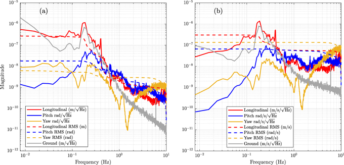
Figure 13. The RMS displacement (a) and RMS velocities (b) of the SR2 mirror measured by the OL are below the requirement listed in table 1. The apparent increase of the ground motion displacement below 60 mHz is due to noise in the seismometer.
Download figure:
Standard image High-resolution imageLong term stability of the mirror position and orientation is also important for the operation of the interferometer. Besides the obvious need to keep the orientation and longitudinal position of the optic constant, the height of the SRs should also be controlled due to the radius of curvature of the front faces of the mirrors (the BS is flat). The IPs and GAS filters are very sensitive to temperature changes due to the change of Young's modulus of maraging steel. For the Virgo Superattenuator, which uses maraging steel in its magnetic anti-spring filters, the temperature is kept within 0.2 °C [37] because those devices do not have coil-magnet actuators [14]. In KAGRA all GAS filters have coil-magnet actuators and together with the LVDTs the keystone positions are kept constant with DC control loops. In order to assess stability the hourly mean positions of the IP and GAS filters of the SR2 suspension were examined for a period of two months in which the temperature of the clean booth changed by 1.1 °C. Figure 14 shows the position values after the removal of large excursion data points which suggested the presence of an external excitation. The positions of the IP, F0 and BF do not track the temperature trend but cluster around the set point with small standard deviations, which are represented in figure 14 with red lines. For IP-L, F0 and BF the standard deviations are 81 nm, 11 nm and 36 nm respectively. F1 GAS does have a trend resembling the temperature trend but its position only changes by 17 nm during this period. These values are smaller than the integrated RMS values reported in section 4.2 because the hourly mean averages out high frequency noise which is the main contributor to the values plotted in figure 6.
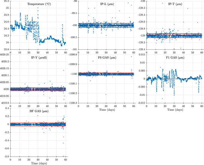
Figure 14. Hourly average of the positions of SR2 IP and GAS filters over a span of sixty days in which the temperature changed by 1.1 °C. The DC control loops keep the values around small neighborhoods with standard deviation values represented by the red lines.
Download figure:
Standard image High-resolution imageVertical stability is also affected by the thermal expansion of the suspension rods themselves, which the LVDTs cannot measure. Given the accumulated length of the three rods of 2413 mm, and the coefficient of thermal expansion of maraging steel α = 10.3 × 10⁻⁶/°C, it is easy to calculate that, under a temperature change of 1.1 °C, the mirror moves by 27 μm. Thus, with the current implementation of the control system, thermal expansion of the rods become a dominant contribution upon large temperature changes. Nevertheless, currently this is not foreseen to have a harmful influence, especially with current efforts of improving temperature control in the underground site.
7. Numerically calculated performance
This section reports the result of a numerical calculation showing it is possible to meet the requirement listed in table 1 for the residual motion of the optic within the interferometer observation band at 10 Hz and above along the longitudinal degree of freedom. The calculation is based on the rigid body model [6, 35] developed for KAGRA's suspension design. The residual motion of the optic includes the contributions of ground motion and sensor noise injected by control loops.
This calculation does not consider the damping of the microseimic peak at the IP using the currently installed geophones. Their noise level only allows blending with the LVDTs at frequencies which are too high to use them appropriately for damping at 200 mHz. Nevertheless, the frequency band in which the geophones will be used goes up to above 640 mHz where the second pendulum mode of the chain is. Because this frequency is relatively low and also because the IP is far away from the optic, the control noise injected by such a subsystem is not expected to be a problem at 10 Hz. It is worth mentioning that in a Type-B suspension prototype test in Tokyo, damping with the geophones experimentally achieved a reduction by a factor of 2 in the RMS velocity of the IP compared to the uncontrolled free swing case [6]. The numerical estimate considers a safety overall 1% coupling from the vertical degrees of freedom into the main longitudinal one including a fraction of 0.33% accounting for the 1/300 rad slope of the KAGRA tunnel. The amount of ground motion used was the 90 percentile amplitude spectral density. Figure 15(a) shows the residual motion of the mirror. The requirement at 10 Hz and above is shown in dark green and the requirement for the integrated RMS displacement is shown in orange only at low frequencies. In both cases the calculated displacement is below the requirement. The calculated integrated RMS displacement is 2.7 × 10⁻⁷ m and the displacement spectral density is  at 11.48 Hz at its closest point to the requirement value. At this frequency there is a vertical resonance of the IM, RM and optic. The control loops considered are the DC position and AC damping control for the IP using the LVDTs, DC position control for the three GAS filters and AC damping control for the F0 Top GAS filter. DC control loops have UGFs of around 10 mHz and all filters have been rolled-off to minimize the contribution of injected sensor noise. In order to allow the suspension to reach a performance compatible with the requirement using only local sensors, the use of the OL and IM OSEM displacement sensors is not considered as they introduce too much noise. The OL would introduce too much seismic noise and the intrinsic noise of the OSEMs is too high. It is worth noting that, at such frequencies, the residual motion of seismic origin of the IM relative to the the IRM, where the OSEMs are mounted, is smaller by orders of magnitude compared with the intrinsic noise of the OSEMs. In a later stage of development, we hope to either replace these sensors or mix them with more sensitive interferometric devices such as wave-front sensors and the main interferometer itself. The major contributions to the integrated RMS are the ground motion and the resonant mode just above 400 mHz
86
, both injected via the IP LVDTs. The latter is also a consequence of not using the inertial sensors for damping. The LVDTs make it necessary to limit the unity gain frequency of the IP control filter to below 100 mHz in order to avoid introducing an even larger amount of ground motion, thus leaving the resonance undamped. This condition becomes manifest in the decay times reported for this mode in figure 12. With the control on and off the decay times are above 50 s with no significant difference between the two. Figure 15(a) includes the contributions of the IP and GAS Filter sensor noise, which refers to LVDT intrinsic readout noise propagated through the control filters and the plant. The peaks in the contribution of the GAS Filter plot come from damping the modes at 218 mHz and 588 mHz. Figure 15(b) shows the simulated residual motion of the mirror with the same configuration of the control system, but calculated using the ground motion data shown in figure 13(a). The blue line is the OL measurement from the same figure, which is shown again for the purposes of comparison. At low frequencies the calculated displacement is consistent with the OL measurement given the fact that the OL is mounted directly on the ground and is therefore affected by its motion. Notice, additionally, that unlike the behaviour shown in figure 13, with the control system configuration used in the calculation, above 700 mHz the residual motion is below the ground motion.
at 11.48 Hz at its closest point to the requirement value. At this frequency there is a vertical resonance of the IM, RM and optic. The control loops considered are the DC position and AC damping control for the IP using the LVDTs, DC position control for the three GAS filters and AC damping control for the F0 Top GAS filter. DC control loops have UGFs of around 10 mHz and all filters have been rolled-off to minimize the contribution of injected sensor noise. In order to allow the suspension to reach a performance compatible with the requirement using only local sensors, the use of the OL and IM OSEM displacement sensors is not considered as they introduce too much noise. The OL would introduce too much seismic noise and the intrinsic noise of the OSEMs is too high. It is worth noting that, at such frequencies, the residual motion of seismic origin of the IM relative to the the IRM, where the OSEMs are mounted, is smaller by orders of magnitude compared with the intrinsic noise of the OSEMs. In a later stage of development, we hope to either replace these sensors or mix them with more sensitive interferometric devices such as wave-front sensors and the main interferometer itself. The major contributions to the integrated RMS are the ground motion and the resonant mode just above 400 mHz
86
, both injected via the IP LVDTs. The latter is also a consequence of not using the inertial sensors for damping. The LVDTs make it necessary to limit the unity gain frequency of the IP control filter to below 100 mHz in order to avoid introducing an even larger amount of ground motion, thus leaving the resonance undamped. This condition becomes manifest in the decay times reported for this mode in figure 12. With the control on and off the decay times are above 50 s with no significant difference between the two. Figure 15(a) includes the contributions of the IP and GAS Filter sensor noise, which refers to LVDT intrinsic readout noise propagated through the control filters and the plant. The peaks in the contribution of the GAS Filter plot come from damping the modes at 218 mHz and 588 mHz. Figure 15(b) shows the simulated residual motion of the mirror with the same configuration of the control system, but calculated using the ground motion data shown in figure 13(a). The blue line is the OL measurement from the same figure, which is shown again for the purposes of comparison. At low frequencies the calculated displacement is consistent with the OL measurement given the fact that the OL is mounted directly on the ground and is therefore affected by its motion. Notice, additionally, that unlike the behaviour shown in figure 13, with the control system configuration used in the calculation, above 700 mHz the residual motion is below the ground motion.
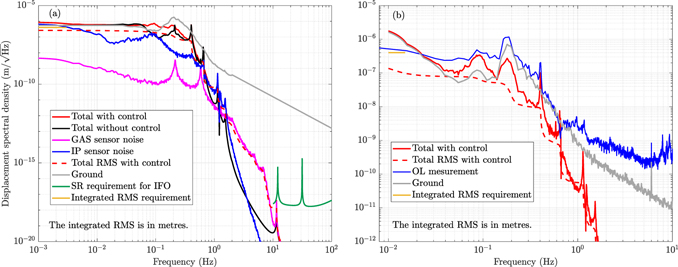
Figure 15. Graph (a) shows the calculated residual motion of the SR2 mirror. The integrated RMS motion is below the requirement of 4 × 10⁻⁷ m and the residual motion at 10 Hz is below the requirement of  . Graph (b) shows the calculated residual motion using the ground motion data reported in figure 13(a). Again, the apparent increase of the ground motion displacement below 60 mHz is due to noise in the seismometer.
Download figure:
Standard image High-resolution image8. Conclusions and future work
The previous sections describe the mechanical components of the type-B suspension, its measured behaviour at low frequencies and report a numerical estimate of the residual motion at 10 Hz where the observation band of the main interferometer begins. The higher part of the suspension comprises an IP and three GAS filters with typical resonance frequencies around 65 mHz and a few hundreds of mHz respectively at the time of initial tuning. Displacement control at each of these stages is achieved with coil-magnet actuators and LVDTs with resolutions below 200 nm. The payload comprises the suspended optic, its marionette IM and their respective recoil masses. The damping at the IM is achieved with OSEMs whose displacement sensors have resolutions close to 20 nm.
Two important features of the suspension were experimentally verified. The first is decay times of resonant motion shorter than a minute. This was achieved using active damping with LVDTs and OSEMs and passive damping with the magnetic damper ring above the standard filter F1. One minute at the longest was the requirement set for a quick recovery of the conditions necessary for interferometer alignment. The second feature is low enough amplitudes of the residual motion of the suspended mirror to allow the interferometer to acquire lock. Such a residual motion was measured with the OL at low frequencies with the control on, and its value is below the requirement shown in table 1.
Another very important requirement set for the residual motion of the mirror is having amplitudes low enough for the interferometer to reach its ultimate sensitivity at 10 Hz and above. Due to time restrictions imposed by the O3GK calendar, it was impossible to experimentally measure the mirror displacement using the interferometer as a displacement sensor. Neither was there time for the fine tuning of the control system for it to deliver low amounts of injected control noise. Therefore, in this paper we present instead a numerical estimation based on the rigid body model of the suspension using a control configuration favorable in terms of control noise. According to this calculation, the type-B suspension is indeed potentially capable of meeting the requirement shown in table 1. From the experimental point of view, however, the challenge in creating the conditions to realize such a result remain.
Diagonalization of the IM sensors and actuators is necessary. In the mirror stage only the actuators remain to be diagonalized. Increasing the measuring range of the OL would allow the control system to effectively act upon large amplitude motion. In future upgrades the damping of the IP with inertial sensors is necessary. The noise in the currently installed geophones is such that the blending frequency is too high to effectively damp the microseismic peak. Besides experimentally identifying the dominant noise source and mitigating its effect, another course of action has been the development of a more sensitive seismometer whose prototype is currently under test [38]. Performance can also be improved by the subtraction of ground motion from the IP and F0 LVDTs, as they move together with the ground, horizontally and vertically respectively. This technique is referred to as sensor correction; it has been implemented in type-A suspensions already [9] and is currently being implemented in type-B systems. Another outstanding item is the measurement of the transfer function from ground motion to optic displacement using the interferometer as a sensor.
Acknowledgments
We appreciate the contributions from Takanori Sekiguchi, Riccardo DeSalvo, Gianni Gennaro and Joris van Heijningen during the prototype development. This work was supported by MEXT, JSPS Leading-edge Research Infrastructure Program, JSPS Grant-in-Aid for Specially Promoted Research 26000005, JSPS Grant-in-Aid for Scientific Research on Innovative Areas 2905: JP17H06358, JP17H06361 and JP17H06364, JSPS Core-to-Core Program A. Advanced Research Networks, JSPS Grant-in-Aid for Scientific Research (S) 17H06133, the joint research program of the Institute for Cosmic Ray Research, University of Tokyo, National Research Foundation (NRF) and Computing Infrastructure Project of KISTI-GSDC in Korea, Academia Sinica (AS), AS Grid Center (ASGC) and the Ministry of Science and Technology (MoST) in Taiwan under grants including AS-CDA-105-M06, Advanced Technology Center (ATC) of NAOJ, Mechanical Engineering Center of KEK, the LIGO project, and the Virgo project.
Footnotes
- 83
Primed labels are used to to avoid conflict with the names of other parameters.
- 85
In this paper we call sensitivity to the smallest amount of a quantity a sensor can measure. It is determined by the total noise and is typically expressed in units of an amplitude spectral density, e.g.
 for a displacement sensor.
 - 86
This mode is #11 in reference [6].
