
DNA-Guided Assembly for Fibril Proteins

 , , , , , ,
Abstract
:1. Introduction
2. Materials and Methods
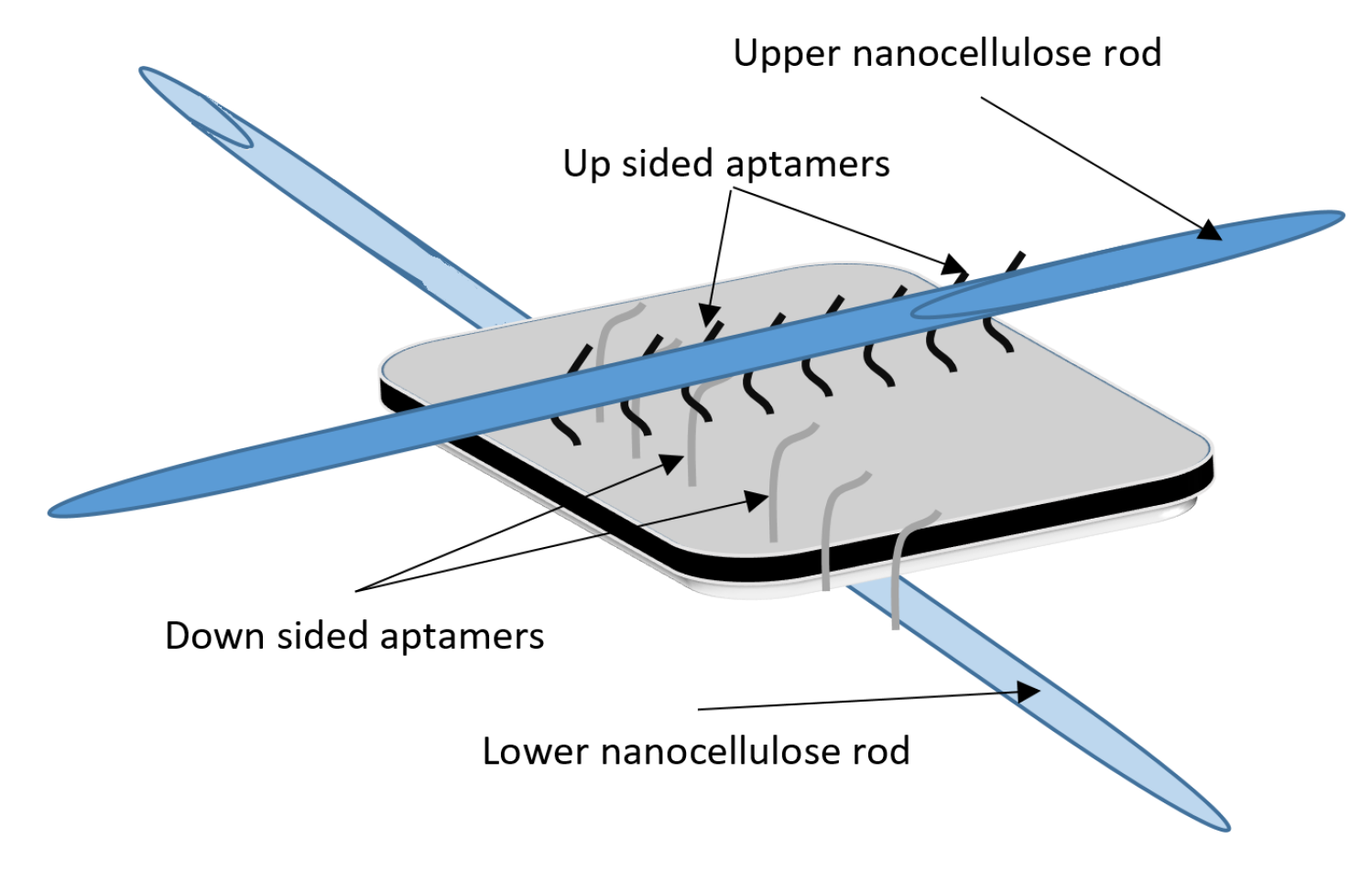
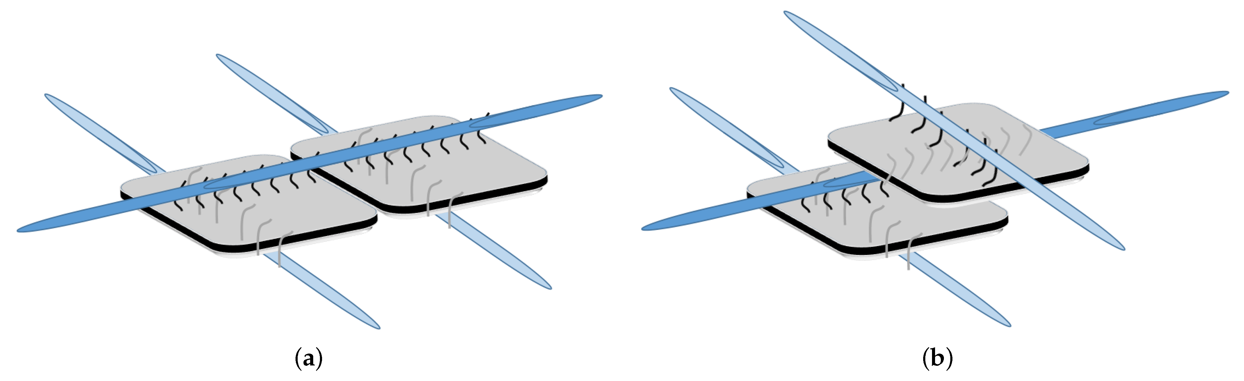
DNA-Guided Assembly of Nanocellulose Meshes
3. Results
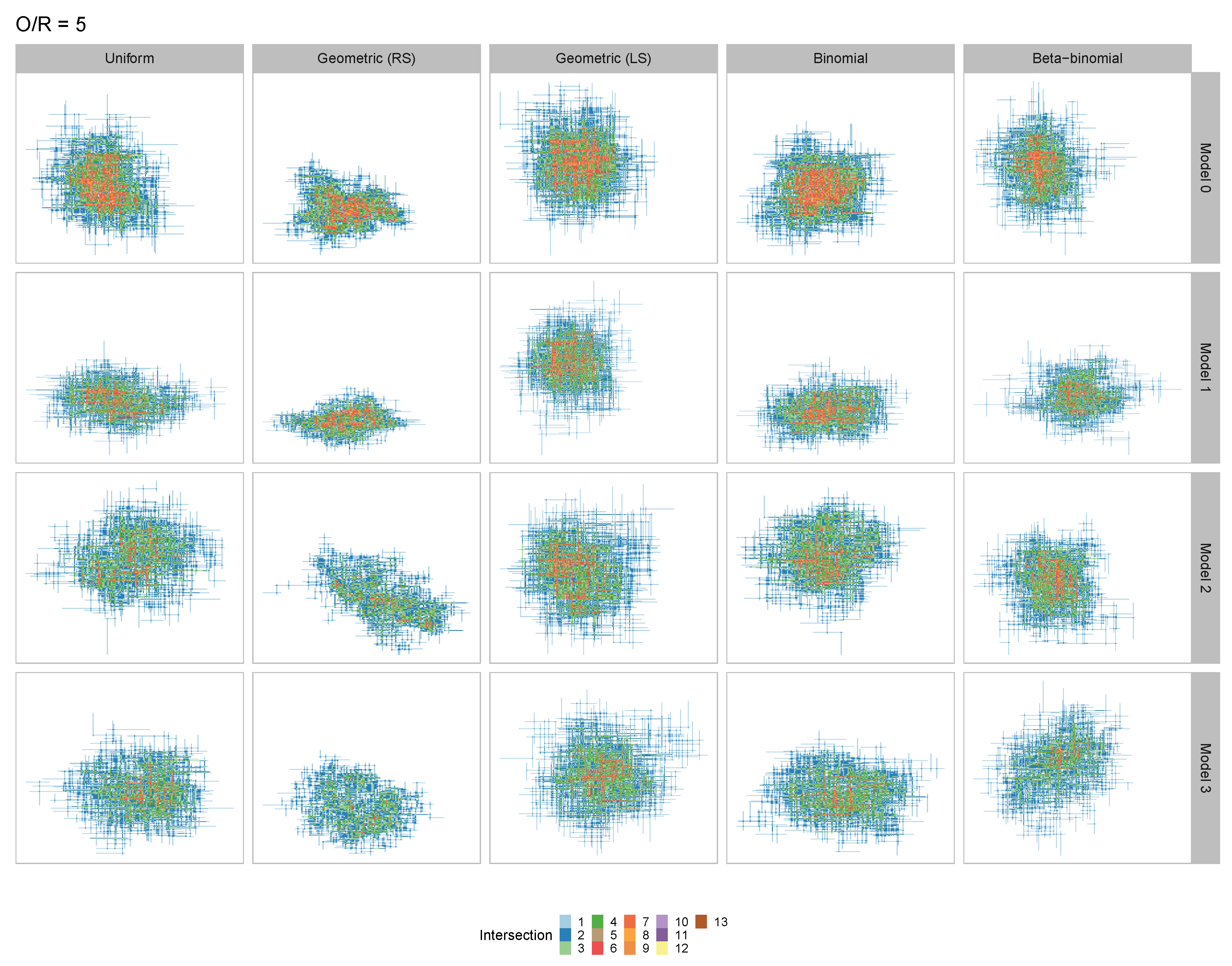
3.1. Coarse-Grained Computational Modeling of the DNA-Fibril Dynamical System
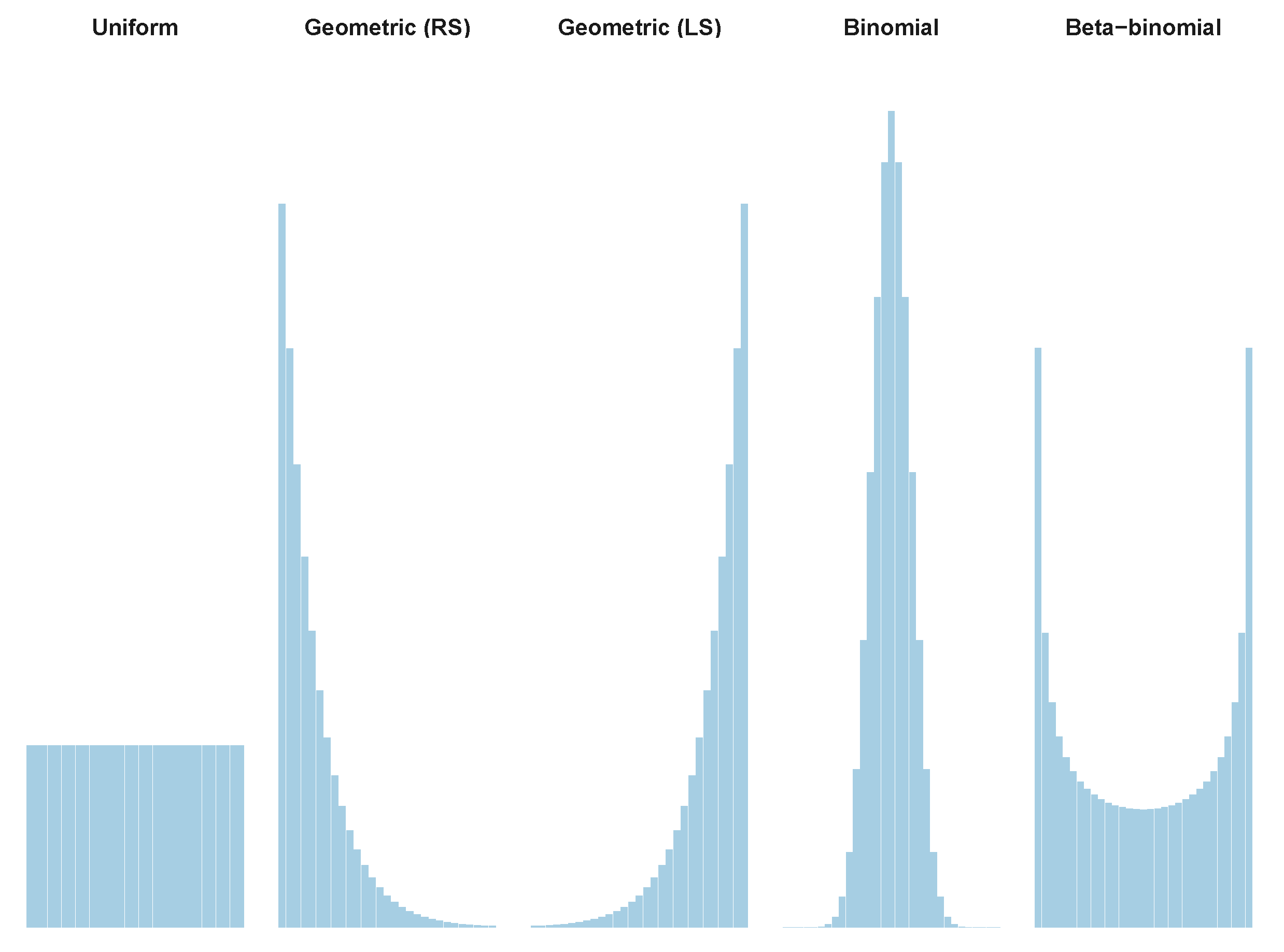
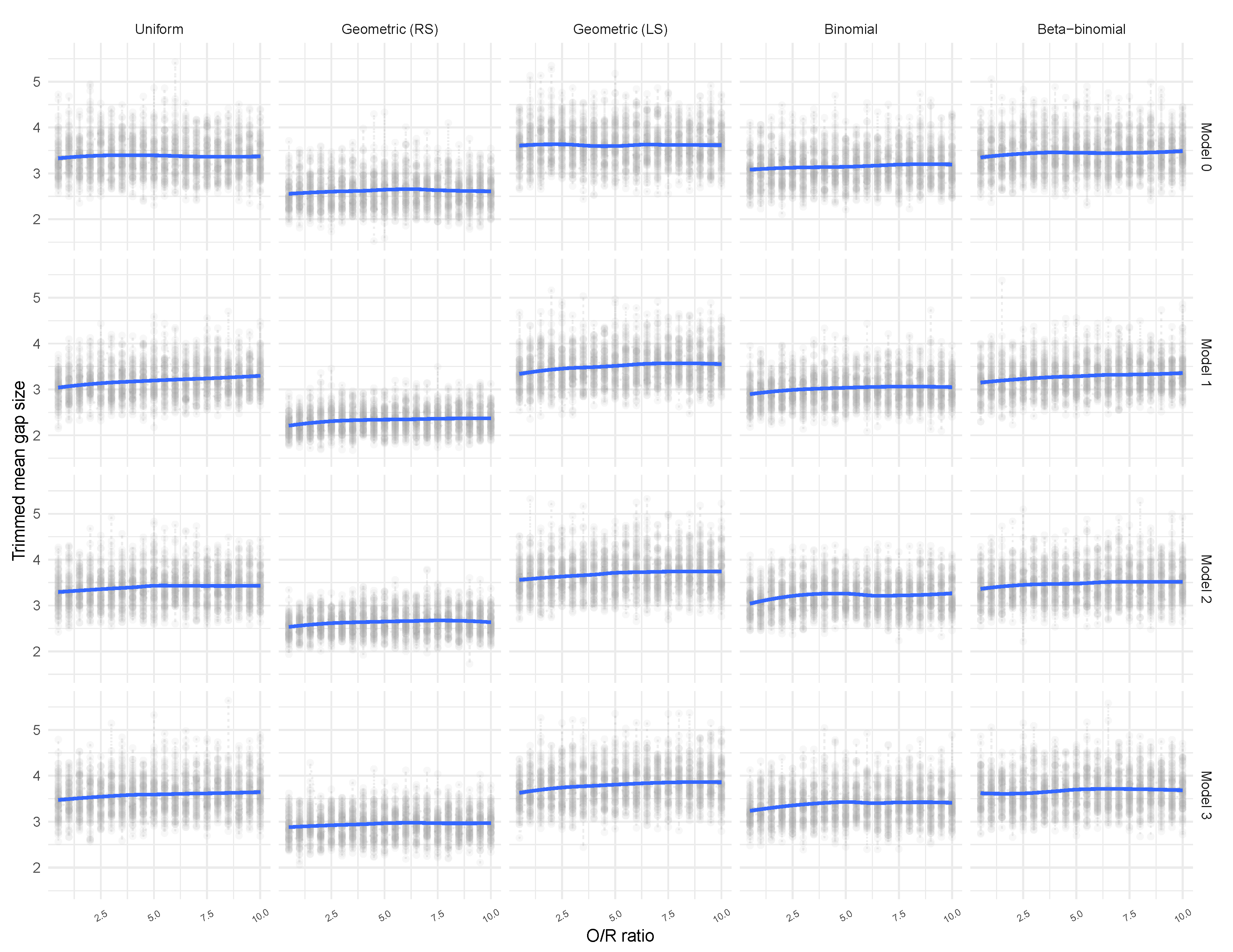
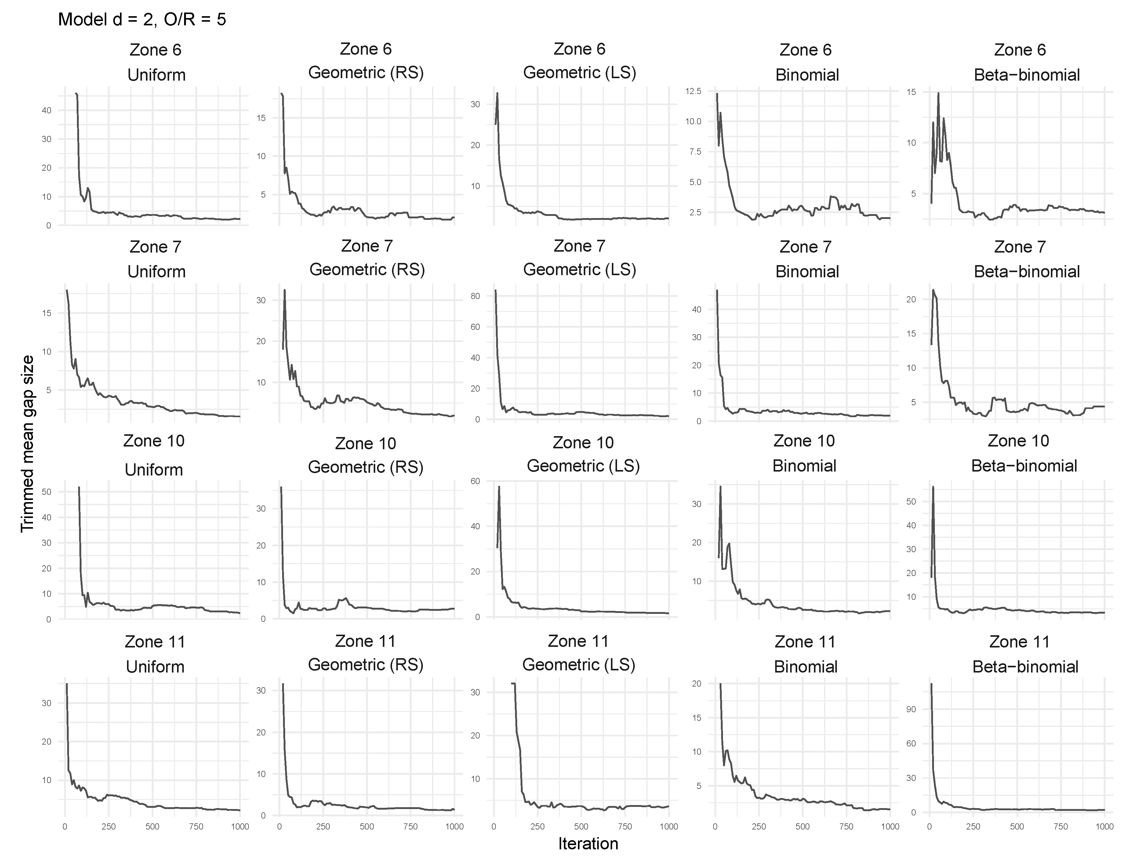
3.2. Tailored Stochastic Modeling of Assembly Formation and Dynamics
| zone 1 | zone 2 | zone 3 | zone 4 |
| zone 5 | zone 6 | zone 7 | zone 8 |
| zone 9 | zone 10 | zone 11 | zone 12 |
| zone 13 | zone 14 | zone 15 | zone 16 |
4. Discussion
Author Contributions
Funding
Institutional Review Board Statement
Informed Consent Statement
Acknowledgments
Conflicts of Interest
Appendix A
Appendix A.1. Table of Reference Distributions

| Distribution | Acronym | Parameters | |
|---|---|---|---|
| Beta | beta | ||
| Burr | burr | , | |
| Dagum | dagum1 | , | |
| Gumbel | gumbel | , | |
| Logistic | logis | , | |
| Log-Logistic | llogis | ||
| Gamma | gamma | ||
| Pareto 1 | pareto1 | , | |
| Weibull | weibull | ||
| Inverse Weibull | invweibull | ||
| Normal | norm | , | |
| Log-Normal | lnorm | ||
| Generalized Extreme Value | gev | ; , | |
| Nakagami | naka | , , | |
| Rayleigh | rayleigh | , |
Appendix A.2. Table of Top Ranked Fitted Distributions
| Distribution | Zones | Rank_Dist_1 | Rank_Dist_2 | Rank_Dist_3 | Rank_Dist_4 | Rank_Dist_5 |
|---|---|---|---|---|---|---|
| Uniform | z6 | gumbel | gev | lnorm | beta | dagum1 |
| Uniform | z7 | dagum1 | burr | gumbel | llogis | lnorm |
| Uniform | z10 | burr | dagum1 | gev | gumbel | llogis |
| Uniform | z11 | gumbel | dagum1 | lnorm | burr | llogis |
| Uniform | all | gamma | lnorm | nakagami | burr | normal |
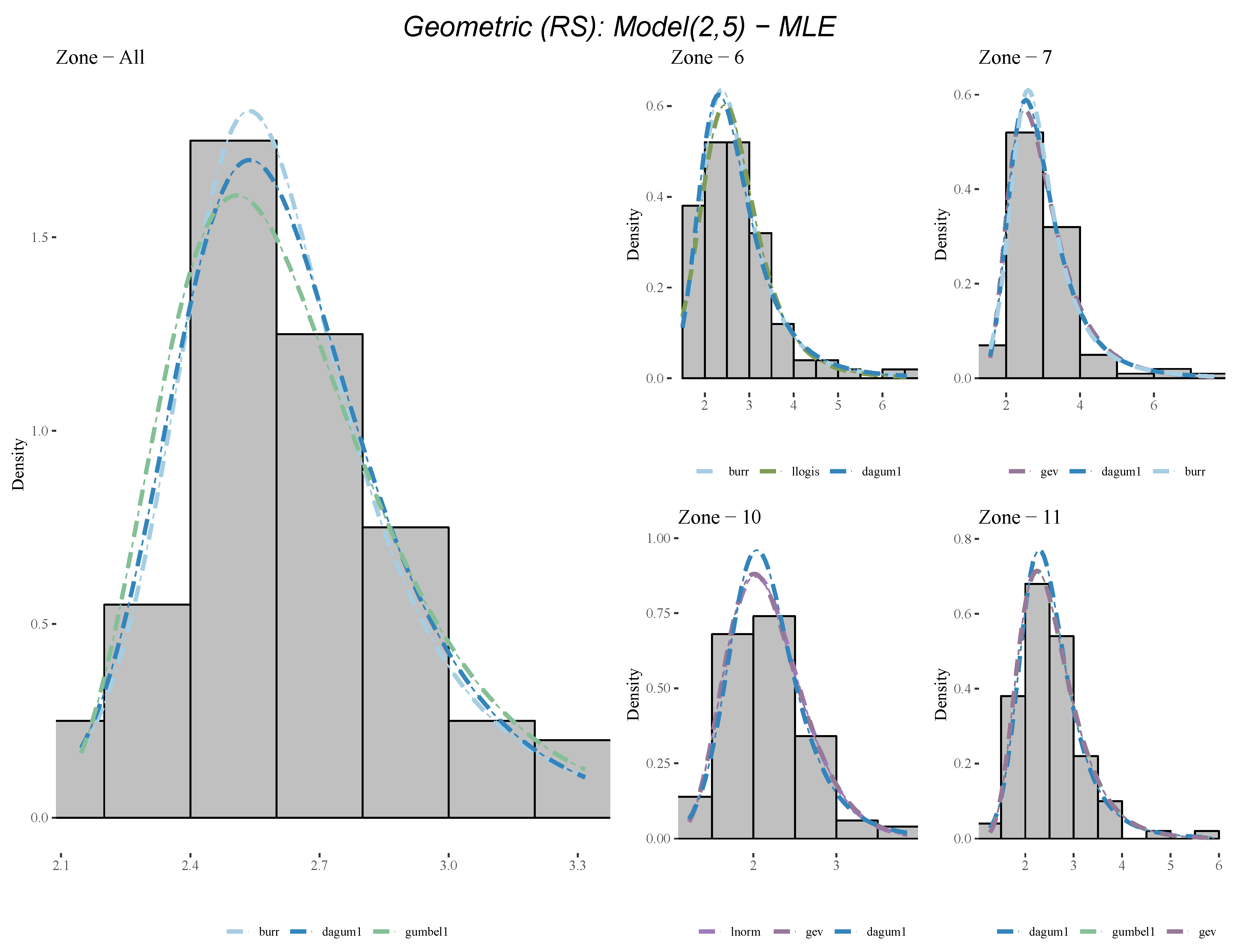
| Geometric (RS) | z6 | burr | llogis | dagum1 | gumbel | lnorm |
| Geometric (RS) | z7 | gev | dagum1 | burr | gumbel | llogis |
| Geometric (RS) | z10 | lnorm | gev | dagum1 | llogis | burr |
| Geometric (RS) | z11 | dagum1 | gumbel | gev | burr | llogis |
| Geometric (RS) | all | burr | dagum1 | gumbel | llogis | invweibull |
| Geometric (LS) | z6 | gev | gumbel | dagum1 | lnorm | burr |
| Geometric (LS) | z7 | gev | lnorm | gumbel | gamma | dagum1 |
| Geometric (LS) | z10 | burr | gumbel | dagum1 | llogis | lnorm |
| Geometric (LS) | z11 | llogis | burr | dagum1 | lnorm | gamma |
| Geometric (LS) | all | gamma | lnorm | nakagami | normal | burr |
| Binomial | z6 | dagum1 | burr | llogis | gumbel | gev |
| Binomial | z7 | gumbel | gev | lnorm | dagum1 | burr |
| Binomial | z10 | gumbel | gev | lnorm | dagum1 | burr |
| Binomial | z11 | dagum1 | gumbel | lnorm | burr | llogis |
| Binomial | all | gumbel | dagum1 | invweibull | burr | lnorm |
| Beta-binomial | z6 | gev | lnorm | gamma | dagum1 | llogis |
| Beta-binomial | z7 | burr | dagum1 | gev | invweibull | gumbel |
| Beta-binomial | z10 | burr | dagum1 | gumbel | llogis | lnorm |
| Beta-binomial | z11 | gev | lnorm | gumbel | dagum1 | llogis |
| Beta-binomial | all | gev | lnorm | burr | llogis | dagum1 |
References
- Ding, L.; Wei, Y.; Li, L.; Zhang, T.; Wang, H.; Xue, J.; Ding, L.X.; Wang, S.; Caro, J.; Gogotsi, Y. MXene molecular sieving membranes for highly efficient gas separation. Nat. Commun. 2018, 9, 155. [Google Scholar] [CrossRef]
- Xiong, G.; He, P.; Lyu, Z.; Chen, T.; Huang, B.; Chen, L.; Fisher, T.S. Bioinspired leaves-on-branchlet hybrid carbon nanostructure for supercapacitors. Nat. Commun. 2018, 9, 790. [Google Scholar] [CrossRef] [Green Version]
- Zhang, K.; Lin, S.; Feng, Q.; Dong, C.; Yang, Y.; Li, G.; Bian, L. Nanocomposite hydrogels stabilized by self-assembled multivalent bisphosphonate-magnesium nanoparticles mediate sustained release of magnesium ion and promote in-situ bone regeneration. Acta Biomater. 2017, 64, 389–400. [Google Scholar] [CrossRef]
- Jang, Y.; Choi, W.T.; Johnson, C.T.; García, A.J.; Singh, P.M.; Breedveld, V.; Hess, D.W.; Champion, J.A. Inhibition of Bacterial Adhesion on Nanotextured Stainless Steel 316L by Electrochemical Etching. ACS Biomater. Sci. Eng. 2018, 4, 90–97. [Google Scholar] [CrossRef] [Green Version]
- Chen, W.T.; Zhu, A.Y.; Sanjeev, V.; Khorasaninejad, M.; Shi, Z.; Lee, E.; Capasso, F. A broadband achromatic metalens for focusing and imaging in the visible. Nat. Nanotechnol. 2018, 13, 220–226. Available online: https://www.nature.com/articles/s41565-017-0034-6 (accessed on 8 February 2021). [CrossRef] [PubMed] [Green Version]
- Park, J.H.; Rutledge, G.C. Ultrafine high performance polyethylene fibers. J. Mater. Sci. 2018, 53, 3049–3063. [Google Scholar] [CrossRef] [Green Version]
- Ware, C.S.; Smith-Palmer, T.; Peppou-Chapman, S.; Scarratt, L.R.; Humphries, E.M.; Balzer, D.; Neto, C. Marine Antifouling Behavior of Lubricant-Infused Nanowrinkled Polymeric Surfaces. ACS Appl. Mater. Interfaces 2018, 10, 4173–4182. [Google Scholar] [CrossRef]
- Snow, R.J.; Bhatkar, H.; Diaye, A.T.N.; Arenholz, E.; Idzerda, Y.U.; Snow, R.J.; Bhatkar, H.; Diaye, A.T.N.; Arenholz, E.; Idzerda, Y.U. Large moments in bcc FexCoyMnz ternary alloy thin films. Appl. Phys. Lett. 2018, 112, 1–5. [Google Scholar] [CrossRef]
- Picker, A.; Nicoleau, L.; Burghard, Z.; Bill, J.; Zlotnikov, I.; Labbez, C.; Nonat, A.; Cölfen, H. Mesocrystalline calcium silicate hydrate: A bioinspired route toward elastic concrete materials. Sci. Adv. 2017, 3. Available online: https://advances.sciencemag.org/content/3/11/e1701216 (accessed on 8 February 2021). [CrossRef] [PubMed] [Green Version]
- Yuan, C.; Wu, Q.; Li, Q.; Duan, Q.; Li, Y.; Wang, H.G. Nanoengineered Ultralight Organic Cathode Based on Aromatic Carbonyl Compound/Graphene Aerogel for Green Lithium and Sodium Ion Batteries. ACS Sustain. Chem. Eng. 2018, 6, 8392–8399. [Google Scholar] [CrossRef]
- Kuzyk, A.; Laitinen, K.T.; Törmä, P. DNA origami as a nanoscale template for protein assembly. Nanotechnology 2009, 20, 235305:1–235305:5. [Google Scholar] [CrossRef]
- Kuzyk, A.; Schreiber, R.; Fan, Z.; Pardatscher, G.; Roller, E.M.; Högele, A.; Simmel, F.C.; Govorov, A.O.; Liedl, T. DNA-based self-assembly of chiral plasmonic nanostructures with tailored optical response. Nature 2012, 483, 311–314. Available online: https://www.nature.com/articles/nature10889 (accessed on 8 February 2021). [CrossRef] [Green Version]
- Tikhomirov, G.; Petersen, P.; Qian, L. Fractal assembly of micrometre-scale DNA origami arrays with arbitrary patterns. Nature 2017, 552, 67–71. Available online: https://www.nature.com/articles/nature24655 (accessed on 8 February 2021). [CrossRef] [PubMed] [Green Version]
- Benson, E.; Mohammed, A.; Gardell, J.; Masich, S.; Czeizler, E.; Orponen, P.; Högberg, B. DNA rendering of polyhedral meshes at the nanoscale. Nature 2015, 523, 441–444. Available online: https://www.nature.com/articles/nature14586 (accessed on 8 February 2021). [CrossRef] [PubMed] [Green Version]
- Zhang, X.; Ding, X.; Zou, J.; Gu, H. A proximity-based programmable DNA nanoscale assembly line. Methods Mol. Biol. 2017, 1500, 257–268. Available online: https://pubmed.ncbi.nlm.nih.gov/27813014/ (accessed on 8 February 2021).
- Lund, K.; Manzo, A.J.; Dabby, N.; Michelotti, N.; Johnson-Buck, A.; Nangreave, J.; Taylor, S.; Pei, R.; Stojanovic, M.N.; Walter, N.G.; et al. Molecular robots guided by prescriptive landscapes. Nature 2010, 465, 206–209. [Google Scholar] [CrossRef] [Green Version]
- Koh, L.D.; Cheng, Y.; Teng, C.P.; Khin, Y.W.; Loh, X.J.; Tee, S.Y.; Low, M.; Ye, E.; Yu, H.D.; Zhang, Y.W.; et al. Structures, mechanical properties and applications of silk fibroin materials. Prog. Polym. Sci. 2015, 46, 86–110. [Google Scholar] [CrossRef]
- Charrier, E.E.; Janmey, P.A. Chapter Two—Mechanical Properties of Intermediate Filament Proteins. Methods Enzymol. 2016, 568, 35–57. [Google Scholar] [CrossRef] [Green Version]
- Pal, S.; Deng, Z.; Ding, B.; Yan, H.; Liu, Y. DNA-Origami-Directed Self-Assembly of Discrete Silver-Nanoparticle Architectures. Angew. Chem. Int. Ed. 2010, 49, 2700–2704. [Google Scholar] [CrossRef]
- Scharnweber, D.; Bierbaum, S.; Wolf-Brandstetter, C. Utilizing DNA for functionalization of biomaterial surfaces. FEBS Lett. 2018, 592, 2181–2196. [Google Scholar] [CrossRef] [Green Version]
- Alarcon, L.P.; Baena, Y.; Manzo, R.H. Interaction between DNA and Drugs Having Protonable Basic Groups: Characterization through Affinity Constants, Drug Release Kinetics, and Conformational Changes. Sci. Pharm. 2017, 85, 1. [Google Scholar] [CrossRef] [Green Version]
- Inoue, Y.; Fukushima, T.; Hayakawa, T.; Takeuchi, H.; Kaminishi, H.; Miyazaki, K.; Okahata, Y. Antibacterial characteristics of newly developed amphiphilic lipids and DNA–lipid complexes against bacteria. J. Biomed. Mater. Res. Part A 2003, 65A, 203–208. [Google Scholar] [CrossRef]
- Maune, H.T.; Han, S.P.; Barish, R.D.; Bockrath, M.; Iii, W.A.; Rothemund, P.W.; Winfree, E. Self-assembly of carbon nanotubes into two-dimensional geometries using DNA origami templates. Nat. Nanotechnol. 2010, 5, 61–66. [Google Scholar] [CrossRef] [Green Version]
- Eskelinen, A.P.; Kuzyk, A.; Kaltiaisenaho, T.K.; Timmermans, M.Y.; Nasibulin, A.G.; Kauppinen, E.I.; Törmä, P. Assembly of single-walled carbon nanotubes on DNA-origami templates through streptavidin-biotin interaction. Small 2011, 7, 746–750. [Google Scholar] [CrossRef]
- Amărioarei, A.; Barad, G.; Czeizler, E.; Dobre, A.M.; Iţcuş, C.; Mitrana, V.; Păun, A.; Păun, M.; Spencer, F.; Trandafir, R.; et al. DNA-Guided Assembly of Nanocellulose Meshes. In Theory and Practice of Natural Computing; Fagan, D., Martín-Vide, C., O’Neill, M., Vega-Rodríguez, M.A., Eds.; Springer International Publishing: Cham, Switzerland, 2018; pp. 253–265. [Google Scholar]
- Faeder, J.R.; Blinov, M.L.; Goldstein, B.; Hlavacek, W.S. Rule-based modeling of biochemical networks. Complexity 2005, 10, 22–41. [Google Scholar] [CrossRef]
- Faeder, J.R.; Blinov, M.L.; Hlavacek, W.S. Rule-based modeling of biochemical systems with BioNetGen. In Methods in Molecular Biology; Humana Press: Totowa, NJ, USA, 2009; Volume 500, pp. 113–167. Available online: https://pubmed.ncbi.nlm.nih.gov/19399430/ (accessed on 8 February 2021).
- Rothemund, P.W. Folding DNA to create nanoscale shapes and patterns. Nature 2006, 440, 297–302. Available online: https://www.nature.com/articles/nature04586 (accessed on 8 February 2021). [CrossRef] [PubMed] [Green Version]
- Woo, S.; Rothemund, P.W.K. Programmable molecular recognition based on the geometry of DNA nanostructures. Nat. Chem. 2011, 3, 620–627. [Google Scholar] [CrossRef]
- Sneddon, M.W.; Faeder, J.R.; Emonet, T. Efficient modeling, simulation and coarse-graining of biological complexity with NFsim. Nat. Methods 2011, 8, 177–183. [Google Scholar] [CrossRef] [PubMed]
- Smith, A.M. Rulebender: Integrated Modeling, Simulation and Visualization for Rule-Based Intracellular Biochemistry. BMC J. Bioinform. 2012, 13, 1–39. [Google Scholar] [CrossRef] [PubMed] [Green Version]
- Hogg, R.V.; McKean, J.; Craig, A.T. Introduction to Mathematical Statistics, 7th ed.; Pearson: Boston, MA, USA, 2012. [Google Scholar]
- D’Agostino, R.; Stephens, M. Goodness-of-Fit Techniques, 1st ed.; Marcel Dekker, Inc.: New York, NY, USA, 1986. [Google Scholar]
- Luceno, A. Fitting the Generalized Pareto Distribution to Data Using Maximum Goodness-of-fit Estimators. Comput. Stat. Data Anal. 2006, 51, 904–917. [Google Scholar] [CrossRef]
- Delignette-Muller, M.; Pouillot, R.; Denis, J.; Dutang, C. Fitdistrplus: An R Package for Fitting Distributions. J. Stat. Softw. 2015, 64, 1–34. [Google Scholar] [CrossRef] [Green Version]
- Dutang, C.; Goulet, V.; Pigeon, M. Actuar: An R Package for Actuarial Science. J. Stat. Softw. 2008, 25, 1–37. [Google Scholar]
- Yee, T. Vector Generalized Linear and Additive Models: With an Implementation in R; Springer: New York, NY, USA, 2015. [Google Scholar]
- Qi, Y.; Wang, H.; Wei, K.; Yang, Y.; Zheng, R.Y.; Kim, I.S.; Zhang, K.Q. A Review of Structure Construction of Silk Fibroin Biomaterials from Single Structures to Multi-Level Structures. Int. J. Mol. Sci. 2017, 18, 237. [Google Scholar] [CrossRef]


| Distribution | z6 | z7 | z10 | z11 | All |
|---|---|---|---|---|---|
| Uniform | 3.2675 | 3.4093 | 3.2805 | 3.5288 | 3.5151 |
| Geometric (RS) | 2.7425 | 3.0276 | 2.1810 | 2.5424 | 2.6354 |
| Geometric (LS) | 3.5283 | 3.3386 | 3.4199 | 3.3275 | 3.6453 |
| Binomial | 3.1354 | 2.9235 | 3.1980 | 3.0020 | 3.2363 |
| Beta-binomial | 3.3983 | 3.4945 | 3.5101 | 3.4127 | 3.5035 |
| Distribution | Model | O/R Ratio | Fitted Distribution |
|---|---|---|---|
| Beta-binomial | 2 | 5 | gev |
| Binomial | 2 | 5 | gumbel |
| Geometric (LS) | 2 | 5 | lnorm |
| Geometric (RS) | 2 | 5 | dagum1 |
| Uniform | 2 | 5 | gumbel |
Publisher’s Note: MDPI stays neutral with regard to jurisdictional claims in published maps and institutional affiliations. |
© 2021 by the authors. Licensee MDPI, Basel, Switzerland. This article is an open access article distributed under the terms and conditions of the Creative Commons Attribution (CC BY) license (http://creativecommons.org/licenses/by/4.0/).
Share and Cite
Amărioarei, A.; Spencer, F.; Barad, G.; Gheorghe, A.-M.; Iţcuş, C.; Tuşa, I.; Prelipcean, A.-M.; Păun, A.; Păun, M.; Rodriguez-Paton, A.; et al. DNA-Guided Assembly for Fibril Proteins. Mathematics 2021, 9, 404. https://doi.org/10.3390/math9040404
Amărioarei A, Spencer F, Barad G, Gheorghe A-M, Iţcuş C, Tuşa I, Prelipcean A-M, Păun A, Păun M, Rodriguez-Paton A, et al. DNA-Guided Assembly for Fibril Proteins. Mathematics. 2021; 9(4):404. https://doi.org/10.3390/math9040404
Chicago/Turabian StyleAmărioarei, Alexandru, Frankie Spencer, Gefry Barad, Ana-Maria Gheorghe, Corina Iţcuş, Iris Tuşa, Ana-Maria Prelipcean, Andrei Păun, Mihaela Păun, Alfonso Rodriguez-Paton, and et al. 2021. "DNA-Guided Assembly for Fibril Proteins" Mathematics 9, no. 4: 404. https://doi.org/10.3390/math9040404