
Identification of Hotspot Segments with a Risk of Heavy-Vehicle Accidents Based on Spatial Analysis at Controlled-Access Highway

 ,
,  ,
,
Abstract
:1. Introduction
2. Study Area and Data Collection
2.1. Study Area
2.2. Road Network and Accident Data
3. Research Methodology
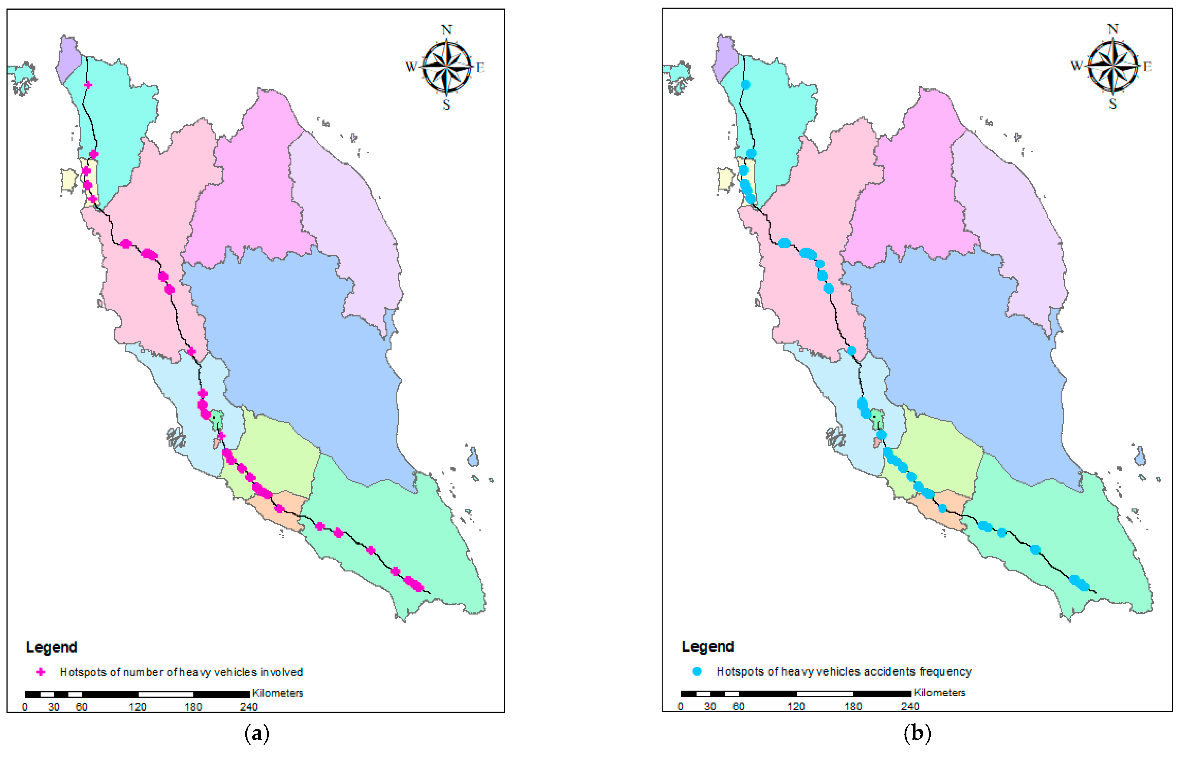
3.1. Spatial Location Displaying
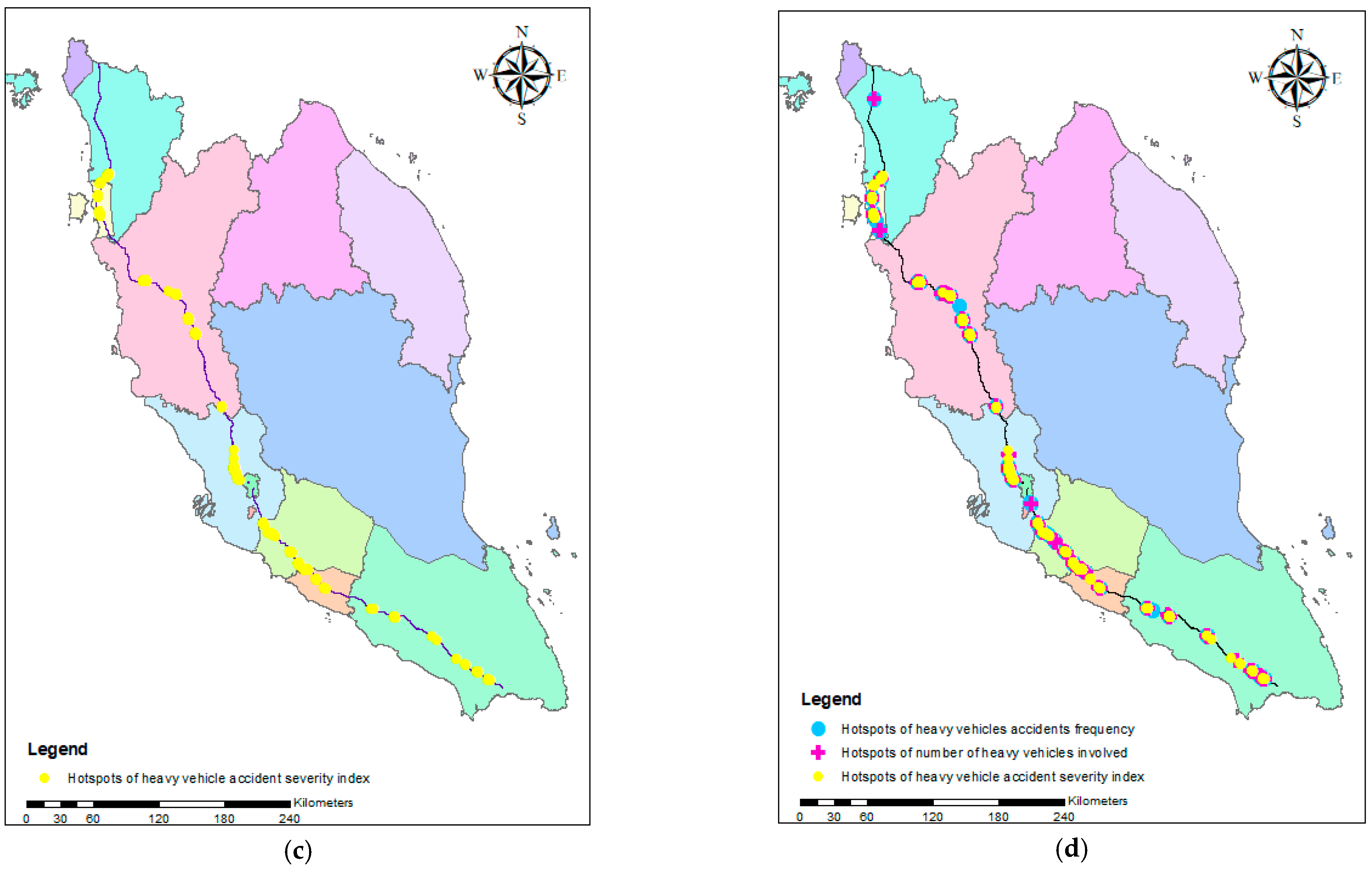
3.2. Severity Index
3.3. Spatial Autocorrelation
3.4. Hotspot Analysis Getis–Ord Gi*
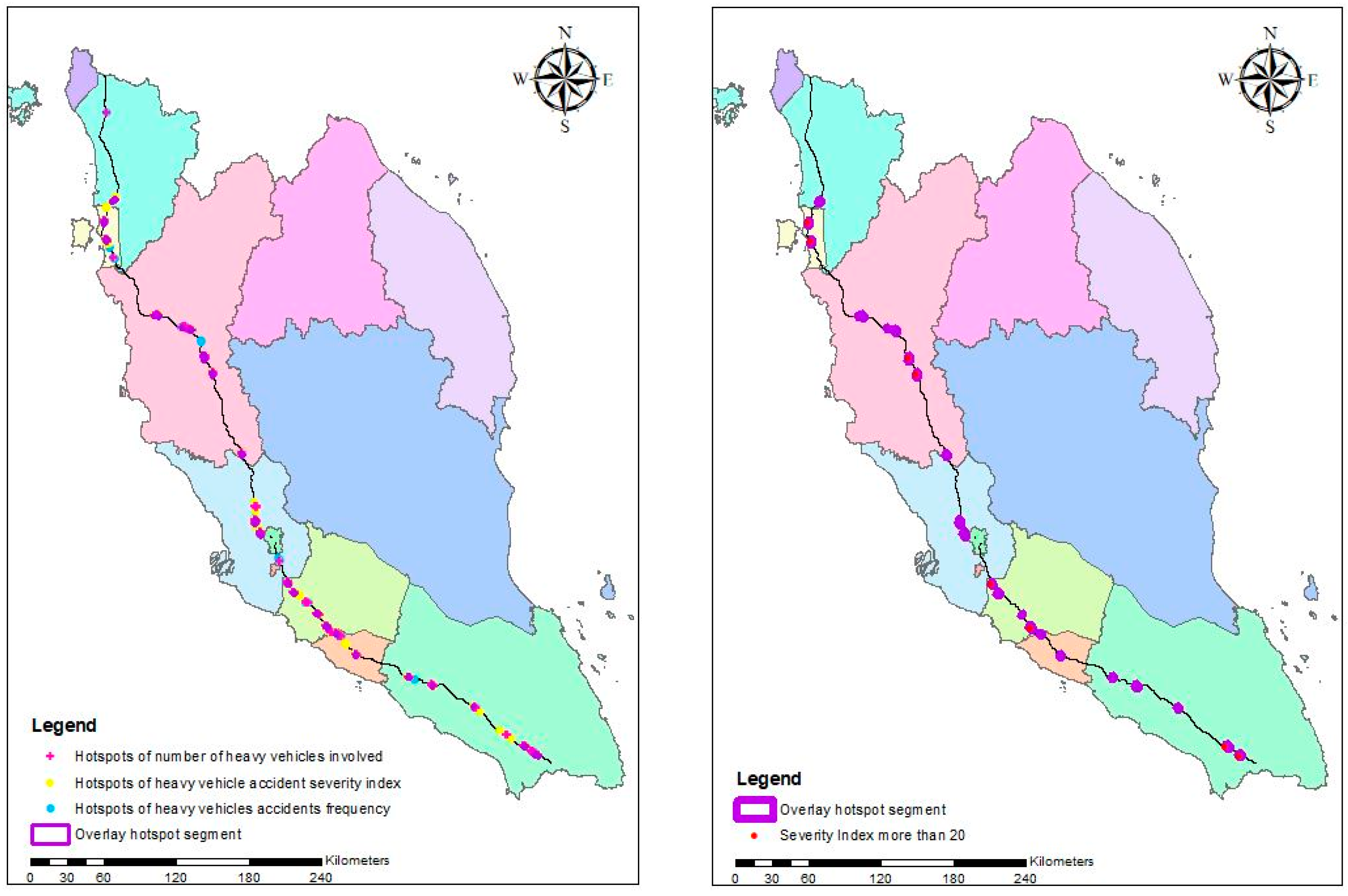
3.5. Ranking the Heavy Vehicle Risk Segment
4. Result and Discussion
5. Conclusions
6. Limitation of the Study and Further Direction of the Study
Author Contributions
Funding
Institutional Review Board Statement
Informed Consent Statement
Data Availability Statement
Acknowledgments
Conflicts of Interest
Abbreviations
| ArcGIS | Geographic information system application |
| CL | Confidence level |
| DEM | Cell-based digital elevation model |
| E1 | Northern routes of the NSE |
| E2 | Southern routes of the NSE |
| GIS | Geographic information system |
| HGV | Heavy goods vehicle |
| HVRS | Heavy vehicle risk segment |
| KDE | Kernel density estimation |
| KM | Kilometer Marker |
| LISA | Local indicators of spatial association |
| MHA | Malaysian Highway Authority |
| MIROS | Malaysian Institute of Road Safety Research |
| NHTSA | United States National Highway Traffic Safety Administration |
| NSE | North–South Expressway |
| ROCA | ROad Curvature Analyst |
| RSO | Rectified skewed orthomorphic |
| UAE | United Arab Emirates |
| WGS84 | World Geodetic System 1984 |
| CR | Crash rate |
| C | Total number of crashes in the study period |
| ADT | Average daily traffic volume |
| n | Number of years of data |
| L | Segment length in km |
| Hvcf | Total heavy vehicle crashes at the hotspot segment in the study period |
| Heavy vehicle volume in the study period at the hotspot segment | |
| Lh | Length of the heavy vehicle hotspots segment |
| ωij | Spatial weight |
| zi | Deviation of an attribute for feature from its mean |
| So | Aggregate of all spatial weights |
| Gi* | Getis–Ord Gi* z-score value |
| xj | Attribute value feature j |
| d | Fixed band radius around segment i |
| Number of weighted points |
Appendix A

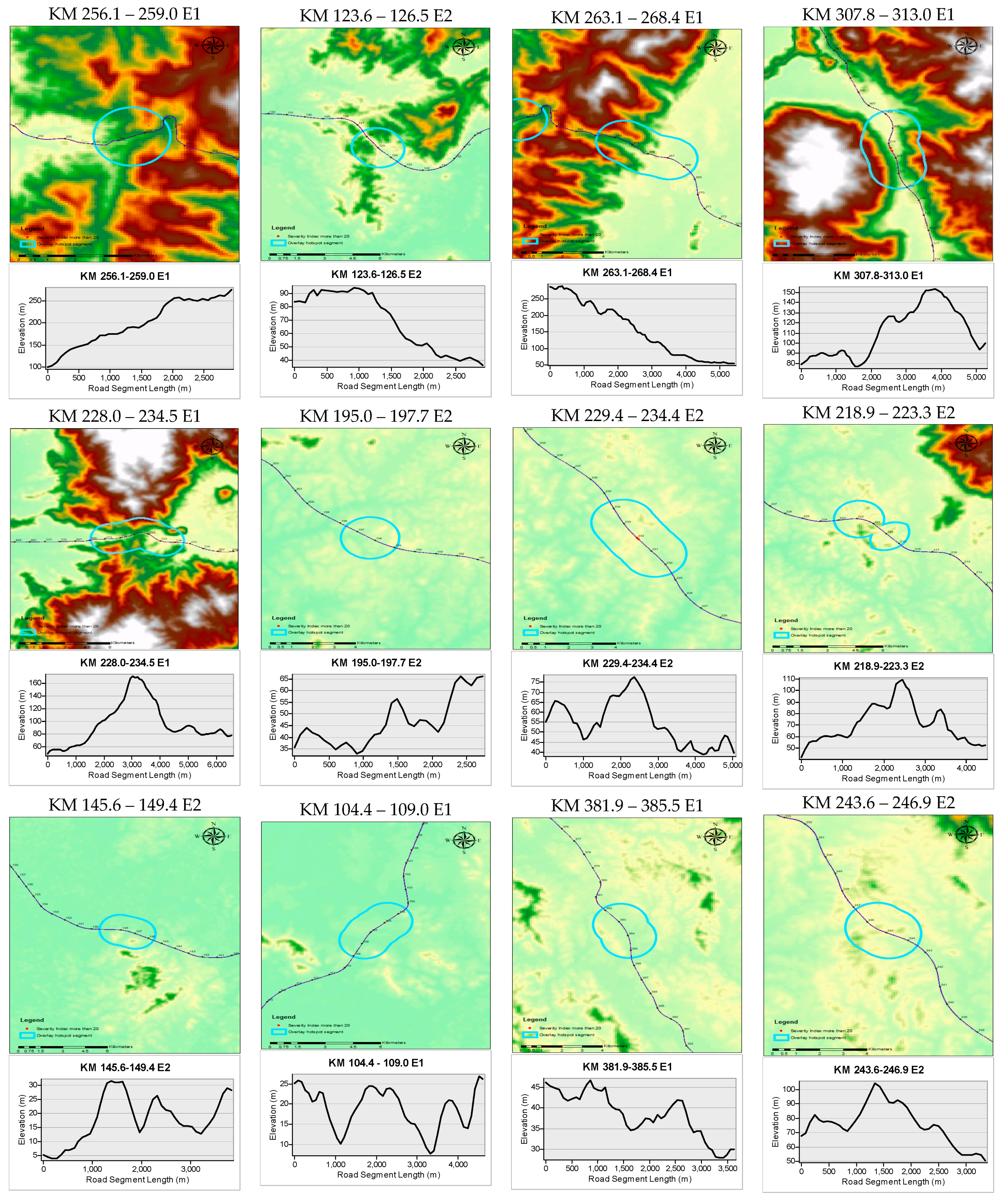
| KM | Length (km) | Elevation Gain | Elevation Loss | Average Slope | Max Slope | Number of Lanes | Curve Radius (m) | Rank | ||
|---|---|---|---|---|---|---|---|---|---|---|
| 256.1–259.0 E1 | 2.9 | 147 | 0 | 4.90% | 0.00% | 9.80% | 0.00% | 5 | 227–1798 | 1 |
| 123.6–126.5 E2 | 2.9 | 45.1 | −99 | 3.70% | −5.00% | 13.30% | −17.00% | 4 | 1422–2771 | 2 |
| 263.1–268.4 E1 | 5.4 | 4.5 | −208 | 0.90% | −3.90% | 9.70% | −14.40% | 5 | 215–2839 | 3 |
| 307.8–313.0 E1 | 5.2 | 115 | −89.6 | 3.80% | −3.20% | 30.50% | −26.70% | 4 | 995–1947 | 4 |
| 228.0–234.5 E1 | 6.5 | 168 | −138 | 4.10% | −5.10% | 17.50% | −17.10% | 4 | 892–2801 | 5 |
| 195.0–197.7 E2 | 2.7 | 33.5 | −10.7 | 1.70% | −1.20% | 14.90% | −15.00% | 6 | – | 6 |
| 229.4–234.4 E2 | 5.0 | 71.7 | −89.2 | 3.20% | −2.90% | 13.40% | −8.60% | 6 | – | 7 |
| 218.9–223.3 E2 | 4.4 | 57.4 | −52.9 | 2.20% | −2.30% | 13.20% | −9.50% | 6 | 1520 | 8 |
| 145.6–149.4 E2 | 3.8 | 65.2 | −40.9 | 2.80% | −2.50% | 7.60% | −9.60% | 4 | 2455 | 9 |
| 104.4–109.0 E1 | 4.6 | 55.2 | −51.3 | 1.90% | −2.20% | 29.60% | −31.70% | 4 | 683–2022 | 10 |
| 381.9–385.5 E1 | 3.6 | 25.4 | −39.7 | 7.70% | −6.20% | 1.60% | −1.80% | 6 | 2106–2998 | 11 |
| 243.6–246.9 E2 | 3.3 | 58.3 | −73 | 4.00% | −3.70% | 12.60% | −13.80% | 6 | 1097–2684 | 12 |
| 292.0–297.1 E1 | 5.1 | 37.2 | −71.9 | 2.10% | −1.90% | 14.40% | −18.70% | 4 | 1504–2653 | 13 |
| 81.0–83.01 E2 | 2.0 | 25.8 | −17.2 | 1.80% | −2.40% | 7.50% | −6.00% | 4 | – | 14 |
| 271.0–275.5 E2 | 4.5 | 37.4 | −40.8 | 1.50% | −1.30% | 4.80% | −4.20% | 6 | 2478 | 15 |
| 25.5–30.61 E2 | 5.1 | 76 | −35.7 | 2.20% | −1.60% | 18.50% | −13.90% | 4 | 2013 | 16 |
| 125.7–131.0 E1 | 5.3 | 34.2 | −34.7 | 1.10% | −1.10% | 14.70% | −28.50% | 4 | 1674–2869 | 17 |
| 143.0–148.3 E1 | 5.3 | 28.6 | −29 | 0.80% | −1.00% | 11.90% | −19.00% | 4 | 1074–2947 | 18 |
| 280.9–285.5 E2 | 4.7 | 53.4 | −57.5 | 2.30% | 2.10% | 42.30% | −40.70% | 6 | 659–2789 | 19 |
| 12.6–17.61 E2 | 5.0 | 47 | −76.7 | 2.20% | −2.40% | 15.60% | −19.20% | 4 | – | 20 |
| 443.0–449.4 E1 | 6.4 | 79.4 | −55.2 | 1.90% | −2.00% | 25.80% | −29.10% | 8 | 598–2226 | 21 |
| 454.3–458.9 E1 | 4.6 | 82 | −44.9 | 2.60% | −2.90% | 26.10% | 27.60% | 8 | 244–1108 | 22 |
References
- Moridpour, S.; Mazloumi, E.; Mesbah, M. Impact of heavy vehicles on surrounding traffic characteristics. J. Adv. Transp. 2014, 49, 535–552. [Google Scholar] [CrossRef]
- Darus, N.S.; Borhan, M.N.; Ishak, S.Z.; Ismail, R.; Razali, S.F.M. Pattern of child pedestrian collisions and injuries in Malaysia. J. Teknol. 2018, 80, 23–31. [Google Scholar] [CrossRef] [Green Version]
- Dissanayake, S.; Bezwada, N. Characteristics and Contributory Causes Related to Large Truck Crashes (Phase I)—Fatal Crashes (Phase I); Kansas State University: Manhattan, KS, USA, 2010. [Google Scholar]
- National Highway Traffic Safety Administration (NHTSA). Traffic Safety Facts (2017 Data). Available online: https://crashstats.nhtsa.dot.gov/Api/Public/ViewPublication/812663 (accessed on 17 June 2020).
- Federal Motor Carier Safety Administration (FMCSA). Large Truck and Bus Crash Facts 2017. Available online: https://www.fmcsa.dot.gov/safety/data-and-statistics/large-truck-and-bus-crash-facts (accessed on 29 January 2021).
- Mooren, L.; Grzebieta, R.; Williamson, A.; Olivier, J.; Friswell, R. Safety management for heavy vehicle transport: A review of the literature. Saf. Sci. 2014, 62, 79–89. [Google Scholar] [CrossRef]
- Evgenikos, P.; Yannis, G.; Folla, K.; Bauer, R.; Machata, K.; Brandstaetter, C. Characteristics and causes of heavy goods vehicles and buses accidents in Europe. Transp. Res. Proc. 2016, 14, 2158–2167. [Google Scholar] [CrossRef] [Green Version]
- Hassan, H.M.; Albusaeedi, N.M.; Garib, A.M.; Al-Harthei, H.A. Exploring the nature and severity of heavy truck crashes in Abu Dhabi, United Arab Emirates. Transp. Res. Rec. 2015, 2517. [Google Scholar] [CrossRef]
- Björnstig, U.; Björnstig, J.; Eriksson, A. Passenger car collision fatalities—with special emphasis on collisions with heavy vehicles. Accid. Anal. Prev. 2008, 40, 158–166. [Google Scholar] [CrossRef]
- Pai, C.W.; Saleh, W. An analysis of motorcyclist injury severity under various traffic control measures at three-legged junctions in the UK. Saf. Sci. 2007, 45, 832–847. [Google Scholar] [CrossRef]
- Ministry of Transport Malaysia (MOT). Transport Statistic Malaysia. Available online: http://www.mot.gov.my/my/sumber-maklumat/statistik-tahunan-pengangkutan (accessed on 17 June 2020).
- Ibrahim, A.N.H.; Borhan, M.N.; Yunin, N.A.M. Getting young drivers to buckle up: Exploring the factors influencing seat belt use by young drivers in Malaysia. Sustainability 2021, 13, 162. [Google Scholar] [CrossRef]
- Road Safety Department Malaysia. Buku Statistik Kemalangan Jalan Raya Tahun 2018. Available online: http://jkjr.gov.my/ms/muat-turun-swasta/funcstartdown/139/lang,ms-my/ (accessed on 17 June 2020).
- Borhan, M.N.; Ibrahim, A.N.H.; Aziz, A.; Yazid, M.R.M. The relationship between the demographic, personal, and social factors of Malaysian motorcyclists and risk taking behavior at signalized intersections. Accid. Anal. Prev. 2018, 121, 94–100. [Google Scholar] [CrossRef]
- Hamidun, R.; Wah Hoong, A.; Roslan, A.; Shabadin, A.; Jamil, H. Characteristics of heavy goods vehicles (HGV) accidents in Malaysia. IOP Conf. Ser. Mater. Sci. Eng. 2019, 512, 29–31. [Google Scholar] [CrossRef]
- Haiqal, M.A.M.; Nuradira, W.E.W. Fatal Accidents Involving Truck in Malaysia (2014–2015). Universiti Teknologi MARA, n. d. Available online: https://www.arcgis.com/apps/Cascade/index.html?appid=b25fb43edde24a28a185782cee2eccbf (accessed on 17 June 2020).
- Khamis, N.K.; Deros, B.M.; Nuawi, M.Z.; Omar, R.B. Driving fatigue among long distance heavy vehicle drivers in Klang Valley, Malaysia. Appl. Mech. Mater. 2014, 663, 567–573. [Google Scholar] [CrossRef]
- Erdogan, S.; Yilmaz, I.; Baybura, T.; Gullu, M. Geographical information systems aided traffic accident analysis system case study: City of Afyonkarahisar. Accid. Anal. Prev. 2008, 40, 174–181. [Google Scholar] [CrossRef] [PubMed]
- Moons, E.; Brijs, T.; Wets, G. Identifying Hazardous Road Locations: Hot Spots versus Hot Zones. Lect. Notes Comput. Sci. 2009, 5730, 288–300. [Google Scholar] [CrossRef]
- Nie, K.; Wang, Z.; Du, Q.; Ren, F.; Tian, Q.A. Network-constrained integrated method for detecting spatial cluster and risk location of traffic crash: A case study from Wuhan, China. Sustainability 2015, 7, 2662–2677. [Google Scholar] [CrossRef] [Green Version]
- Harirforoush, H.; Bellalite, L. A new integrated GIS-based analysis to detect hotspots: A case study of the city of Sherbrooke. Accid. Anal. Prev. 2019, 130, 62–74. [Google Scholar] [CrossRef]
- Norhafizah, M.; Borhan, M.N.; Mat Yazid, M.; Hambali, M.; Rohan, A. Determining spatial patterns of road accidents at expressway by applying Getis-Ord Gi* spatial statistic. Int J Recent Technol Eng. 2019, 8, 345–350. [Google Scholar]
- Khorashadi, A.; Niemeier, D.; Shankar, V.; Mannering, F. Differences in rural and urban driver-injury severities in accidents involving large-trucks: An exploratory analysis. Accid. Anal. Prev. 2005, 37, 910–921. [Google Scholar] [CrossRef]
- Chen, F.; Chen, S. Injury severities of truck drivers in single- and multi-vehicle accidents on rural highways. Accid. Anal. Prev. 2011, 43, 1677–1688. [Google Scholar] [CrossRef]
- Chang, X.; Li, H.; Qin, L.; Rong, J.; Lu, Y.; Chen, X. Evaluation of cooperative systems on driver behavior in heavy fog condition based on a driving simulator. Accid. Anal. Prev. 2019, 128, 197–205. [Google Scholar] [CrossRef]
- Guerrieri, M.; Mauro, R.; Tollazzi, T. Turbo-roundabout: Case study of driver behavior and kinematic parameters of light and heavy vehicles. J. Transp. Eng. Part A Syst. 2019, 145. [Google Scholar] [CrossRef]
- Dong, C.; Clarke, D.B.; Richards, S.H.; Huang, B. Differences in passenger car and large truck involved crash frequencies at urban signalized intersections: An exploratory analysis. Accid. Anal. Prev. 2014, 62, 87–94. [Google Scholar] [CrossRef] [PubMed]
- Kang, N.; Nakamura, H. An analysis of characteristics of heavy vehicle behavior at roundabouts in Japan. Transp. Res. Proc 2017, 25, 1485–1493. [Google Scholar] [CrossRef]
- Hashim, W.; Arshad, A.K.; Mustaffa, M.; Kamaluddin, N.A. Heavy vehicles speed profiling on urban expressway: The case of federal highway. J. Teknol. 2016, 78, 19–23. [Google Scholar] [CrossRef] [Green Version]
- Chang, L.-Y.; Wang, H.-W. Analysis of traffic injury severity: An application of non parametric classification tree techniques. Accid. Anal. Prev. 2006, 38, 1019–1027. [Google Scholar] [CrossRef]
- Faghri, A.; Raman, N. A GIS-Based traffic accident information system. J. Adv. Transp. 1995, 29, 321–334. [Google Scholar] [CrossRef]
- Levine, N. Spatial statistics and GIS: Software tools to quantify spatial patterns. J. Am. Plann. Assoc. 1996, 62, 381–391. [Google Scholar] [CrossRef]
- Levine, N.; Kim, K.E. The location of motor vehicle crashes in Honolulu: A methodology for geocoding intersections. Comput. Env. Urban 1998, 22, 557–576. [Google Scholar] [CrossRef]
- Le, K.G.; Liu, P.; Lin, L.-T. Determining the road traffic accident hotspots using GIS based temporal-spatial statistical analytic techniques in Hanoi, Vietnam. Geo. Spat. Inf. Sci. 2019, 23, 153–164. [Google Scholar] [CrossRef] [Green Version]
- Briz-Redón, Á.; Martínez-Ruiz, F.; Montes, F. Identification of differential risk hotspots for collision and vehicle type in a directed linear network. Accid. Anal. Prev. 2019, 132, 105278. [Google Scholar] [CrossRef]
- Achu, A.L.; Aju, C.D.; Suresh, V.; Manoharan, T.P.; Reghunath, R. Spatio-temporal analysis of road accident incidents and delineation of hotspots using geospatial tools in Thrissur district, Kerala, India. Cart. Geogr. Inf. Sci. 2019, 69, 255–265. [Google Scholar] [CrossRef]
- Hasani, J.; Erfanpoor, S.; Rajabi, A.; Barzegar, A.; Khodadoost, M.; Afkar, M.; Hashemi Nazari, S.S. Spatial analysis of mortality rate of pedestrian accidents in Iran during 2012–2013. Traffic Inj. Prev. 2019, 20, 636–640. [Google Scholar] [CrossRef] [PubMed]
- Getis, A.; Ord, J.K. The analysis of spatial association by use of distance statistics. Geogr. Anal. 1992, 24, 189–206. [Google Scholar] [CrossRef]
- Zhang, Y. Hotspot Analysis of Highway Accident Spatial Pattern Based on Network Spatial Weights. Available online: https://ceprofs.civil.tamu.edu/folivera/TxAgGIS/Fall2010/Yanru%20Zhang.pdf (accessed on 29 January 2021).
- Anderson, T.K. Kernel density estimation and K-means clustering to profile road accident hotspots. Accid. Anal. Prev. 2009, 41, 359–364. [Google Scholar] [CrossRef]
- Manepalli, U.R.R.; Bham, G.H.; Kandada, S. Evaluation of Hotspots Identification Using Kernel Density Estimation (K) and Getis-Ord (Gi*) ON I-630; 3rd Int. Conf. Road Saf. Simul: Indianapolis, IN, USA, 2011; pp. 14–16. [Google Scholar]
- Flahaut, B.; Mouchart, M.; Martin, E.S.; Thomas, I. The local spatial autocorrelation and the kernel method for identifying black zones: A comparative approach. Accid. Anal. Prev. 2003, 35, 991–1004. [Google Scholar] [CrossRef]
- Steenberghen, T.; Dufays, T.; Thomas, I.; Flahaut, B. Intra-urban location and clustering of road accidents using GIS: A Belgian example. Int. J. Geogr. Inf. Sci. 2004, 18, 169–181. [Google Scholar] [CrossRef]
- Ouni, F.; Belloumi, M. Pattern of road traffic crash hot zones versus probable hot zones in Tunisia: A geospatial analysis. Accid. Anal. Prev. 2019, 128, 185–196. [Google Scholar] [CrossRef]
- Erdogan, S.; Ilçi, V.; Soysal, O.M.; Kormaz, A. A model suggestion for the determination of the traffic accident hotspots on the Turkish highway road network: A pilot study. Bol. Ciênc. Geod. 2015, 21, 169–188. [Google Scholar] [CrossRef]
- Kalinic, M.M.; Krisp, J. Kernel Density Estimation (KDE) vs. Hot-Spot Analysis—detecting criminal hot spots in the city of San Francisco. In Proceedings of the 21st AGILE International Conference on Geographic Information Science, Lund, Sweden, 12–15 June 2018. [Google Scholar]
- Satria, R.; Castro, M. GIS tools for analyzing accidents and road design: A review. Transp. Res. Proc. 2016, 18, 242–247. [Google Scholar] [CrossRef]
- Ulak, M.B.; Ozguven, E.E.; Vanli, O.A.; Horner, M.W. Exploring alternative spatial weights to detect crash hotspots. Comput. Env. Urban 2019, 78, 101398. [Google Scholar] [CrossRef]
- Anselin, L. Local indicators of spatial association-LISA. Geogr. Anal. 1995, 27, 93–115. [Google Scholar] [CrossRef]
- Public Works Department Malaysia (PWD). Arahan Teknik 8/86: A Guide on Geometric Design of Roads. Available online: https://www.academia.edu/34511665/Roads_Branch_Public_Works_Department_Malaysia_A_Guide_on_Geometric_Design_of_Roads (accessed on 17 June 2020).
- Malaysian Institute of Road Safety Research (MIROS). Guideline on Accident-Prone Area Identification for Automated Enforcement System (AES). Available online: https://miros.gov.my/xs/dl.php?filename=MCP115Guideline%20on%20APA%20for%20AES.pdf (accessed on 17 June 2020).
- Haining, R.P. Spatial autocorrelation. In International Encyclopedia of the Social & Behavioral Sciences; Pergamon Press: Oxford, UK, 2001; pp. 14763–14768. [Google Scholar]
- Mathur, M. Spatial autocorrelation analysis in plant population: An overview. J. Appl. Nat. Sci. 2015, 7, 501–513. [Google Scholar] [CrossRef] [Green Version]
- Boots, B.N.; Getis, A. Point Pattern Analysis; Sage Publication: Newburry Park, CA, USA, 1988. [Google Scholar]
- Rogerson, P.; Yamada, I. Statistical Detection and Surveillance of Geographic Clusters; Chapman and Hall/CRC: New York, NY, USA, 2009. [Google Scholar]
- Li, Y.; Liang, C. The analysis of spatial pattern and hotspots of aviation accident and ranking the potential risk airports based on GIS platform. J. Adv. Transp. 2018, 4027498. [Google Scholar] [CrossRef]
- Gundogdu, I.B. Applying linear analysis methods to GIS-supported procedures for preventing traffic accidents: Case study of Konya. Saf. Sci. 2010, 48, 763–769. [Google Scholar] [CrossRef]
- Kang, M.; Moudon, A.V.; Kim, H.; Boyle, L.N. Intersections and non-intersections: A protocol for identifying pedestrian crash risk locations in GIS. Int. J. Environ. Res. Public Health 2019, 16, 3565. [Google Scholar] [CrossRef] [PubMed] [Green Version]
- Rahman, N.H.; Rainis, R.; Noor, S.H.; Mohamad, S.M.S. The buffering analysis to identify common geographical factors within the vicinity of severe injury related to motor vehicle crash in Malaysia. World J. Emerg. Med. 2016, 7, 278–284. [Google Scholar] [CrossRef]
- Mestri, A.R.; Rathod, R.R.; Garg, D.R. Identification and removal of accident-prone locations using spatial data mining. In Applications of Geomatics in Civil Engineering; Springer: Singapore, 2019; pp. 383–394. [Google Scholar]
- Bíl, M.; Andrásík, R.; Sedoník, J.; Cícha, V. ROCA—An ArcGIS toolbox for road alignment identification and horizontal curve radii computation. PLoS ONE 2018, 13, e0208407. [Google Scholar] [CrossRef] [Green Version]
- Cerezoa, V.; Conche, F. Risk assessment in ramps for heavy vehicles—A French study. Accid. Anal. Prev. 2016, 91, 183–189. [Google Scholar] [CrossRef] [Green Version]
- Fu, R.; Guo, Y.; Yuan, W.; Feng, H.; Ma, Y. The correlation between gradients of descending roads and accident rates. Saf. Sci. 2011, 49, 416–423. [Google Scholar] [CrossRef]
- Rusli, R.B.; Mazharul, H.; Mark, K.; Voon, S.W. A comparison of road traffic crashes along mountainous and non-mountainous roads in Sabah, Malaysia. In Proceedings of the Australasian Road Safety Conference (ARSC2015), Goldcoast, Australia, 27 October 2015; pp. 1–12. [Google Scholar]


| Spatial Autocorrelation | Distance Threshold (m) | Moran’s I | Z-Score | p-Value | Spatial Autocorrelation | Null Hypothesis of Randomness |
|---|---|---|---|---|---|---|
| Frequency of heavy vehicle accident cases | 1355 | 0.0506 | 9.2754 | 0.00000 | Clustered | Rejected |
| Number of heavy vehicles | 1355 | 0.0623 | 11.2995 | 0.00000 | Clustered | Rejected |
| Severity index | 1355 | 0.0643 | 11.5154 | 0.00000 | Clustered | Rejected |
| Location of HVRS | Length (km) | Total Accidents Cases | Number of Heavy Vehicle Involved in Accident | Fatal | Severe Injury | Slight Injury | Property Damage | Severity Index | Exposure (Heavy Vehicle Kilometers of Travel) | Crash Rate per Million Heavy Vehicles | Rank |
|---|---|---|---|---|---|---|---|---|---|---|---|
| KM 104.4–109.0 E1 | 4.6 | 57 | 63 | 10 | 4 | 10 | 33 | 129 | 2,926,350 | 19.5 | 10 |
| KM 125.7–131.0 E1 | 5.3 | 58 | 62 | 2 | 9 | 10 | 37 | 105 | 4,897,491 | 11.8 | 17 |
| KM 143.0–148.3 E1 | 5.3 | 91 | 100 | 5 | 11 | 11 | 64 | 160 | 10,576,838 | 8.6 | 18 |
| KM 228.0–234.5 E1 | 6.5 | 94 | 119 | 6 | 14 | 26 | 48 | 192 | 2,214,561 | 42.4 | 5 |
| KM 256.1–259.0 E1 | 2.9 | 78 | 99 | 1 | 6 | 12 | 59 | 113 | 901,115 | 86.6 | 1 |
| KM 263.1–268.4 E1 | 5.4 | 107 | 136 | 6 | 7 | 19 | 75 | 177 | 1,654,295 | 64.7 | 3 |
| KM 292.0–297.1 E1 | 5.1 | 82 | 109 | 4 | 14 | 16 | 48 | 160 | 4,744,310 | 17.3 | 13 |
| KM 307.8–313.0 E1 | 5.2 | 80 | 105 | 6 | 21 | 12 | 41 | 185 | 1,534,018 | 52.2 | 4 |
| KM 381.9–385.5 E1 | 3.6 | 47 | 59 | 3 | 7 | 7 | 30 | 90 | 2,463,655 | 19.1 | 11 |
| KM 443.0–449.4 E1 | 6.4 | 146 | 165 | 6 | 27 | 17 | 96 | 274 | 30,136,951 | 4.8 | 21 |
| KM 454.3–458.9 E1 | 4.6 | 94 | 106 | 2 | 13 | 8 | 71 | 151 | 19,482,590 | 4.8 | 22 |
| KM 280.9–285.5 E2 | 4.7 | 85 | 99 | 2 | 16 | 7 | 60 | 150 | 11,059,326 | 7.7 | 19 |
| KM 271.0–275.5 E2 | 4.5 | 79 | 92 | 6 | 12 | 6 | 55 | 151 | 5,343,576 | 14.8 | 15 |
| KM 243.6–246.9 E2 | 3.3 | 51 | 69 | 2 | 11 | 13 | 25 | 107 | 2,935,542 | 17.4 | 12 |
| KM 229.4–234.4 E2 | 5.0 | 80 | 107 | 7 | 21 | 13 | 39 | 191 | 3,159,802 | 25.3 | 7 |
| KM 218.9–223.3 E2 | 4.4 | 65 | 83 | 2 | 14 | 13 | 36 | 130 | 2,789,321 | 23.3 | 8 |
| KM 195.0–197.7 E2 | 2.7 | 47 | 58 | 1 | 9 | 9 | 28 | 88 | 1,532,892 | 30.7 | 6 |
| KM 145.6–149.4 E2 | 3.8 | 56 | 70 | 4 | 8 | 5 | 39 | 105 | 2,453,160 | 22.8 | 9 |
| KM 123.6–126.5 E2 | 2.9 | 50 | 63 | 5 | 7 | 4 | 34 | 100 | 638,567 | 78.3 | 2 |
| KM 81.0–83.0 E2 | 2.0 | 25 | 32 | 3 | 4 | 5 | 13 | 57 | 1,549,612 | 16.1 | 14 |
| KM 25.5–30.6 E2 | 5.1 | 80 | 96 | 6 | 10 | 7 | 57 | 147 | 6,617,077 | 12.1 | 16 |
| KM 12.6–17.6 E2 | 5.0 | 71 | 80 | 0 | 7 | 4 | 60 | 96 | 11,069,552 | 6.4 | 20 |
Publisher’s Note: MDPI stays neutral with regard to jurisdictional claims in published maps and institutional affiliations. |
© 2021 by the authors. Licensee MDPI, Basel, Switzerland. This article is an open access article distributed under the terms and conditions of the Creative Commons Attribution (CC BY) license (http://creativecommons.org/licenses/by/4.0/).
Share and Cite
Manap, N.; Borhan, M.N.; Yazid, M.R.M.; Hambali, M.K.A.; Rohan, A. Identification of Hotspot Segments with a Risk of Heavy-Vehicle Accidents Based on Spatial Analysis at Controlled-Access Highway. Sustainability 2021, 13, 1487. https://doi.org/10.3390/su13031487
Manap N, Borhan MN, Yazid MRM, Hambali MKA, Rohan A. Identification of Hotspot Segments with a Risk of Heavy-Vehicle Accidents Based on Spatial Analysis at Controlled-Access Highway. Sustainability. 2021; 13(3):1487. https://doi.org/10.3390/su13031487
Chicago/Turabian StyleManap, Norhafizah, Muhamad Nazri Borhan, Muhamad Razuhanafi Mat Yazid, Mohd Khairul Azman Hambali, and Asyraf Rohan. 2021. "Identification of Hotspot Segments with a Risk of Heavy-Vehicle Accidents Based on Spatial Analysis at Controlled-Access Highway" Sustainability 13, no. 3: 1487. https://doi.org/10.3390/su13031487