Enhance Ocean Carbon Observations: Successful Implementation of a Novel Autonomous Total Alkalinity Analyzer on a Ship of Opportunity

1. Introduction

The world ocean so far has taken up about 25% of the cumulative anthropogenic CO₂ emissions since 1750 (Friedlingstein et al., 2019, 2020), which is a direct consequence of the enormous buffer capacity of the marine inorganic carbon system. The contemporary annual sink for anthropogenic CO₂ has been estimated with different, completely independent methods in reasonably good agreement, e.g., 2.0 ± 1.0 Gt C a^-1 (Takahashi et al., 2009), 2.2 ± 0.6 Gt C a^-1 (Manning and Keeling, 2006), 2.6 ± 0.3 Gt C a^-1 (Gruber et al., 2019). The prestigious, annually published “Global Carbon Budget” (Friedlingstein et al., 2019, 2020) represents the best synthesis product which makes use of all available observation data that have undergone and passed thorough quality control. The relatively good understanding of the current global mean oceanic uptake of anthropogenic CO₂ is contrasted by a lack of knowledge how the natural carbon cycle will respond regionally to global change. It is beyond doubt that natural carbon reservoirs and fluxes will change in an ocean that is turning warmer, sourer and less oxygenated (Riebesell et al., 2009; Keeling et al., 2010). In view of the central role of the ocean's CO₂ sink and its vulnerability to global change (Doney et al., 2009), we need to better observe and document the changing marine carbon cycle. This requires a globally concerted observational effort that makes use of the existing observation networks. The Ships of Opportunity network (SOOP), organized in the Surface Ocean CO₂ Network (SOCONET), forms the backbone of the global observation system for the oceanic CO₂ sink (Wanninkhof et al., 2019). It is of prime importance to quantify the net air-sea flux of CO₂ and its interannual variability, particularly in areas of high variability. The resulting high-relevance product—the “Surface Ocean CO₂ Atlas” (SOCAT)—is most dominantly based on data from SOOP lines (Bakker et al., 2016). The recent release of SOCAT version 2020 features 28.2 million quality-controlled CO₂ measurements from the period 1957–2020. A strong provider of high-quality ocean CO₂ data from waters around Europe—with participation of our working group—is the ocean component of the European research infrastructure “Integrated Carbon Observation System” (ICOS). Since 2016, ICOS has established a network of ship-based and fixed carbon observation stations with standardized CO₂ measurements (Steinhoff et al., 2019). Each station has to pass a labeling process, which includes the mandatory fulfillment of certain parameters, measurement frequency, and quality requirements (for the ICOS-Oceans labeling document with all requirements see: https://otc.icos-cp.eu) (ICOS Ocean Thematic Centre, 2020). The ICOS-Ocean labeling document is based on fundamental standard operating procedures (SOP) and guidelines, which are accepted in the oceanographic communities (e.g., Dickson et al., 2007; Pfeil et al., 2013; Newton et al., 2015). It is noteworthy that for a SOOP line to achieve the highest “class 1” label of ICOS additional routine measurements of DIC or TA are required (ICOS Ocean Thematic Centre, 2020). Since 2002, our working group at the GEOMAR Helmholtz Centre for Ocean Research Kiel has operated a subpolar North Atlantic SOOP line until today (with funding-related gaps) using several merchant vessels (M/V Falstaff [Wallenius Lines], M/V Atlantic Companion, M/V Atlantic Cartier, since 2018: M/V Atlantic Sail [all Atlantic Container Line]). The line is an official observation component of ICOS. All pCO₂ data acquired from this operational observation platform are quality-controlled according to international standards and protocols and delivered at regular intervals to SOCAT.

The current SOOP-based ocean carbon observation platforms mostly only measure the CO₂ partial pressure (pCO₂) which is required to calculate the net air-sea CO₂ flux. However, full insight into the marine inorganic carbon system for important aspects such as net biological production, ocean acidification, and marine calcification requires the measurement of at least two of the four measurable variables which are pCO₂, total alkalinity (TA), dissolved inorganic carbon (DIC) and pH. The so far common workaround for this problem is the prediction of TA from sea surface temperature (SST) and sea surface salinity (SSS) using established parameterizations (e.g., Millero et al., 1998; Lee et al., 2006), and using these predicted TA values in combination with measured pCO₂ to calculate DIC or pH (e.g., Lauvset et al., 2015). Furthermore, in addition to SSS-SST relationships, there are some more other approaches for predicting TA, e.g., using SSS in combination with other measured parameters (e.g., Takahashi et al., 2014; Carter et al., 2016) or by using neural networks (e.g., Broullón et al., 2019). Unfortunately, the prediction of TA may lead to additional uncertainty and is particularly prone to regional and seasonal bias. An optimized solution for the latter problem is the direct measurement of a second carbonate variable on SOOP stations. Such measurements are only feasible as long as they can be conducted by autonomous systems (underway or in situ). Furthermore, these measurement systems must be easily obtainable by the community (e.g., commercially available). At the time of this study, DIC measurements were not feasible due to the fact that no autonomous measurement system was available. Of course, there are several published approaches measuring DIC autonomously (e.g., Liu et al., 2013; Fassbender et al., 2015; Call et al., 2017), but none of these have become common within the oceanographic community (to our knowledge). In contrast, several autonomous sensors and underway systems for TA and pH are available and commonly used. Extensive uncertainty calculations performed by Steinhoff and Skjelvan (2020) showed that DIC and TA values calculated from pCO₂ and pH measurements do not fulfill the uncertainty requirements for SOOP-based measurements (ICOS Ocean Thematic Centre, 2020), whereas DIC and pH values calculated from pCO₂ and TA measurements meet these requirements. As a result, autonomous TA measurements in combination with pCO₂ measurements are the best option for unattended SOOP-based observations from an error propagation perspective.

For our installation, we decided to install the novel autonomous flow-through analyzer for seawater TA, the CONTROS HydroFIA^Ⓡ TA, commercialized by Kongsberg Maritime Contros GmbH (Germany) and sold by -4H-JENA engineering GmbH (Germany) since February 2020. Our decision was based on the fact that the existing pCO₂ installation on our SOOP line measures in underway mode (pumped seawater) and the CONTROS HydroFIA^Ⓡ TA analyzer was the only underway system available at the time of this study. Its measurement principle is based on single-point open-cell titration of a seawater sample with a strong acid and subsequent spectrophotometric pH detection. In a previous study dealing with a performance characterization of this analyzer in the laboratory and in the field we were able to show that its measurement quality fulfills the high-quality requirements for ocean TA measurements (Seelmann et al., 2019). Therefore, it was deemed suitable for autonomous long-term deployments on SOOP lines. Voynova et al. (2019) successfully implemented the CONTROS HydroFIA^Ⓡ TA in their FerryBox systems operating in the Wadden Sea and North Sea (after a correction of the TA data by using reference measurements). However, the methodology behind this installation is not described in detail. During our work we experienced that an implementation of this analyzer on our SOOP line was not as straightforward as expected. Several additional circumstances have to be taken into account: (1) A linear drift of the system to higher values over time, which requires regular reference measurements for correction, (2) cleaning of the inner sample tubing with deionized water (DI-water) after stopping the measurements to avoid deposits in the tubing, (3) stabilization measurements when starting the system after idle times longer than 48 h, and (4) proper waste handling.

This study describes in detail how we installed the CONTROS HydroFIA^Ⓡ TA analyzer on our SOOP line and addressed the named issues. One major problem during automated long-term campaigns was the provision of enough reference seawater for regular quality assurance measurements with subsequent drift correction. A standard 500 mL bottle of Certified Reference Material (CRM), as provided by the group of Andrew G. Dickson, is not sufficient for long-term deployments. For one measurement campaign, the analyzer needs about 750 mL CRM for its regular reference measurements. And, due to the unattended mode of operation of such deployments, changing the bottles manually is not an option. Hence, an alternative stable larger volume storage (≈ 5 L) for standard seawater had to be found. For this purpose, we tested several types of containers, such as gas sampling bags, infusion bags, different canisters, or bottles. Finally, we show sea surface TA data from the first four trans-Atlantic crossings and compare them to TA values of discrete samples (only the first two crossings). A comparison with predicted TA values based on the parameterization described by Lee et al. (2006) provides a first insight into the consistency between the measured values and the TA range and variability in the monitored region.

2. Methods and Materials

2.1. Instrumentation

2.1.1. Total Alkalinity Measurements

Autonomous TA measurements were performed by the CONTROS HydroFIA^Ⓡ TA analyzer (since February 2020: -4H-JENA engineering GmbH, Germany; before: Kongsberg Maritime Contros GmbH, Germany). Its measurement principle is based on a single-point open-cell titration of a seawater sample with subsequent spectrophotometric pH detection using bromocresol green (BCG) as indicator. Certain volumina of acid and indicator solution are added to the seawater sample in a fixed sample loop followed by a subsequent equilibration and degassing routine. The degassing process is done through a membrane. After that the pH of the degassed sample-acid-indicator mixture is measured spectrophotometrically. The detailed design and functionality of the analyzer can be found in Seelmann et al. (2019). All following TA concentrations are given in micromole per kilogram of the seawater (μmol kg^-1).

The seawater sample is titrated with 0.1 mol kg^-1 hydrochloric acid (HCl) obtained from Carl Roth GmbH + Co. KG, Germany and is temperature controlled to 25°C by the system's internal heat exchanger. Therefore, all TA measurements are independent of the room temperature. The 0.002 mol kg^-1 BCG solution was prepared by dissolving the sodium salt of BCG obtained from Tokyo Chemical Industry (TCI) in deionized (DI) water. Both titrants were prepared in the laboratory and filled in opaque and air-tight 500 mL bags. During the measurement campaigns they were stored inside the system.

The interval of the autonomous TA measurements onboard the SOOP line, i.e., the time period between two consecutive measurements, was set to 15 min. For quality assurance and drift correction, reference measurements were carried out automatically once per day by the system during the campaigns. Each daily referencing consists of five consecutive single measurements with a measurement interval of 10 min, which are averaged for the subsequent evaluation and drift correction. For this referencing procedure, certified reference material (CRM, batch #160: 2212.44 ± 0.67 μmol kg^-1) obtained from the group of Andrew G. Dickson (Scripps Institution of Oceanography of the University of California, San Diego) was transferred into a 5 L bag to provide a sufficient amount of reference seawater. For this purpose, several large-volume containers had previously been tested in the laboratory. The details of this experiment can be found in section 2.2.

2.1.2. Crossflow Filter

Autonomous TA measurements by the CONTROS HydroFIA^Ⓡ TA analyzer require filtration of the surface seawater due to its very small inner tubing. A severe issue during long-term deployments is the clogging of the filter. Crossflow filters are not prone to clogging and therefore suitable for long-term filtration. However, larger particles may clog the intake of the filter module. Regular changes of the flow direction through the filter module can solve this issue. Therefore, we installed the -4H-X-Flow-Flipper (-4H-JENA engineering GmbH, Germany) equipped with a 0.2 μm MiniKros^Ⓡ crossflow filter module (Spectrum Laboratories, USA). Figure 1 shows a scheme of this filter device. By opening and closing solenoid valves, the flow direction automatically changes every 15 min.

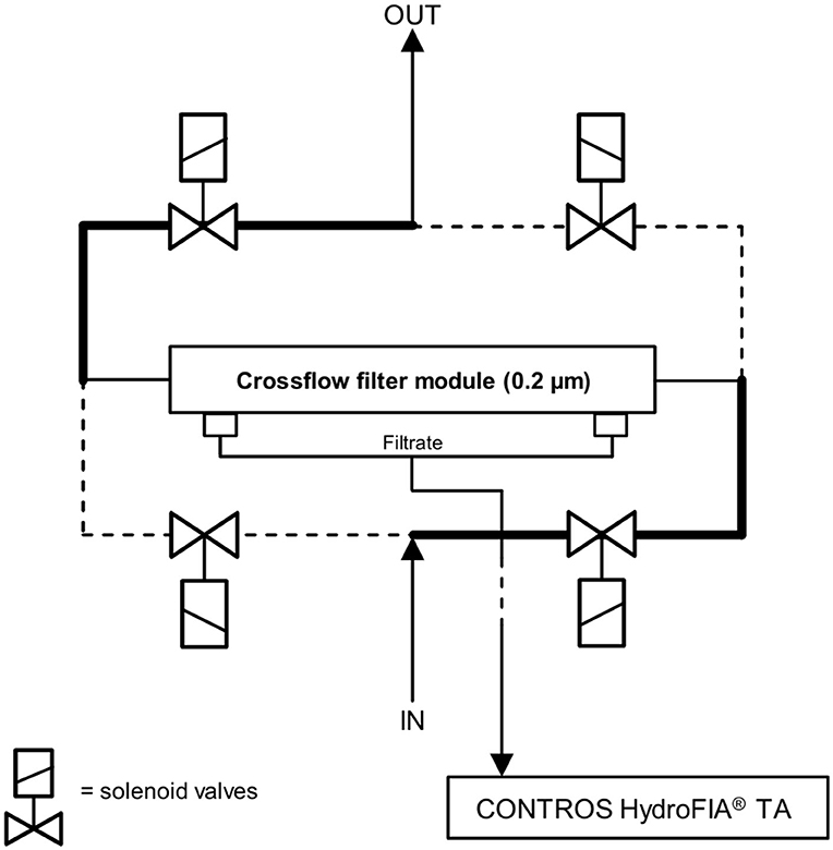
Figure 1. Schematic illustration (not to scale) of the crossflow filter device. The black bold solid lines and the black dashed lines represent the two respective flow paths achieved by opening and closing the solenoid valves.

2.1.3. Temperature and Salinity Measurements

For measuring the intake seawater temperature, a SBE 38 Digital Oceanographic Thermometer (Sea-Bird Electronics, USA) is used as an inline temperature sensor. The salinity of the seawater is determined by a SBE 21 SeaCAT Thermosalinograph (Sea-Bird Electronics, USA). Both sensors are calibrated annually by the manufacturer.

2.2. Large-Volume Reference Seawater Storage Test

2.2.1. Containers

For the purpose of stable storage of a larger volume of reference seawater, we tested several container types. The following criteria were important for our selection: (1) Handling on moving platforms like ships, (2) inertness of the inner material, (3) headspace above the seawater, (4) gas permeability, and (5) cost. Table 1 gives an overview of all tested containers. The numbering in Table 1 is for classifying the containers, where 1.x are gas sampling bags, 2.x are infusion bags, and 3.x are inflexible containers.

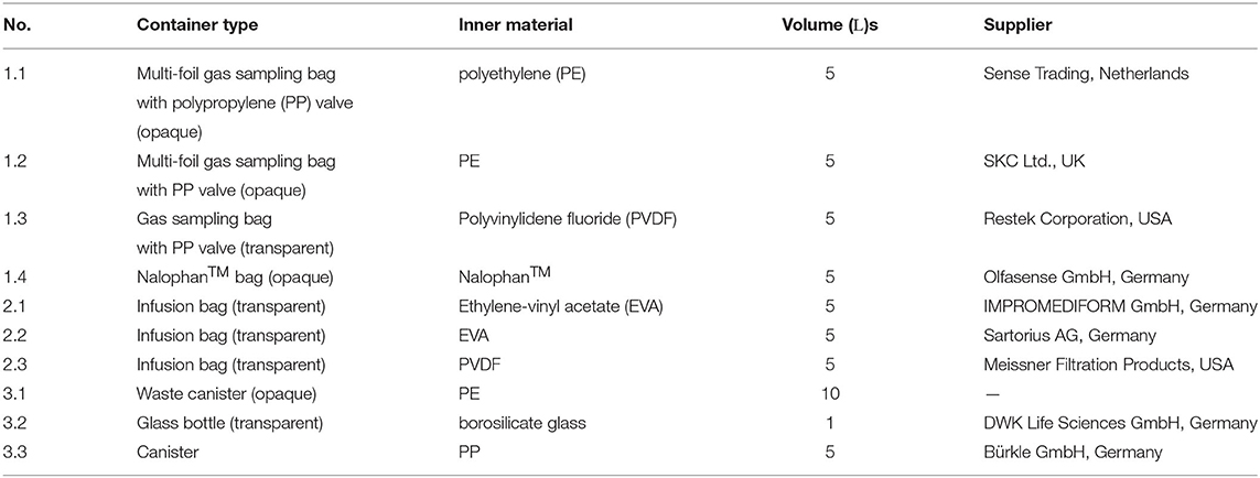
Table 1. Tested containers for large-volume reference seawater storage.

2.2.2. Stability Tests

To test each container for seawater TA stability over time, it was filled with about 5 L of a poisoned seawater sample and stored at a dark place to prevent biological growth. This seawater sample was prepared by diluting concentrated seawater solutions (“Absolute Ocean,” ATI Aquaristik, Germany) and adding mercury chloride for stabilization (similar to CRM conditions). Its absolute TA value had to be within the working range of the analyzer as only the temporal change between the starting value and the value after x days was of interest. The resulting TA value was similar to that of the CRM (≈ 2,215 μmol kg^-1), as measured by the CONTROS HydroFIA^Ⓡ TA in the laboratory. Each measurement day started with stabilization measurements and a “calibration” of the system with a freshly opened CRM. This procedure assured accurate and comparable measurements.

For determining the initial TA value (TA_start) of the seawater at the start of the storage experiment, the freshly filled container was connected to the analyzer and five repetitive measurements were carried out. TA_start therefore is the mean of these five measurements. After x days, the measuring procedure was repeated with a maximum storage time of 30 days (x_max = 30). The TA value after x days (TA_x) was calculated by averaging the five measurements on day x. For evaluating the TA stability over time, the difference (ΔTA_x) between TA_start and TA_x was calculated for each day and container.

2.3. North Atlantic SOOP Line

2.3.1. The Ship

Since 2018, the merchant vessel M/V Atlantic Sail operated by Atlantic Container Line (ACL) serves as SOOP line in the subpolar North Atlantic Ocean under the responsibility of our working group at the GEOMAR Helmholtz Centre for Ocean Research Kiel. It is a hybrid roll-on/roll-off container vessel (ConRo). This line is an official ocean observation station (DE-SOOP-Atlantic Sail) of the European research infrastructure “Integrated Carbon Observation System” (ICOS). The ship operates between Europe (Hamburg, Germany; Antwerp, Belgium; Liverpool, UK) and North America (Halifax, Canada; New York, USA; Baltimore, USA; Norfolk, USA). A full roundtrip of the ship takes about 5 weeks. Any maintenance of our installations is typically carried out during port calls in Hamburg, Germany. The seawater measurements are only carried out during the trans-Atlantic crossings between Liverpool, UK and Halifax, Canada.

2.3.2. Onboard Installation

All facilities and instruments related to surface seawater measurements are installed on the lowest level of the engine room at the port side of the ship. Figure 2 shows a schematic illustration of the installations, where valve #1 is a pneumatic valve, and valves #2–4 are manual ball valves. Details about individual components can be found in section 2.1. Photos of the onboard installation can be found in the (Supplementary Figure 1).

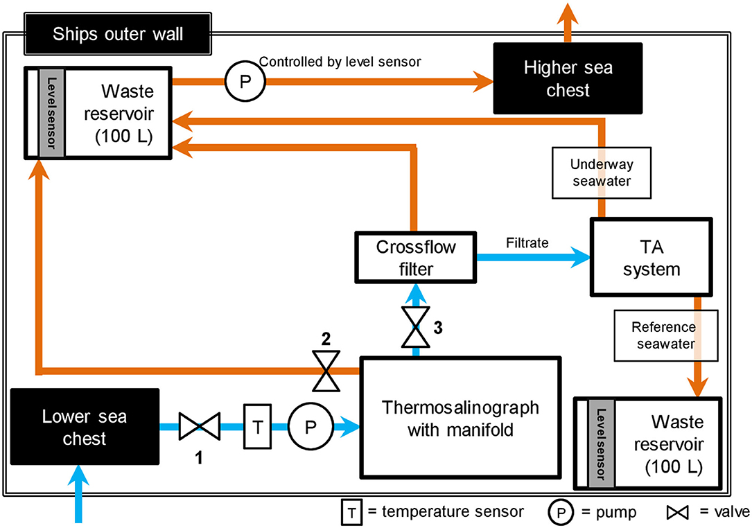
Figure 2. Schematic illustration (not to scale) of the onboard installation for seawater measurements. Black filled boxes represent ship facilities. White filled boxes represent our installations. Blue arrows, and orange arrows represent the water flow of fresh seawater, and waste seawater, respectively.

The ship's lower sea chest was chosen as seawater intake. Its intake is located about 8-11 m below sea surface depending on the draught of the ship, which varies with cargo load. A centrifugal pump delivers seawater to the system. The seawater intake temperature is continuously measured with an inline temperature sensor (SBE 38). In order to split the seawater flow, a manifold with an integrated thermosalinograph (SBE 21) is installed. It provides the pCO₂ system and the crossflow filter device for TA measurements with fresh seawater at a flow rate of 3 and 1 L min^-1, respectively. The TA system only measures the filtrate of the crossflow filter. All waste seawater (with exception of measured TA reference seawater) flows into a 100 L reservoir with a level sensor that controls a second centrifugal pump, which empties the content into the ship's higher sea chest when full. From there, the waste water leaves the ship into the ocean. The measured reference seawater from the TA system is collected in a separate 100 L waste container as it is poisoned with mercury chloride. When this waste reservoir is full, its level sensor turnes off the CONTROS HydroFIA^Ⓡ TA, which serves as an emergency stop and prevents an overflow of the poisoned waste reservoir.

The main electric management of the entire system is organized in an electric box (Supplementary Figure 1). This box also contains a computer, which controls all serially controllable devices such as the CONTROS HydroFIA^Ⓡ TA. Furthermore, the main switch is located there, which allows for easy the starting and stopping of the complete system by member of the crew.

2.3.3. Autonomous TA Measurement Procedure

Figure 3 shows the schematic set-up of the TA analyzer installation. The current version of the analyzer is equipped with two inlets: One for continuous (inlet 1) and one for discrete measurements (inlet 2). In our SOOP application, inlet 2 is permanently connected to the reference seawater storage. Inlet 1 is connected to a 3/2-way pinch valve (#1) obtained from Bio-Chem Fluidics, USA, which can be electrically actuated. When not actuated, the analyzer receives seawater from the crossflow filter. When actuated, inlet 1 is connected to a 5 L reservoir of deionized (DI) water. A second 3/2-way pinch valve (#2) downstream the system's outlet controls the waste water separation. When not actuated, the waste is routed to the regular seawater waste reservoir. When actuated, the waste water is routed to the poisoned waste reservoir. Both pinch valves are wired with the programmable outlet strip “MultiBox-pro seri” obtained from ANTRAX Datentechnik GmbH, Germany. Each socket of this outlet strip can be switched on or off via serial commands. The TA analyzer is also controllable via serial commands. Therefore, both the CONTROS HydroFIA^Ⓡ TA as well as the MultiBox are connected to the computer.

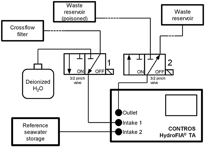
Figure 3. Schematic illustration (not to scale) of the onboard installation for seawater TA measurements.

The workflow of the autonomous TA measurements in unattended SOOP line mode is illustrated in Figure 4. During all named phases, the status of the main switch is permanently controlled by a software program written in Python. This script additionally sends and reads all serial commands to and from the analyzer and the MultiBox. By triggering the main power switch of the system and thereby starting the seawater flow, the stabilization phase of the analyzer is initiated. Both pinch valves are not actuated. The analyzer carries out 30 consecutive measurements using inlet 1 every 10 min. After these measurements, the analyzer starts with the actual measurement cycle. It consists of two parts: (1) Five consecutive reference measurements at 10 min interval using inlet 2 with actuated pinch valve #2 and not actuated pinch valve #1, and (2) 96 consecutive surface seawater measurements (underway) at 15 min interval using inlet 1 with both pinch valves being not actuated. This measurement cycle always starts with reference measurements and is only interrupted by switching off the main switch, which initiates the final flushing phase. During this phase, pinch valve #1 is actuated for 300 s and #2 is not actuated. Meanwhile, the system flushes its inner tubing with DI-water and stops all measurements until the main switch is actuated again. In case the main switch is turned off during the stabilization phase, the analyzer skips the measurement cycle and directly starts with the flushing phase.

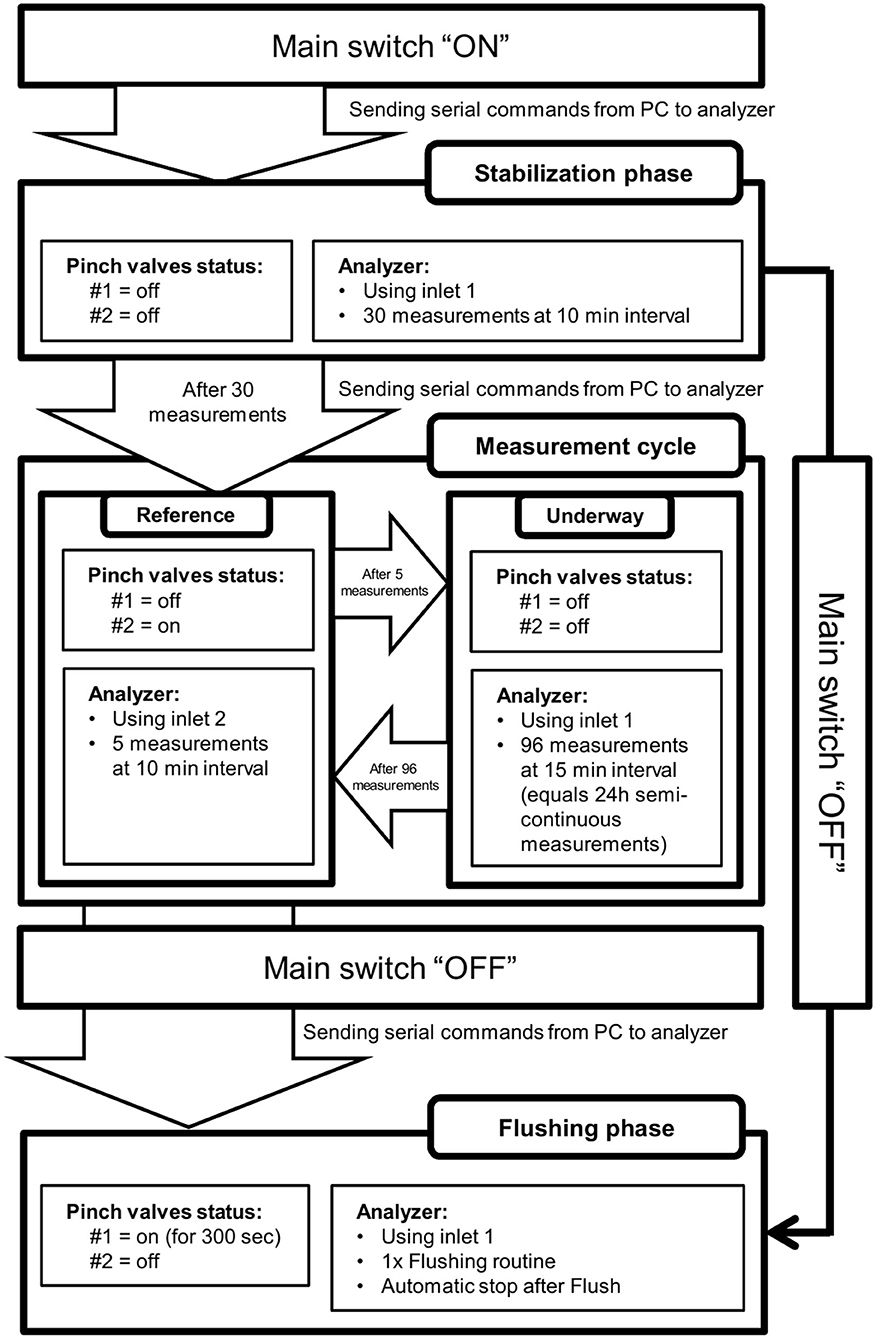
Figure 4. Workflow of the autonomous TA measurements.

2.3.4. Cleaning Procedure

Previously gained experiences with the analyzer show that a flush with DI-water at the end of a measuring campaign and before longer idling times (more than 48 h) prevents the formation of deposits in the inner tubing and therefore enhances the long-term stability of the analyzer. It is also recommended by the manufacturer. The automated final flushing phase (see Figure 4) is the easiest way to assure the best conditions for the idling state between two measuring campaigns, i.e., the DI-water remains in the tubing and the system stops until the seawater flow is restarted.

2.3.5. Stabilization Measurements

Due to the DI-water in the tubing during idling times, the analyzer shows only a brief initial drift, when the measurements are restarted. Consequently, only a moderate number of stabilization measurements are necessary before the first reference seawater analyses. The number of such measurements mostly depends on how long the previous idling time was. Our first study with the analyzer revealed that the shorter the idling times are, the fewer stabilization measurements have to be carried out (Seelmann et al., 2019). However, this behavior requires that the analyzer continuously measures during the measuring phase. Furthermore, idling times of less than 48 h show no initial drift and a stabilization phase is not needed. As the idling times on our SOOP line are at least 7 days, we decided to carry out 30 consecutive underway measurements with a measuring interval of 10 min during the stabilization phase. This high number of measurements includes a safe buffer for even longer idling times to guarantee stable conditions for subsequent analyses. After the stabilization, the measurement routine starts with the reference seawater followed by the measurement cycle (see Figure 4).

2.3.6. Waste Handling

Due to the poisoning of the reference seawater with mercury chloride, the waste water has to be collected separately after measurement and properly disposed. The waste from regular underway measurements is unproblematic for the environment and therefore it is disposed with the waste water of the pCO₂ installation (see Figure 2). As the analyzer has only one outlet, we initially collected the entire waste water in the poisoned waste reservoir, whether it was from reference or underway measurements, and emptied the 100 L canister during port calls in Hamburg, Germany to dispose it properly. But this procedure was too laborious and time consuming. During 1 month of operation, about 50 L waste water are collected, which results in high emptying frequencies and disposal costs. Consequently, we installed an electrically actuated 3/2-way pinch valve downstream the analyzer's outlet. As long as the system measures underway seawater, the valve is not actuated and the waste water is routed into the regular waste reservoir, which is emptied into the ocean. During reference measurements, the valve is actuated and the waste water is routed to the poisoned waste reservoir. This procedure reduces the volume of the collected hazardous waste water to 2.5 L per month (with daily reference measurements of five consecutive single measurements). Through this waste separation routine, we are able to strongly reduce our maintenance effort during port calls and the disposal costs.

2.3.7. Discrete Samples

In order to supervise and evaluate the new installation, we participated in the first two cross-Atlantic transits onboard the vessel: (1) From Liverpool, UK to Halifax, Canada (30 October 2018–06 November 2018), and (2) from Halifax, Canada to Liverpool, UK (05 February 2019–11 February 2019). During these transits, discrete samples for TA and DIC were collected three times per day as soon as the ship reaches the open ocean. They were bottled, poisoned and air-tight sealed following the recommendations of Dickson et al. (2007). Their measurement took place in the home laboratory (GEOMAR Helmholtz Centre for Ocean Research Kiel, Germany) using a standard open-cell alkalinity system with potentiometric titration (VINDTA 3S, Marianda, Germany) with an accuracy of about ± 2 μmol kg^-1 (daily quality assurance using CRM). These measurements also followed the recommendations of Dickson et al. (2007). The TA values of the discrete samples (TA_ref) were used for accuracy evaluation and proof of the successful implementation of the CONTROS HydroFIA^Ⓡ TA analyzer. Besides the discrete sampling, no further interference with the unattended character of the installation onboard the ship occurred.

3. Results and Discussion

3.1. Large-Volume Reference Seawater Storage Tests

The main issue during autonomous long-term installations of the analyzer is the provision of enough reference seawater for regular quality assurance and drift correction. As 500 mL standard CRM bottles are insufficient for longer measurement campaigns, we tested several different container types in the laboratory.

Before we started with the actual testing, we set certain stability requirements, which needed to be fulfilled by the container: After 30 days of storage, each ΔTA_x (including analyzer uncertainty) need to fall within the ± 10 μmol kg^-1 uncertainty range required by ICOS for ship-based TA measurements. This requirement is based on the “weather goal” introduced by Newton et al. (2015). International intercomparison measurements on discrete measurement with shore-based instrumentation showed that most of the participating laboratories reached that goal, but only few achieved the “climate goal” (± 2 μmol kg^-1) (Bockmon and Dickson, 2015). Ideally, the ΔTA_x values would fall within the ± 2.2 μmol kg^-1 uncertainty range of the analyzer. This value is based on the systems typical relative uncertainty of 0.1 % at a reference seawater TA of ≈ 2,215 μmol kg^-1 demonstrated under field conditions (Seelmann et al., 2019).

Figure 5 shows the results of the container stability tests without the standard error of the five repeated measurements at each point as the small numbers would not be properly visible with the y-axis scaling. Clearly, most of the tested containers do not meet the requirements. Gas sampling bags and infusion bags made out of materials such as PE or EVA (numbers: 1.1, 1.2, 2.1) show a clear trend toward decreasing TA in the stored seawater. The same behavior is observed with the canisters made of PE and PP (numbers: 3.1, 3.3). We hypothesize that these materials contaminate the seawater with chemical substances, which bind or consume TA relevant compounds. The infusion bag #2.2, which is also made of EVA, only shows a slight decrease in TA at the beginning followed by a subsequent increase after 24 days. This behavior suggests that the material causes less contamination with the increase in TA being most likely caused by evaporation of water by the permeation through the foil. The majority of the ΔTA_x of #2.2 lies within the ICOS uncertainty range, but only very close. The gas sampling bag #1.4 made of Nalophan™ shows a mostly increasing ΔTA_x behavior. We hypothesizes that its barrier layer is not able to prevent water evaporation and/or initially releases alkalinity into the water. The infusion bag #2.3 made of PVDF shows a more unspecific, but highly unstable behavior and is therefore not suitable.

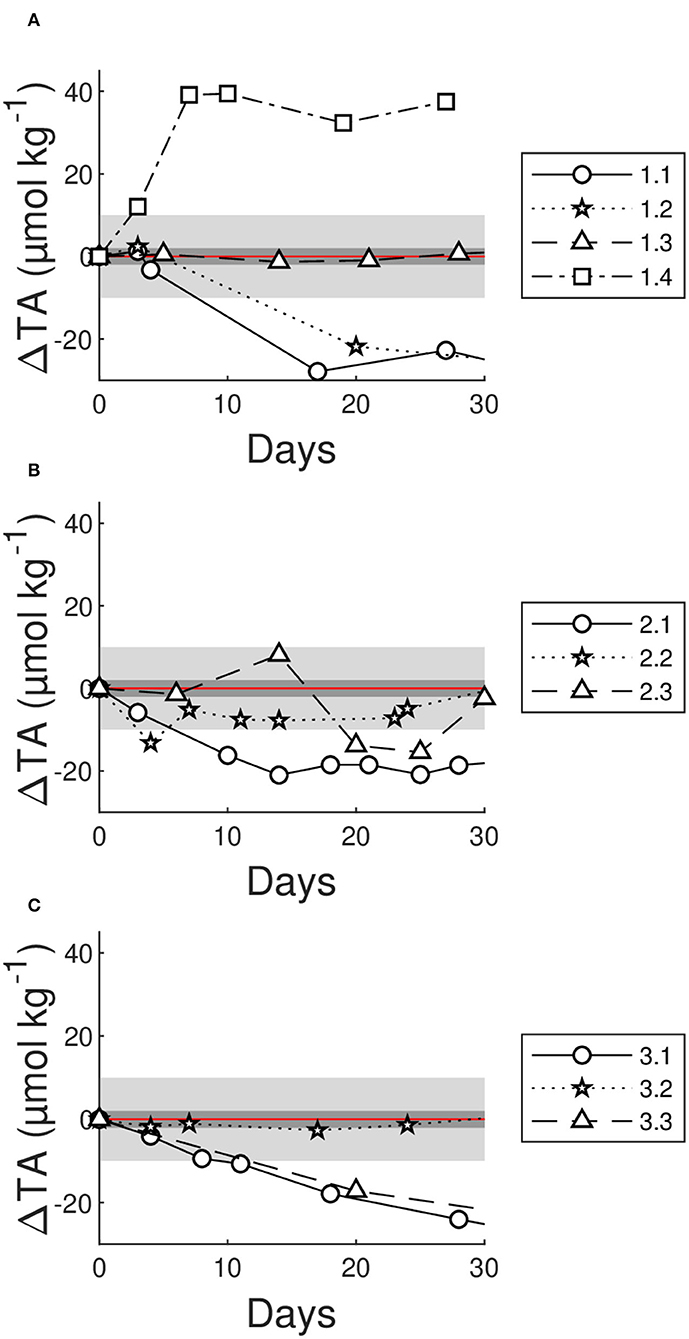
Figure 5. Difference between measured TA after x days and TA_start (ΔTA_x) for each container type as a function of the measurement day x, where (A) shows the gas sampling bags, (B) the infusion bags, and (C) other container types. The numbers in the legend represent each tested container following the numbering in Table 1. The horizontal red line in each plot represents ΔTA_x = 0 μmol kg^-1. The light gray and the dark gray areas indicate the ICOS required uncertainty of ± 10 μmol kg^-1, and the analyzers typical relative field uncertainty of 0.10 % (equals ± 2.2 μmol kg^-1 at TA = 2215 μmol kg^-1) (Seelmann et al., 2019), respectively.

The most promising solution for a large-volume seawater storage is container #1.3. It fulfills both stability requirements with an average difference of (0.2 ± 1.3) μmol kg^-1 over 30 storage days. But also the glass bottle (#3.2) stores the seawater in a comparably stable way. However, inflexible containers like bottles always have the problem of a constantly increasing headspace above the seawater and therefore, enhanced evaporation of water. This results in increasing TA values over time. Although such a behavior does not show up in Figure 5C, it has to be taken into account that the tested bottle only had a volume of 1 L. For unattended long-term measurements of the analyzer on SOOP lines, larger volumes of 5 L or more are preferable. Most likely the influence of the headspace is much stronger in a 5 L bottle. That the headspace does not affect the TA in the other large inflexible containers (#3.1 and #3.3) may be because of the counteractive material effects. Therefore, we hypothesize that material effects from PE or PP are much stronger than headspace effects. Another disadvantage of the glass bottle is that its handling on a moving ship is not as straightforward as that of a flexible bags. Consequently, we decided to choose the PVDF gas sampling bag (#1.3) as large-volume storage for the reference seawater.

3.2. First Unattended Measurement Campaigns

3.2.1. Cruise Tracks and TA Time-Series

Figure 6A shows the cruise tracks of the first four campaigns on the North Atlantic SOOP line, where the CONTROS HydroFIA^Ⓡ TA analyzer was installed and measured.

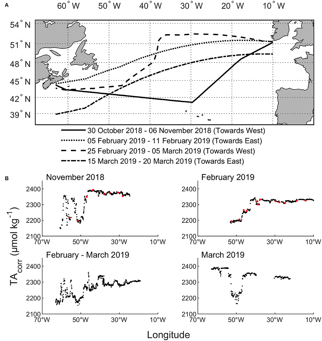
Figure 6. (A) Cruise tracks of the first four campaigns on the North Atlantic SOOP line. (B) TA values corrected for instrument drift during the first four measuring campaigns as a function of the measured longitudes. Each filled red circle represents the TA value of a discrete sample taken at a certain time. Both plots on the left are from westward crossings, and both plots on the right are from eastward crossings.

To give an overview of the measured TA values in the monitored region during the first four measuring campaigns, Figure 6B shows the TA vs. the measured longitudes. The red filled circles in both plots on the top represent the TA value of the discrete samples. Due to problems with the thermosalinograph, the measurement start of the analyzer was delayed during the November 2018 transit. The delayed start in February 2019 was due to a problem with the ship's sea chest. Throughout all campaigns, a total of 1700 TA measurements were performed by the analyzer at a measurement interval of 15 min.

The shown underway TA values are fully post-processed, which means that the typical drift of the analyzer was corrected for by using the daily reference measurements from the storage bag. The complete correction procedure is not provided here, but can be found in Seelmann et al. (2019). Furthermore, a detailed scientific interpretation of the shown underway data is not part of the report. Here, the main focus lies on the performance assessment of the analyzer in unattended SOOP mode.

3.2.2. Data Quality

In order to evaluate the accuracy of the TA values acquired in continuous operation mode with the PVDF gas sampling bag as large-volume reference seawater storage, discrete samples were taken throughout the first two trans-Atlantic crossings (November 2018 and February 2019). Figure 7 shows the comparison between the drift-corrected TA values measured with the CONTROS HydroFIA^Ⓡ TA analyzer and the TA of discrete samples measured with the reference open-cell titrator VINDTA 3S. The averaged residuals between the two measurement systems were (−0.2 ± 4.7) μmol kg^-1 for the November 2018 campaign, and (−0.5 ± 4.3) μmol kg^-1 for the February 2019 campaign. Furthermore, a slightly increasing drift is still visible in both plots, which might be caused by the PVDF gas sampling bag. Although the bag showed stable TA values under laboratory conditions (see Figure 5), the changing conditions in the ship's engine room appear to deteriorate its ability to stably store the seawater. However, on average the analyzer shows no systematic offset, but the variation around the mean value is less accurate than the typical field accuracy observed during our previous characterization study (-0.3 ± 2.8 μmol kg^-1). It must be considered that the latter accuracy determination was based on daily CRM measurements (overall 15 measurements of five consecutive single measurements) using freshly opened CRM bottles each day (Seelmann et al., 2019), and it therefore represents a best case scenario. Furthermore we would like to note that the matching of autonomous underway measurements with data from discrete sampling is a complicated matter especially under conditions of high TA variability such as in the western part of the region. Imperfect matching between discrete samples and underway measurements (e.g., mismatching in sampling time) inevitably introduces an additional element of noise which cannot be avoided even with greatest care in the matching. The accuracy and its variation is strongly effected by the stability of the CRM, and logically, we expected a slight accuracy deterioration when the CRM is stored in the large-volume PVDF gas sampling bag as compared to the original bottle. The high accuracy requirement (≤ ± 2 μmol kg^-1) for standard TA open-cell titrators described by Dickson et al. (2007) can only be fulfilled by the mean offsets of −0.2 and −0.5 μmol kg^-1. However, the overall uncertainty of the systematic error is deteriorated due to the larger variation of the observed residuals. As long as there is no other stable option for the reference storage during long-term deployments, it must be accepted that the uncertainty of the possible bias is extended compared to freshly opened CRM bottles.

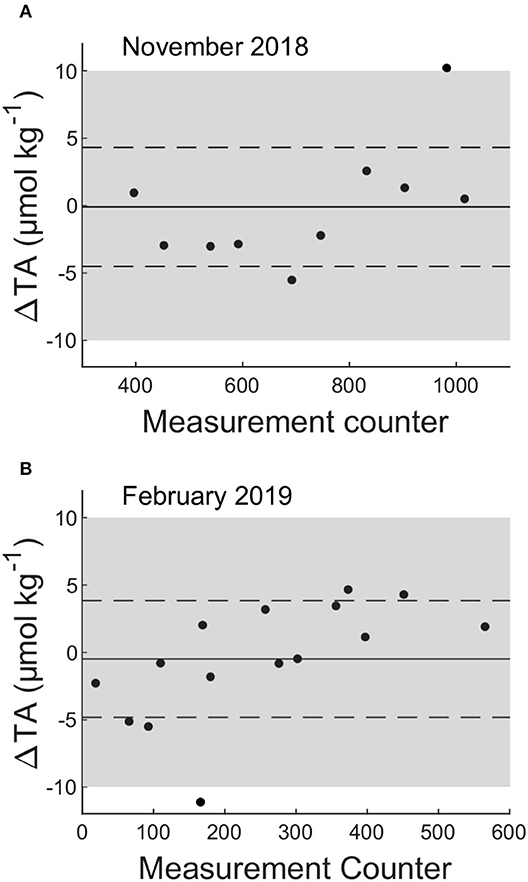
Figure 7. Residuals of the intercomparison of TA measurements between the CONTROS HydroFIA^Ⓡ TA (drift corrected values) and the reference open-cell titrator (VINDTA 3S) for (A) the November 2018, and (B) the February 2019 transit. The horizontal black solid line indicates the averaged bias, $\overline{\Delta \text{TA}}$, and the horizontal black dashed lines indicate $\overline{\Delta \text{TA}}\pm \sigma$ (−0.2 ± 4.7 μmol kg^-1 for November 2018, and −0.5 ± 4.3 μmol kg^-1 for February 2019). The gray area represents the uncertainty of ± 10 μmol kg^-1 required by ICOS.

Throughout all measurement campaigns, the short-term precision of the analyzer (standard deviation of the consecutive reference measurements) exhibits the typical field precision of ± 1.1 μmol kg^-1 found during our previous characterization study. Therefore, the usage of the PVDF gas sampling bag as large-volume reference seawater storage does not affect the random error of the measurements. For this reason we do not show any further precision evaluation here.

We can conclude that the quality of the TA data achievable with our SOOP line installation is mostly affected by the reference seawater storage. The usage of a the PVDF gas sampling bag appears to introduce a small additional uncertainty by a slightly increasing drift while not affecting the short-term precision. Furthermore, on average, no systematic offset is introduced by the reference material storage. The entire data quality (accuracy and precision) provided by the installed analyzer fulfills the uncertainty criteria of ± 10 μmol kg^-1 for ship-based TA measurements on ICOS stations.

3.2.3. Comparison With TA Parameterization and Its Limits

In order to evaluate the consistency between the TA data measured with the installed analyzer and the typical TA range and variability in the monitored region, we compare the measured TA values to TA predicted from sea surface salinity (SSS) and sea surface temperature (SST) values using the parameterization of Lee et al. (2006). For the North Atlantic, the prediction follows the equation

which is valid between the latitudes 30°N and 80°N, for the SST range 0°C to 20°C, and for the SSS range 31–37. Hence, only TA values measured within these ranges are compared with the respective predicted values.

The consistency is estimated by calculating the root mean square error (RMSE) following

where n is the number of TA measurements.

Figure 8 shows the results of the comparison by plotting the drift-corrected TA values measured with the analyzer (TA_corr) vs. the predicted TA values (TA_pred). The resulting linear correlations include the uncertainties of TA_corr and TA_pred using the MATLAB™ script provided by Thirumalai et al. (2011) based on the statistical method described by York et al. (2004).

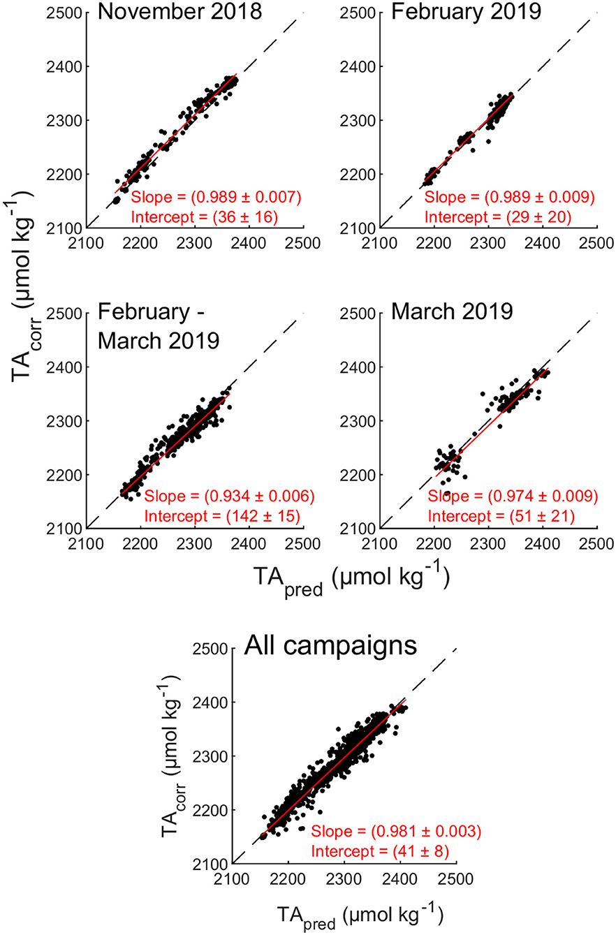
Figure 8. TA values (after drift correction) measured by the analyzer (TA_corr) as a function of the predicted TA values (TA_pred) using the established parameterization described by Lee et al. (2006) for each measuring campaign, and for all campaigns together. The black dashed lines indicate the 1-to-1 line of the plot. The red solid lines represent the linear correlation between TA_corr and TA_pred with their slopes and intercepts given in each plot.

Throughout all measuring campaigns, the correlation between TA_corr and TA_pred is not fully satisfactory with a slope of (0.981 ± 0.003) and an intercept of (41 ± 8). A perfect correlation would result in a slope of 1 and an intercept of 0 within their uncertainties. The four single trans-Atlantic crossings show similar results (see Figure 8). The average RMSE for all campaigns is calculated at ± 12.3 μmol kg^-1 following equation 2, and is therefore barely satisfactory, too. A satisfactory RMSE would be a maximum of ± 11.4 μmol kg^-1, which is a combination of the uncertainty of the parameterization (Lee et al., 2006) and the underway measurements. However, the intercomparison with discrete samples confirms the sufficient accuracy of the data obtained with the autonomous TA analyzer, which means that these biases must be due to other reasons.

In order to discover these reasons, we compare our data set with the Global Data Analysis Project v1.1 (GLODAPv1) (Key et al., 2004) from 1990 to 1998, which was used by Lee et al. (2006) for deriving their parameterization. Figure 9 shows this comparison, which reveals the fundamental limits of the used parameterization and, hence, possible reasons for the observed biases:

1. Spatial bias: The comparison of the spatial distribution of both data sets in the North Atlantic (see Figure 9A) reveals that the GLODAPv1 data set has an underrepresented area (38°N – 50°N, 35°W – 65°W) into which about 60 % of our measured TA values fall. Two major currents meet in this region: The warm and salty North Atlantic Current from the Southwest, and the cold and fresh Labrador Current from the North. Hence, this significant mixing area is not adequately represented in the parameterization by Lee et al. (2006), which may lead to biases. In order to prove that there is a spatial bias induced by this underrepresented area, the RMSE is re-calculated only for this area (RMSE_West), and without this area (RMSE_East), respectively, resulting in RMSE_West = 14.2 μmol kg^-1 and RMSE_East = 9.7 μmol kg^-1. These results obviously prove the existence of the spatial bias. Another direct consequence of the underrepresented area is that values of 2,100< TA <2,300 μmol kg^-1, and 31 <SSS<34.5 are also underrepresented in the parameterization due to the missing influence of the cold and fresh Labrador Current (see Figure 9B), although Lee et al. (2006) confirmed a SSS validity from 31 to 37.

2. Temporal bias: Due to the fact that the parameterization is based on data from between 1990 and 1998, any changes in SSS and SST caused by changes in the hydrological cycle, global warming over the last decades, etc. are not considered. SSS and SST changes may influence the relationships between SSS, SST and TA, and therefore, the corresponding parameterization coefficients. A comparison of the TA-SSS-relation based on the GLODAPv1 data and the SOOP-based data (see Supplementary Figures 2A,B) revealed small changes in the slope and intercept. These changes may point at TA and SSS changes over the last 20 years. However, it must be taken into account that they could be also caused by seasonal biases (see point no. 3). Furthermore, a comparison of the SST-SSS-relationships of both data sets (see Supplementary Figure 2C) reveals a shift in SST to slightly higher values at salinities <34 over the last 20 years, although the SOOP-based data were only measured during fall/winter times, and the GLODAPv1 data set is mostly based on spring/summer data. This may be a direct consequence of the global warming over the last decades. However, a far better direct comparison of the TA, SSS and SST data is possible as soon as we have measurements dated from spring/summer times.

3. Seasonal bias: Figure 9B shows the comparison of the months, when the TA values were measured. Clear most of the TA data used by Lee et al. (2006) were acquired during spring and summer times, whereas our data were measured during fall and winter times. Throughout the year, different biogeochemical processes take place in the surface ocean affecting the TA, i.a. CaCO₃ formation during summer. As most of the parameterization data were acquired during summer, the influence of such processes may not apply to winter times, and vise versa, which may lead to biases.

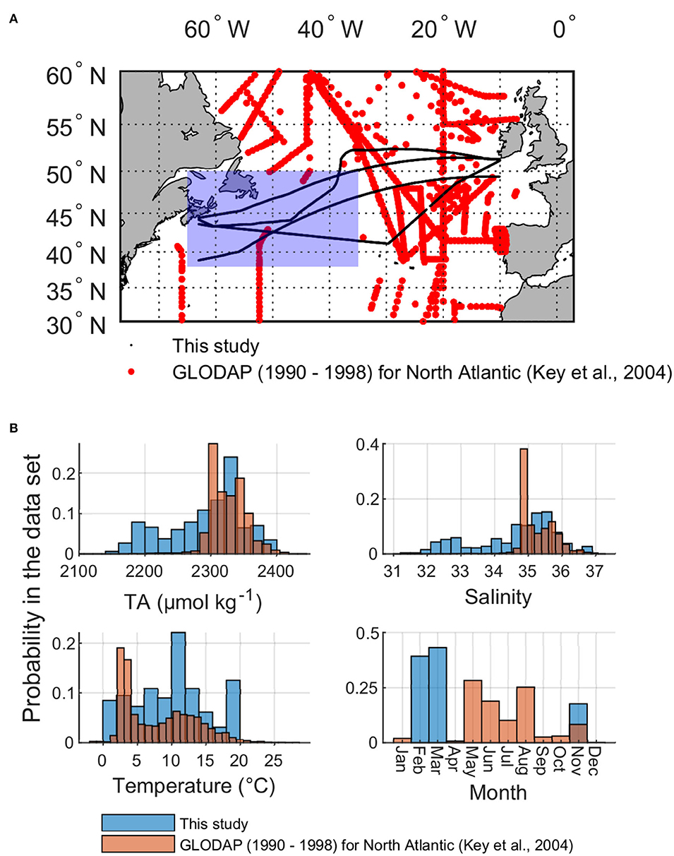
Figure 9. (A) Spatial distribution of our measured data (black) and the GLODAP data set between 1990 and 1998 (red) for the North Atlantic (30°N - 60°N). The blue patch represents the area, which is underrepresented in the parameterization by Lee et al. (2006). (B) Histograms of observations of TA, salinity, temperature, and month of observation in the data set of this study (blue) and the GLODAP data set (orange).

Supplementary Figure 3 shows the residuals between the measured TA values (TA_corr) and the predicted TA values (TA_pred) over the cruise tracks of the trans-Atlantic crossings, and as a function of SSS and SST. There, the spatial and seasonal biases are pointed out in particular. However, a detailed discussion of these residuals is not part of this report, as it only forms the explanation basis for the biased TA comparison.

Supplementary Figure 4 shows the additional comparison of the SOOP-based TA data and their TA-SS-relationship with the TA-SSS-relationship described by Millero et al. (1998) for the Atlantic Ocean. Also this comparison results in a not fully perfect agreement. However, it has to be taken into account that the TA-SSS-relation of Millero et al. (1998) counts for the whole Atlantic Ocean and not only for the North Atlantic Ocean as the parameterization described by Lee et al. (2006). Furthermore, this comparison is meant to be more informative, and, therefore, a detailed discussion is not part of this report.

The not fully perfect agreement between our SOOP-based TA observations and TA predictions points at regional and seasonal limitations in the GLODAPv1 database which can lead to biases in TA predicted by parameterizations based on GLODAPv1 such as that by Lee et al. (2006). This points at the need better spatiotemporal coverage of surface ocean TA observations, which are now possible with the method described here. Future work will aim at a new regional SSS and SST based TA prediction scheme based on the data sets provided by our North Atlantic SOOP line (see section 5).

4. Summary

In this study, we present a ship-board installation scheme for autonomous underway TA measurements using the novel CONTROS HydroFIA^Ⓡ TA analyzer on a Ship of Opportunity operating in the North Atlantic Ocean. The here described setup addresses the major issues arising from autonomous TA measurements using this analyzer: (1) Regular reference measurements including the provision of sufficient CRM volume, (2) an automated DI-water flushing routine before idle times, (3) stabilization measurements at the beginning of a measuring campaign, and (4) separation of the waste water depending on underway or reference measurements.

Stability tests with different large-volume container types used as reference seawater storage revealed that the inner material of the container can strongly influence the long-term TA stability. Synthetic materials like PE, PP or EVA were found not suitable as they reduce the TA value by most likely contaminating the seawater with unknown chemical compounds. Borosilicate glass bottles, which are used as CRM bottles with a volume of 500 mL, seem to be a stable alternative, but due to their inflexible character, there could be problems with the increasing headspace in the bottle, especially with larger volumes over 5 L or more. The only promising container was a 5 L gas sampling bag made of PVDF. During a test period of 30 days, the seawater TA on average only varied by (0.2 ± 1.3) μmol kg^-1. The bag therefore was deemed suitable as long-term reference seawater storage. Throughout all presented measurement campaigns on the SOOP, this bag was used for reference measurements.

The automated cleaning and waste separation procedures can be easily implemented by using electrically actuated 3/2-way pinch valves and a control software sending and receiving respective serial commands. The stabilization phase after idle times is set to 30 consecutive underway measurements and also implemented in the software. We conclude that all previously observed issues can be solved by our installation.

The success of the autonomous TA measurement implementation on our SOOP line was verified by intercomparison with measurements performed by a reference open-cell titrator. During the first two campaigns, the overall agreement between the autonomous TA measurements and the reference system was (-0.2 ± 4.7) μmol kg^-1 (November 2018) and (−0.5 ± 4.3) μmol kg^-1 (February 2019). Although the variation around the bias slightly deteriorates in comparison to the typical accuracy of (−0.3 ± 2.8) μmol kg^-1 observed when using freshly opened CRM bottles, the analyzer still met the uncertainty requirement of ± 10 μmol kg^-1 for ship-based ICOS stations. The deterioration of the systematic error variation was most likely due to the usage of the large-volume CRM storage instead of freshly opened CRM bottles. However, the random error of the analyzer was not affected by this and still featured the typical precision of ± 1.1 μmol kg^-1.

A comparison with predicted TA values based on a established parameterization revealed biases between measured and predicted TA values. These biases are mostly due to imperfect spatiotemporal coverage in the GLODAPv1 data set used in establishing the parameterization. This points at the need surface ocean TA observations with better spatiotemporal coverage like it is now provided by our installation on the North Atlantic SOOP line.

Summing up, we can say that the implementation of the novel autonomous TA analyzer CONTROS HydroFIA^Ⓡ TA on a commercial SOOP line was fully successful. The achieved TA values are in full agreement with the ICOS quality requirements and therefore, in combination with pCO₂, perfectly usable for the characterization and long-term observation of the marine inorganic carbon system. This novel technology makes much improved spatiotemporal coverage of surface ocean TA from the carbon-SOOP network now possible.

5. Future Data Applications

The addition of TA as second operationally measured variable to SOOP will add tremendously to the interpretation potential of SOOP-based data. Due to the access to the complete speciation and all variables of the inorganic carbon system, future work will aim at investigations on various drivers and causes of observed inorganic carbon perturbations in the subpolar North Atlantic, e.g., ocean acidification, decadal and seasonal TA trends (similar to the work described by Macovei et al., 2020), or changes in productivity and calcification.

Although the interpretation potential of SOOP-based data increases by measuring TA as second carbonate variable, it is limited to surface measurements, i.e., investigations on changes in the vertical dimension of the marine inorganic carbon system are not possible. The Biogeochemical-Argo (BGC-Argo) program wants to overcome this observational gap by equipping their BGC-Argo floats with pH sensors (Claustre et al., 2020). However, the installed pH sensors show a significant drift over time, and therefore must be calibrated on regular basis. A future collaboration of our SOOP line with the BGC-Argo program will aim at a calibration procedure, which uses surface pH values calculated from the SOOP-based pCO₂ and TA measurements.

Another important future data application is the work on an improved TA parameterization. As soon as we have collected enough data from our SOOP line (minimum 1 year of semi-continuous measurements), we want to establish a TA parameterization similar to the one described by Lee et al. (2006). Their SSS and SST fitting was based on 326 data points in the North Atlantic collected between 1990 and 1998 during spring and summer times. Our future parameterization would be based on about 12,000 TA data points from 1 full year with very good spatial coverage of the North Atlantic, and could be expanded by more data afterwards. Furthermore, there will be the possibility to include seasonal variability into the calculation scheme as we measure TA throughout the year.

Data Availability Statement

The raw data supporting the conclusions of this article will be made available by the authors, without undue reservation.

Author Contributions

KS performed the laboratory and field work. TS and KS performed the installation onboard the ship. KS, SA, and AK performed the data analysis. KS performed the statistical analysis, and data visualization. KS wrote the first draft of the manuscript. All authors contributed to the conception and design of the study, manuscript revision, read, and approved the submitted version.

Funding

This research was supported by the European Horizon 2020 projects AtlantOS (#633211) and RINGO (#730944), the project ICOS-D (#01LK1224J) of German Federal Ministry of Education and Research, the project Digital Earth of the Initiative and Networking Fund of the Helmholtz Association, and the EU-project Euro-Argo RISE (#824131).

Conflict of Interest

At the time of this study, SA was an employee of Kongsberg Maritime Contros GmbH (Kiel, Germany), which commercialized the analyzer used in this study until February 2020.

The remaining authors declare that the research was conducted in the absence of any commercial or financial relationships that could be construed as a potential conflict of interest.

Acknowledgments

We thank the captains and crew of the M/V Atlantic Sail for their continuing support. Furthermore, we thank the shipping company Atlantic Container Line (ACL) for cooperation and the permission to install our scientific instruments on their ship and perform our measurements. We also thank the following companies for providing us free of charge test containers: IMPROMEDIFORM GmbH (Germany), Meissner Filtration Products (USA), Olfasense GmbH (Germany), Restek Corporation (USA), Sense Trading (Netherlands), and SKC Ltd. (UK). We also want to thank Jöran Kemme for his great support with the programming of the python programs.

Supplementary Material

The Supplementary Material for this article can be found online at: https://www.frontiersin.org/articles/10.3389/fmars.2020.571301/full#supplementary-material

References

Bakker, D. C. E., Pfeil, B., Landa, C. S., Metzl, N., O'Brien, K. M., Olsen, A., et al. (2016). A multi-decade record of high-quality f CO2 data in version 3 of the surface ocean CO2 Atlas (SOCAT). Earth Syst. Sci. Data 8, 383–413. doi: 10.5194/essd-8-383-2016
Bockmon, E. E., and Dickson, A. G. (2015). An inter-laboratory comparison assessing the quality of seawater carbon dioxide measurements. Mar. Chem. 171, 36–43. doi: 10.1016/j.marchem.2015.02.002
Broullón, D., Pérez, F. F., Velo, A., Hoppema, M., Olsen, A., Takahashi, T., et al. (2019). A global monthly climatology of total alkalinity: a neural network approach. Earth Syst. Sci. Data 11, 1109–1127. doi: 10.5194/essd-11-1109-2019
Call, M., Schulz, K. G., Carvalho, M. C., Santos, I. R., and Maher, D. T. (2017). Technical note: Coupling infrared gas analysis and cavity ring down spectroscopy for autonomous, high-temporal-resolution measurements of DIC and δ 13 C-DIC. Biogeosciences 14, 1305–1313. doi: 10.5194/bg-14-1305-2017
Carter, B. R., Williams, N. L., Gray, A. R., and Feely, R. A. (2016). Locally interpolated alkalinity regression for global alkalinity estimation. Limnol. Oceanogr. Methods 14, 268–277. doi: 10.1002/lom3.10087
Claustre, H., Johnson, K. S., and Takeshita, Y. (2020). Observing the global ocean with biogeochemical-argo. Annu. Rev. Mar. Sci. 12, 23–48. doi: 10.1146/annurev-marine-010419-010956
Dickson, A. G., Sabine, C. L., and Christian, J. R., (eds.). (2007). Guide to Best Practices for Ocean CO2 Measurements. PICES Special Publication 3, 191.
Doney, S. C., Tilbrook, B., Roy, S., Metzl, N., Le Quere, C., Hood, M., et al. (2009). Surface-ocean Co2 variability and vulnerability. Deep Sea Res. II Top. Stud. Oceanogr. 56, 504–511. doi: 10.1016/j.dsr2.2008.12.016
Fassbender, A. J., Sabine, C. L., Lawrence-Slavas, N., De Carlo, E. H., Meinig, C., and Maenner Jones, S. (2015). Robust sensor for extended autonomous measurements of surface ocean dissolved inorganic carbon. Environ. Sci. Technol. 49, 3628–3635. doi: 10.1021/es5047183
Friedlingstein, P., Jones, M. W., O'Sullivan, M., Andrew, R. M., Hauck, J., Peters, G. P., et al. (2019). Global carbon budget 2019. Earth Syst. Sci. Data 11, 1783–1838. doi: 10.5194/essd-11-1783-2019
Friedlingstein, P., O'Sullivan, M., Jones, M. W., Andrew, R. M., Hauck, J., Olsen, A., et al. (2020). Global carbon budget 2020. Earth Syst. Sci. Data Discuss. 2020, 1–3. doi: 10.5194/essd-2020-286
Gruber, N., Clement, D., Carter, B. R., Feely, R. A., van Heuven, S., Hoppema, M., et al. (2019). The oceanic sink for anthropogenic CO2 from 1994 to 2007. Science 363, 1193–1199. doi: 10.1126/science.aau5153
Keeling, R. F., Körtzinger, A., and Gruber, N. (2010). Ocean deoxygenation in a warming world. Annu. Rev. Mar. Sci. 2, 199–229. doi: 10.1146/annurev.marine.010908.163855
Key, R. M., Kozyr, A., Sabine, C. L., Lee, K., Wanninkhof, R., Bullister, J. L., et al. (2004). A global ocean carbon climatology: results from Global Data Analysis Project (GLODAP). Glob. Biogeochem. Cycles 18:GB4031. doi: 10.1029/2004GB002247
Lauvset, S. K., Gruber, N., Landschützer, P., Olsen, A., and Tjiputra, J. (2015). Trends and drivers in global surface ocean ph over the past 3 decades. Biogeosciences 12, 1285–1298. doi: 10.5194/bg-12-1285-2015
Lee, K., Tong, L. T., Millero, F. J., Sabine, C. L., Dickson, A. G., Goyet, C., et al. (2006). Global relationships of total alkalinity with salinity and temperature in surface waters of the world's oceans. Geophys. Res. Lett. 33:L19605. doi: 10.1029/2006GL027207
Liu, X., Byrne, R. H., Adornato, L., Yates, K. K., Kaltenbacher, E., Ding, X., et al. (2013). In situ spectrophotometric measurement of dissolved inorganic carbon in seawater. Environ. Sci. Technol. 47, 11106–11114. doi: 10.1021/es4014807
Macovei, V. A., Hartman, S. E., Schuster, U., Torres-Valdes, S., Moore, C. M., and Sanders, R. J. (2020). Impact of physical and biological processes on temporal variations of the ocean carbon sink in the mid-latitude north Atlantic (2002-2016). Prog. Oceanogr. 180:102223. doi: 10.1016/j.pocean.2019.102223
Manning, A., and Keeling, R. F. (2006). Global oceanic and land biotic carbon sinks from the Scripps atmospheric oxygen flask sampling network. Tellus B Chem. Phys. Meteorol. 58, 95–116. doi: 10.1111/j.1600-0889.2006.00175.x
Millero, F. J., Lee, K., and Roche, M. (1998). Distribution of alkalinity in the surface waters of the major oceans. Mar. Chem. 60, 111–130. doi: 10.1016/S0304-4203(97)00084-4
Newton, J., Feely, R., Williamson, P., and Mathis, J. (2015). Global Ocean Acidification Observing Network: Requirements and Governance Plan, 2rd Edn. Global Ocean Acidification Observing Network (GOA-ON).
Pfeil, B., Olsen, A., Bakker, D. C. E., Hankin, S., Koyuk, H., Kozyr, A., et al. (2013). A uniform, quality controlled Surface Ocean CO2 Atlas (SOCAT). Earth Syst. Sci. Data 5, 125–143. doi: 10.5194/essd-5-125-2013
Riebesell, U., Kortzinger, A., and Oschlies, A. (2009). Sensitivities of marine carbon fluxes to ocean change. Proc. Natl. Acad. Sci. U.S.A. 106, 20602–20609. doi: 10.1073/pnas.0813291106
Seelmann, K., Aßmann, S., and Körtzinger, A. (2019). Characterization of a novel autonomous analyzer for seawater total alkalinity: results from laboratory and field tests. Limnol. Oceanogr. Methods 17, 515–532. doi: 10.1002/lom3.10329
Steinhoff, T., Gkritzalis, T., Lauvset, S. K., Jones, S., Schuster, U., Olsen, A., et al. (2019). Constraining the oceanic uptake and fluxes of greenhouse gases by building an ocean network of certified stations: the ocean component of the integrated carbon observation system, ICOS-Oceans. Front. Mar. Sci. 6:544. doi: 10.3389/fmars.2019.00544
Steinhoff, T., and Skjelvan, I. (2020). Uncertainty Analysis for Calculations of the Marine Carbonate System for ICOS-Oceans Stations. ICOS OTC.
Takahashi, T., Sutherland, S., Chipman, D., Goddard, J., Ho, C., Newberger, T., et al. (2014). Climatological distributions of ph, pCO2, total CO2, alkalinity, and CaCO3 saturation in the global surface ocean, and temporal changes at selected locations. Mar. Chem. 164, 95–125. doi: 10.1016/j.marchem.2014.06.004
Takahashi, T., Sutherland, S. C., Wanninkhof, R., Sweeney, C., Feely, R. A., Chipman, D. W., et al. (2009). Climatological mean and decadal change in surface ocean pCO2, and net sea-air CO2 flux over the global oceans. Deep Sea Res. II Top. Stud. Oceanogr. 56, 554–577. doi: 10.1016/j.dsr2.2008.12.009
Thirumalai, K., Singh, A., and Ramesh, R. (2011). A MATLABTM code to perform weighted linear regression with (correlated or uncorrelated) errors in bivariate data. J. Geol. Soc. India 77, 377–380. doi: 10.1007/s12594-011-0044-1
Voynova, Y. G., Petersen, W., Gehrung, M., Aßmann, S., and King, A. L. (2019). Intertidal regions changing coastal alkalinity: the Wadden Sea-North Sea tidally coupled bioreactor. Limnol. Oceanogr. 64, 1135–1149. doi: 10.1002/lno.11103
Wanninkhof, R., Pickers, P. A., Omar, A. M., Sutton, A., Murata, A., Olsen, A., et al. (2019). A surface ocean CO2 reference network, SOCONET and associated marine boundary layer CO2 measurements. Front. Mar. Sci. 6:400. doi: 10.3389/fmars.2019.00400
Keywords: total alkalinity (TA), ocean carbon observations, autonomous analyzer, North Atlantic, Ships of Opportunity, SOOP
Citation: Seelmann K, Steinhoff T, Aßmann S and Körtzinger A (2020) Enhance Ocean Carbon Observations: Successful Implementation of a Novel Autonomous Total Alkalinity Analyzer on a Ship of Opportunity. Front. Mar. Sci. 7:571301. doi: 10.3389/fmars.2020.571301
Received: 10 June 2020; Accepted: 05 November 2020;
Published: 10 December 2020.
Edited by:
Gilles Reverdin, Centre National de la Recherche Scientifique (CNRS), FranceReviewed by:
Jochen Wollschläger, University of Oldenburg, GermanyNicolas Metzl, Centre National de la Recherche Scientifique (CNRS), France
Copyright © 2020 Seelmann, Steinhoff, Aßmann and Körtzinger. This is an open-access article distributed under the terms of the Creative Commons Attribution License (CC BY). The use, distribution or reproduction in other forums is permitted, provided the original author(s) and the copyright owner(s) are credited and that the original publication in this journal is cited, in accordance with accepted academic practice. No use, distribution or reproduction is permitted which does not comply with these terms.
*Correspondence: Katharina Seelmann, kseelmann@geomar.de