Electrical Modelling of Switching Arcs in a Low Voltage Relay at Low Currents


1
Leibniz Institute for Plasma Science and Technology (INP), Felix-Hausdorff-Str. 2, 17489 Greifswald, Germany
2
Institute for Electrical Power Engineering, University of Rostock, 18051 Rostock, Germany
*
Author to whom correspondence should be addressed.
Energies 2020, 13(23), 6377; https://doi.org/10.3390/en13236377
Submission received: 31 October 2020
/
Revised: 25 November 2020
/
Accepted: 30 November 2020
/
Published: 2 December 2020
(This article belongs to the Section F: Electrical Engineering)
Abstract
:The arc behaviour of short, low current switching arcs is not well understood and lacks a reliable model. In this work, the behaviour of an arc in the air is studied during contact separation at low DC currents (0.5 A to 20 A) and for small gap lengths (0 mm to 6 mm). The experiments are performed on a low voltage relay with two different electrode configurations. The arc voltage is measured during the opening of the contacts at constant current. The arc length is determined optically by tracing the mean path of the arc over time from a series of high-speed images. From the synchronised data of voltage vs. distance, first a sudden jump of the voltage at the start of contact opening is observed. Secondly, a sudden change in the voltage gradient occurs as the arc is elongated. Short arcs with a length up to approximately 1.25 mm show an intense radiation in the overall gap region and high voltage gradients. An unexpected behaviour never reported before was observed for longer arcs at low current: Two characteristic regions occur, a region in front of the cathode, with a length of approximately 1.25 mm, having an intense radiation and a high voltage gradient as well as a region of much lower radiation intensity and a comparatively lower voltage gradient in the remaining gap area despite a small anode spot region. The characteristic border of approximately 1.25 mm is almost independent of the current. A generalised arc voltage model is proposed based on the assumption that a constant sheath voltage and two discrete field regions exist, which are modelled as two independent linear functions of voltage vs. length. The data for various currents is combined to yield a general non-linear function for predicting the arc voltage vs. arc length and current.
1. Introduction
Presently, the trend of utilising direct current (DC) power for low voltage applications is increasing with the increase in photo-voltaic power supplies and fuel cells connected to DC micro-grid systems. DC systems have numerous advantages over alternating current (AC) such as lower losses, no skin effect and clean generation. For switching, however, the distinctive feature of no zero crossings in DC, makes the current interruption more difficult, requiring external methods to extinguish the arc and to avoid re-ignition. To design safe, reliable and efficient switching devices, the arc dynamics during switching should be known; however, the complex physical phenomena and (non-linear) behaviour of low voltage arcs, during contact separation, are not well studied and need further investigation.
The basic properties of the switching arc, electrical contacts and the current interruption process are well defined in the literature, e.g., [1,2,3]. Experimental research on switching arcs have been used to model the arc as an electrical circuit element. In contrast to arc models which consider the details of the arc physics, e.g., magneto-hydrodynamic arc models [4,5], an empirical approach is typically applied to deduce the parameters of the model from experimental data; such models are also called “black-box” models. Some of these “black-box” models focus on the dynamic arc regime, e.g., that given by Mayr [6] for lower currents, that of Cassie [7] for higher currents and those of [8,9,10] who have extended or improved upon the earlier models. A further example of such a model, which considers the arc geometry from experimental observations is [11]. These dynamic models focus mainly on high current arcs as is typical for circuit breaker applications and in addition may model the arc behaviour at the zero-crossing of the current.
For DC arcs, another type of “black-box” model is more appropriate, which considers the arc voltage as a function of arc current and arc length. Early, models have been presented by Ayrton [12] and Steinmetz [13]. Later, Nottingham [14] considered the arc voltage as a non-linear function of arc length for the first time. Based on these early studies, researchers (see, e.g., [15,16,17,18,19] have provided various DC arc models; a comprehensive review of the most commonly used DC arc models is given by Ammerman et al. [20]. Since the characteristics of an arc depend on the test conditions, e.g., the contact system and materials as well as the gas medium, and since these conditions differ greatly from each other in the models proposed, they are restricted in their application. To give specific examples, a more general model proposed by Lowke [21], often fails in the case of an arc in the air at low currents as shown by Stokes [15]. Similarly the model proposed by Paukert [16] (using the data of seven reseachers), does not provide a continuous function to describe the arc voltage but rather requires unique parameters for each arc length. As an example, (1) describes the arc voltage for a gap length of 5 mm as a function of the current (in A).
Recent examples of such restricted or incomplete models are: The investigation of static arc characteristics by Andrea [22] for a constant gap distance and assuming the inter-electrode distance equivalent to arc length, the investigation by Kim [23,24] on the initial voltage immediately after contact separation for copper electrodes at currents between 0.5 A and 10 A, and the voltage model proposed by Zhang [25] for medium voltage switching which assumes a constant voltage gradient in the arc column and does not consider the initial voltage.
A significant challenge in the study of DC switching arcs and a specific focus of our work is to predict the arc behaviour at relatively low currents for short gaps. In an initial experimental study [26], using a rotating contact system at low constant current (<5 A) and assuming a constant arc column field, the behaviour of the mean electric field as a function of the current (in A), could be modelled as
Using the measured initial voltage (which remained fairly constant), the arc voltage could be approximately described by depending on the gap distance d. However, the real arc length was not considered and the fluctuations in the field could not be explained satisfactorily in this study.
To arrive at a general black-box model and to better explain the electric field behaviour of an arc for small gap lengths (up to 6 mm) and relatively low currents (up to 20 A), this paper presents an experimental study at various constant arc currents to determine the dependence of the arc voltage on both its length and the current. Under normal low-voltage switching operations with a constant voltage source and a fixed load or current limiting impedance, the arc current and voltage changes with the gap distance due to the change of the arc resistance in relation to the total circuit impedance. However, such changes are typically quite slow in comparison to the relaxation times of an arc. Hence, the arc can be considered as passing through quasi-stationary states independent of preceding states. This justifies the use of a constant current to study the contact opening process and makes the investigation of the voltage dependence of the arc states on gap distance much easier.
Electrical and optical data are collected during contact separation of a solenoid actuated switch to study the steady-state behaviour of the arc and to predict its general behaviour in low voltage switching applications. The measured dependence of the arc voltage on the arc current and its length is used to find parameters like electric field and sheath voltage. The approximate arc length is determined from high-speed imaging in one plane only, since the side view is obstructed by the switch’s construction.
An unexpected behaviour of the low-current arc is observed in the experiments in particular with respect to a sudden change of the radiation intensity and the voltage gradient when the arc length increases above a value of approximately 1.25 mm. This observation has mainly initiated the systematic study in this paper.
This paper is organised as follows. Section 2 describes the experimental setup and arrangement. Section 3 discusses the procedure for electrical data analysis and the image processing technique for arc length calculation. Section 4 highlights the results and presents a new arc voltage model. Finally, Section 5 gives a brief discussion and interpretation of the results.
2. Experimental Setup
2.1. Experimental Switch
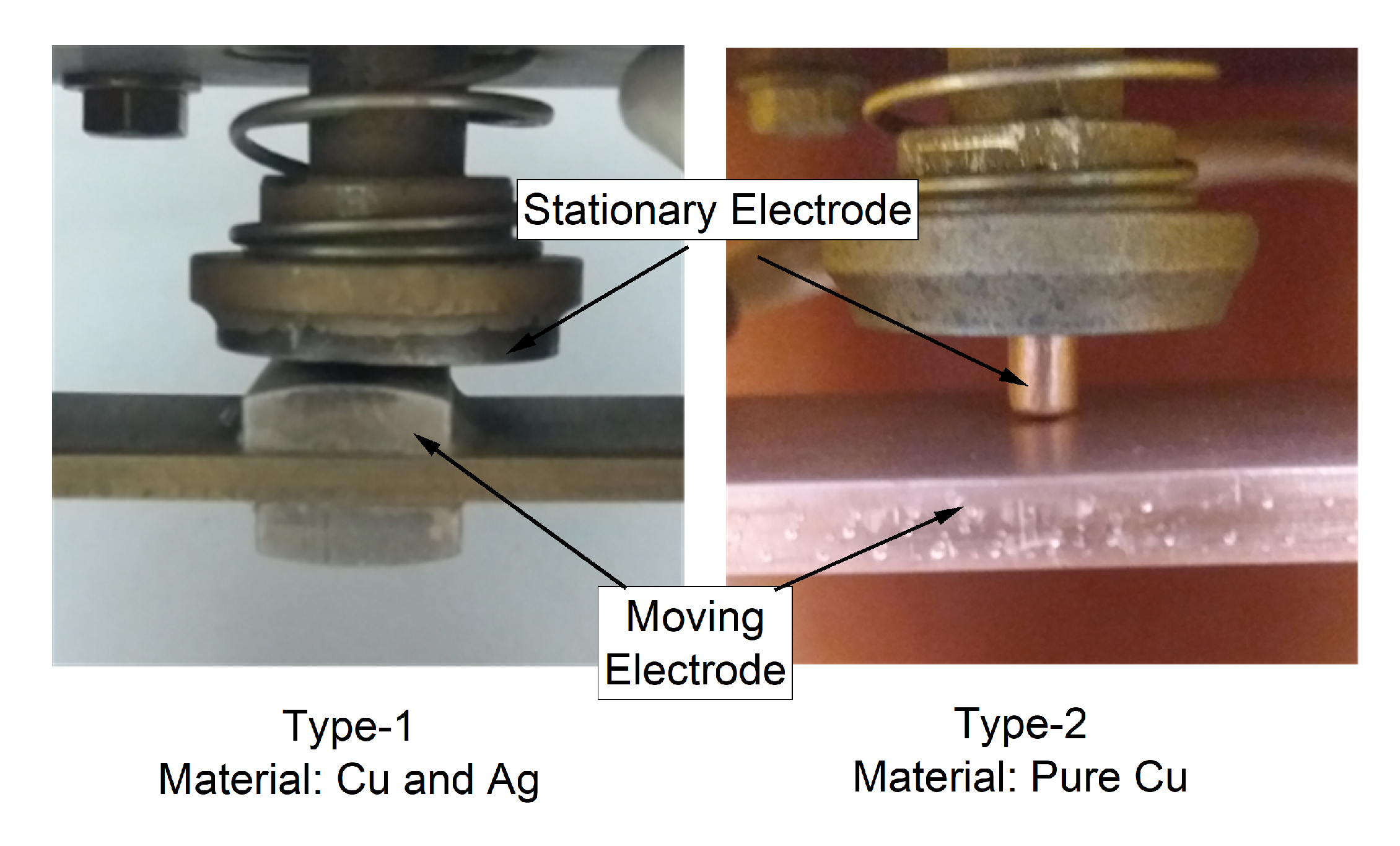
The contact system consists of a normally closed switch with a single set of vertically orientated contacts. The upper contact is stationary and the bottom spring loaded contact is pulled down by a solenoid to open the switch (spring tension is required to maintain a sufficient contact force). Two different contact configurations are used in the experiments, as shown in Figure 1.
The configuration designated as Type-1 is the original unmodified form of an existing switch with metal alloy contacts consisting of mainly copper and silver. The upper electrode of the Type-1 contacts is a round disc with a flat surface of diameter 24 mm; the lower contact electrode is a rectangular prism or cuboid with an arched top 4 mm high, affixed to a 3 mm thick copper plate. The contact pair creates a contact line spanning the diameter of the upper disc.
For comparison and to illustrate the impact of contact material, a second contact configuration designated as Type-2 has been considered. Another alloy is avoided and pure copper contacts are used to allow for future optical studies (copper has very well defined spectral lines, which can be separated from those of gases, i.e., oxygen). In addition, one electrode with a much smaller contact surface was chosen; the upper contact is cylindrical with a slightly domed surface of diameter 4.5 mm; the lower electrode is a 4 mm thick (Cu) plate. This contact pair with a single contact point has been considered to force more symmetric arc behaviour and to limit the complexity, which may support forthcoming studies by physical arc modelling. It should be noted that a comprehensive study of the variety of contact materials and configurations in low-voltage switching are out of the scope of the present study.
Both contact pairs are mounted in identical normally closed solenoid-actuated switches with a maximum gap spacing (fully open) of nearly 33.5 mm. The experiments were performed in open-air at atmospheric pressure and at room temperature.
2.2. Circuit Schematic
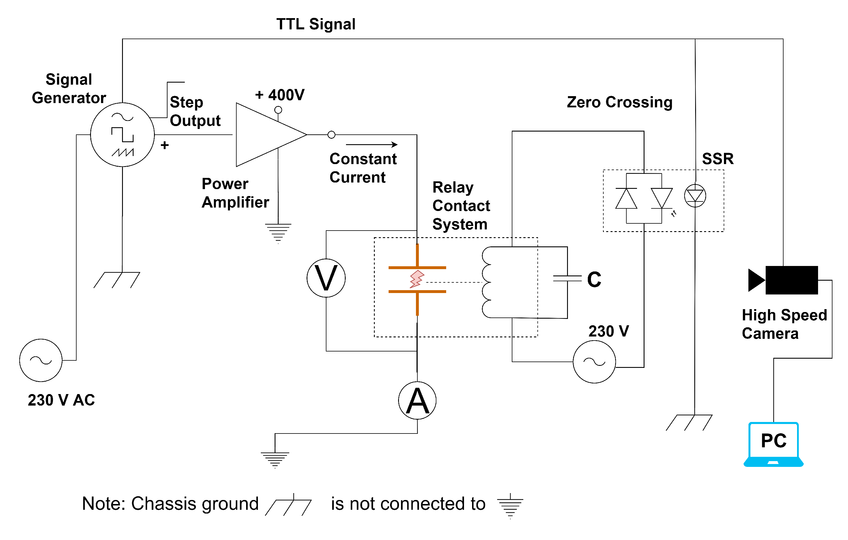
The circuit schematic of the test arrangement is shown in Figure 2, which mainly consists of a power supply (amplifier), a switch (contact system), and a measurement system. The pulsed DC input from the signal generator (Agilent Technologies 33220A) is supplied to the power amplifier (FM1295 from FM Elektronik Berlin) with a BNC connector. The amplifier is used to supply a constant DC current across the switch during the contact separation process. It has a rated output voltage of 400 V RMS and a maximum rated current of 28 A. The voltage and current waveforms across the contacts are measured with a digital oscilloscope (Yokogawa DLM2054) using a passive voltage probe and the built-in shunt of the power amplifier, respectively. The coil of the solenoid-actuated switch is energised with 230 V AC via a solid state relay (SSR), with zero voltage (crossing) switching, to allow repeatable contact separation velocities. The inherent electrical and mechanical delay of the switch actuator gives enough time for the current to settle before the contacts separate. The signal generator is triggered manually, thereby setting the switch current to the desired value by means of the power amplifier; the TTL trigger output, ’SYNC’, in turn actuates the switch via the SSR and the high-speed camera, whereas the oscilloscope is self-triggered by the measured current. A surge suppression capacitor is connected across the coil to eliminate signal interference or noise.
2.3. Optical Setup
A monochromatic high-speed camera (Chronus 1.4 from Kron Technologies) with a spectral range of between 400 and 800 nm [27], is used to record high-speed images of the contact separation arcs. The camera is mounted at a distance of 1 m from the switch during the experiments and is controlled by a computer through an Ethernet cable with an external trigger, using the ‘Trigger End’ and ‘Post-Trigger Images’ mode options to record a predefined number of images (time) after the trigger. A series of arc images from each experiment are thus stored for further processing. The experiments with Type-1 contacts are performed at a relatively higher exposure rate than those with the Type-2 contacts (the complete settings are given in Table 1).
3. Methods and Data Processing
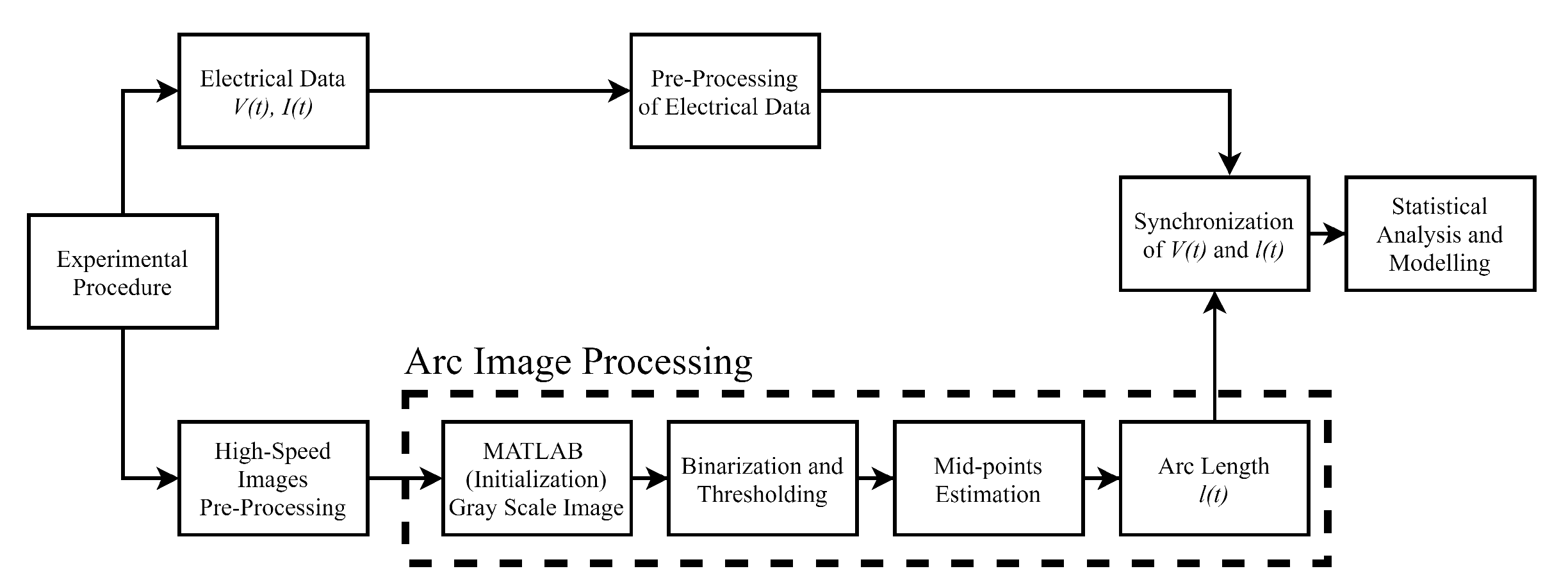
Figure 3 shows the block diagram of the data processing with the two types of data obtained, i.e., electrical data in the form of arc voltage and arc current and optical data in the form of high-speed camera images (HSI). The data are processed and synchronised in MATLAB (Mathworks Inc., Natick, MA, USA) and Origin (OriginLab, Northampton, MA, USA) software programs.
3.1. Electrical Data
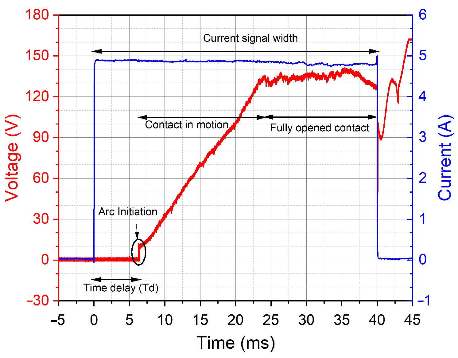
Figure 4 shows a typical waveform of the arc voltage development at a current of 4.87 A. Initially, the electrical contacts are closed, and no electrical current is flowing. The DC voltage signal, that corresponds to a relative current value at the power amplifier, is set on the signal generator and the device is triggered at s to actuate the switch and turn on the current. A constant current starts to flow while the contacts are still closed. After a time delay , caused by the switch actuator and SSR, the contacts start to separate, and the arc voltage sharply rises. With the increase in arc length, the voltage also increases. The arc is sustained even after the contacts have been fully separated and is switched off after the preset time of 40 ms, to reduce the arc burning time and contact erosion. The arc voltage and current is measured for the entire duration of the contact separation at a time resolution of 0.4 . The measured data are analysed in its raw form to determine the initial voltage step and is filtered to reduce signal noise and small artifacts produced by the arc, to determine the time varying slope. A post-process Gaussian filter in MATLAB with a window of 100 data points or 40 is used for the latter.
3.2. High Speed Images Data
An image processing technique is implemented in the MATLAB software to calculate the arc length. The radiation distribution is considered as an indication of the arc shape. It is also assumed that the mean current path coincides with the centre of the arc’s radiation distribution. It is observed that the arc does not follow a straight line and thus has a length greater than the contact gap. Furthermore, the arc length calculation is based on arc images from one viewing angle only, and elongations of the arc in the direction perpendicular to the considered plane must also be expected. Consequently, the arc lengths calculated here is a lower limit of the real arc length and would require tomographic analysis to improve the arc length determination. However, the arc elongation is less pronounced in our experiments (in particular at low gap distances where the arc remains within a fairly straight line).
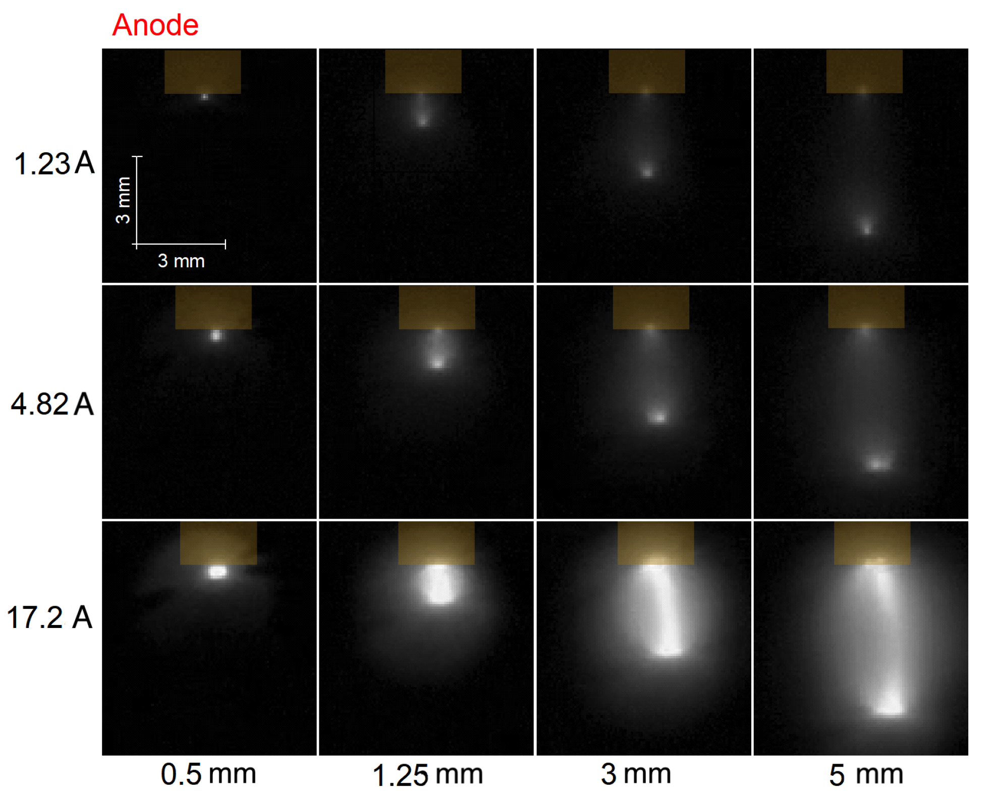
To find the arc length, the path is traced by determining the mid-points for every horizontal cross-section along the entire vertical length of an arc image. The arc image is obtained from the high-speed camera and is imported into MATLAB as an 8-bit grayscale indexed image. Figure 5 shows representative arc images at three current values and different arc lengths for the Type-2 contacts.
3.2.1. Binarization of an Arc Image
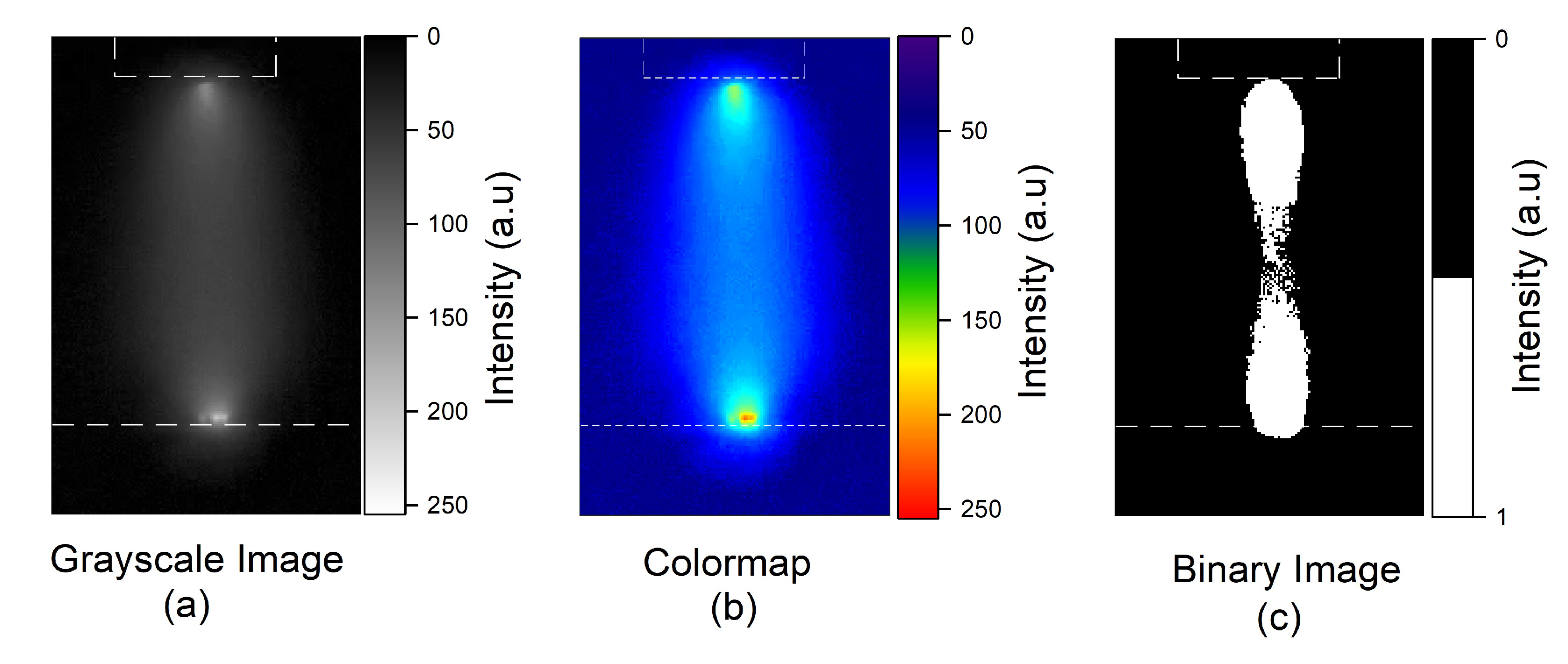
The grayscale image (with pixel intensities 0–255) is converted into a binary image using an appropriate threshold value. This sets the intensity value of x pixel to either maximum ‘1’ or minimum ‘0’. Figure 6 shows the grayscale image (a), its intensity distribution in the colormap (b) and the binary converted image (c) at 8.60 A. The white dashed line indicates the approximate position of contacts. Since, the radiation intensity changes with the arc current and arc length (see Figure 5). This creates a difficulty in making the suitable selection of threshold value. Therefore, various values are checked at multiple positions of the arc, and finally, appropriate values are selected manually for different arc lengths. For arc images with lower length (approximately less than 1.5 mm), the radiation intensity is high in the entire region between contacts. Accordingly, the high threshold value is selected in the range of pixel intensities between 200 and 240. Whereas, arc images at higher lengths exhibits high radiation intensity near contacts and low intensity in the middle part. The high threshold value in this case, does not give information about the arc column or the middle part of the image due to very low intensity. Consequently, this value is adapted according to the lower intense region, which is between pixel intensities of 80 to 120. The edges of binarized images are also smoothed in order to reduce the roughness of edges (see the difference between Figure 6c and Figure 7b).
3.2.2. Arc Length Calculation
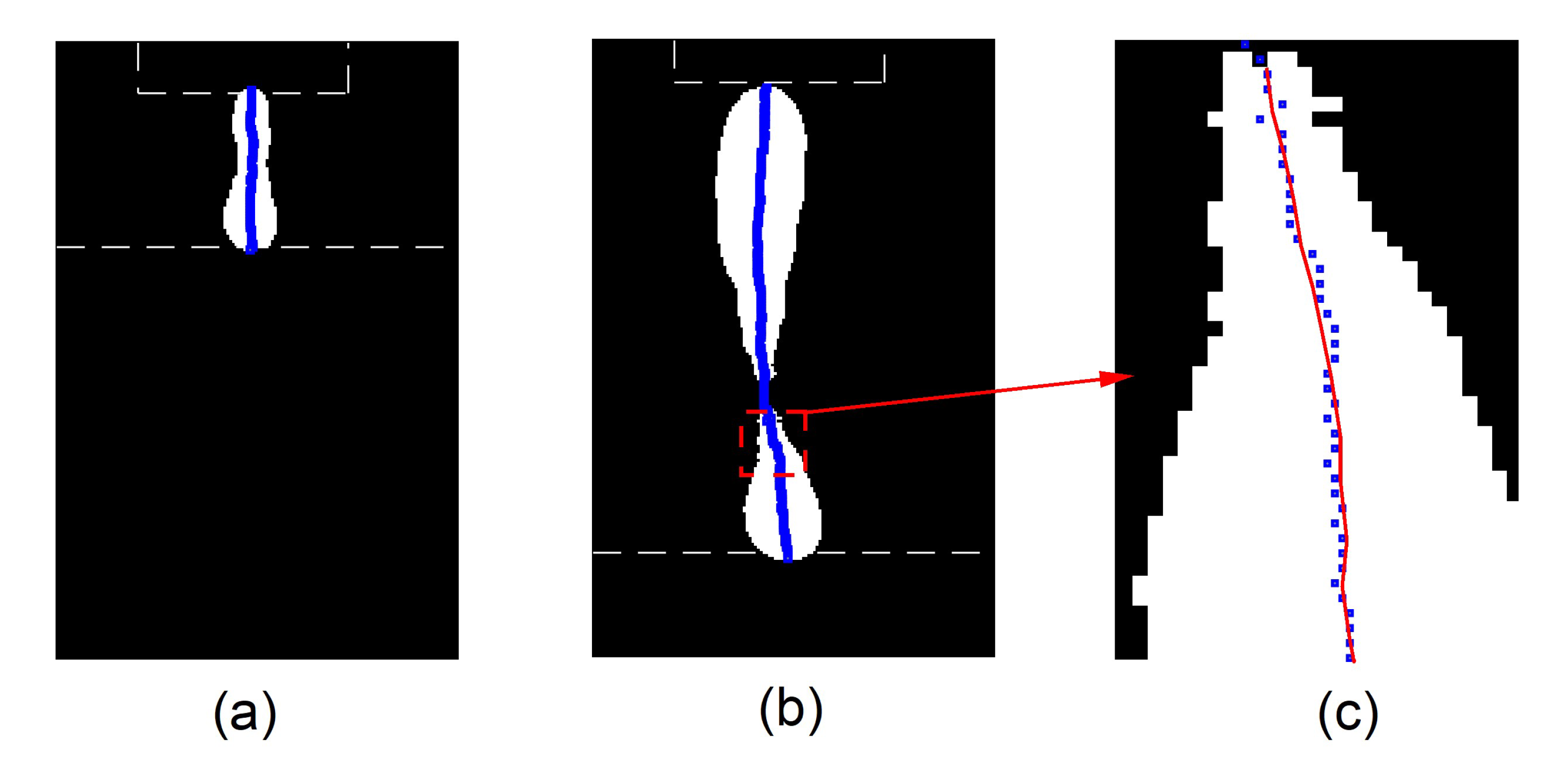
Figure 7 shows the mid-points (blue dots) and the calculated path (red line) along with the magnification for a random binarized image. The white dashed line shows the approximate position of the contacts.
In order to trace this path and estimate the actual length, the arc image is divided into several horizontal slices or small vertical sections. The mid-points are determined at each cross section by finding the (horizontal) median between the first and the last white pixel at every cross-section. The actual length is then estimated by applying a non-linear regression on these mid-points. The arc trace or length development (over time) thus obtained is correlated with the expected contact gap separation determined from an experiment performed without an arc using a high exposure time (where the electrode’s positions were highly visible). The arc images were analysed using various exposure times. Exposure times in the range of 50 to 100 yield an overexposed image and could result in overestimation of arc length. The minimum acquisition time that could be used with this camera was 1 . Therefore, all the results in this paper were obtained from images with 1 exposure time. Finally, the time-domain data of the arc length and arc voltage is synchronised and combined to obtain the voltage vs. distance function, the slope of which represents the electric field. The time between the two consecutive images is much higher than the temporal resolution of electrical data. Therefore, the voltage data points are reduced to match the time of the HSIs.
4. Results
The current-voltage waveforms have been measured and the DC arc images have been observed following the data processing steps for the experimental arrangement shown in Figure 2. The arc voltage and the arc length are considered up to 80 V and 6 mm, respectively. is evaluated at several arc current values between 0.8 and 20 A. In this section, results are compiled for both types of contacts.
4.1. Arc Voltage vs. Time and Initial Arc Voltage
The arc voltage is measured across the switch contacts. A sudden voltage step is observed at the instant of contact separation, which is not synchronised with the trigger pulse, due to the delayed switching of the SSR and the mechanical actuator. Therefore, the time series is shifted so that the onset of the voltage step corresponds to the instant of triggering at s. This is needed so that the optical and electrical data may be compared.
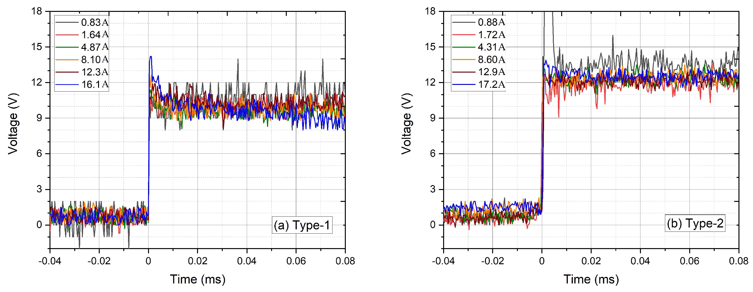
Figure 8 shows the initial arc voltage behaviour after contact separation for various test currents with (a) Type-1 contacts and (b) Type-2 contacts. Note that a Gaussian filter has not been applied to the voltage data shown in Figure 8 (see Section 3.1). The time resolution was not fine enough to measure the voltage step response accurately. However, after a settling time of approximately 20 , the voltage remains fairly constant for at least 40 . The average voltage in the time range t = 0.02–0.06 ms is recorded as the initial arc voltage. The initial arc voltage is between 9 and 11 V for the Type-1 and between 11 and 13 V for the Type-2 contacts. The measured arc voltage waveforms , are given in Figure 9 for (a) Type-1 contacts and (b) Type-2 contacts at several constant currents up to a time of 7 ms.
4.2. Arc Length vs. Time
The arc length is estimated from HSI as described in Section 5. Figure 10 shows the arc length for each experiment at different currents as well as the estimated contact distance , which is obtained from HSI without an arc at higher frame rate and acquisition time. The results show a good correlation between them as is typically slightly greater than . It should be mentioned that at the initial phase of switching, for a very short arc length of up to approximately 0.5 mm, the arc intensity is very low and arc length spans no more than 4 to 5 pixels. As both experiments had slightly different observation distances, each pixel for the Type-1 and Type-2 contacts represent 0.10 and 0.08 mm, respectively. The arc length increases monotonically due to the sinusoidal power supply and the inertia of the solenoid switch armature as well as the action of the spring.
4.3. Arc Voltage as a Function of Arc Length
The arc voltage as a function of the arc length for different currents is shown in Figure 11. The results are obtained after synchronising and comparing the arc voltage data and the arc length data from the HSI. Two positions of interest can be observed. Firstly, an almost instantaneous increase in the voltage is assumed at the instant of contact opening ( mm). Secondly, the approximate value mm is considered as the transition point , where there is a definite change in the voltage gradient. From the analysis of measurement data in Figure 11, it is assumed that the total arc voltage is the sum of two independent linear functions each representing a specific arc region; therefore, the measured data is fitted with a piecewise linear model by considering the three regions:
- Initial arc voltage at time instant of contact opening ();
- Short arc case when the arc length is less than transition value ;
- Long arc case when the arc length is greater than and equal to transition value ().
Mathematically these cases can be described by:
where is the arc length in mm and is the transition point of the electric field, which is fixed at 1.25 mm for model simplification. is the electric field of the arc when and is the electric field in the enlarged arc region of longer arcs with .
4.4. Electric Field
The fit function applied in Figure 11 gives the value of E for both arc regions. The electric field is mathematically defined as
Table 2 shows the fit values of and for both types of electrodes along with the percentage standard error (SE). In order to simplify the model, the value of in (3) and (4) is taken as constant 10 and 12 V for Type-1 and Type-2 contacts, respectively. This has been done for two reasons: no systematic change of with current has been observed, and an error much larger than 2 V would occur in the fit of from a linear regression of the voltages over gap length up to 1.25 mm without fixing.
The resulting electric field E is plotted in Figure 12, for the regions and as a function of arc current for both contact types. The electric field versus the current follows a non-linear decaying exponential function; the decay functions are similar in both arc regions, but are shifted in magnitude. To model the expected electric field of the arc, the estimated field and current data thus obtained is fitted using the following non-linear equation:
where is the resistance coefficient and the current coefficient.
4.5. Proposed Arc Model
Based on the fitting results previously explained in Section 4.3 and Section 4.4, a new arc model is derived as a combination of piecewise linear modelling of the arc voltage dependent on arc length and the non-linear modelling of the electric field dependent on the current. The arc voltage across the contacts is given more generally as a function of current and length as:
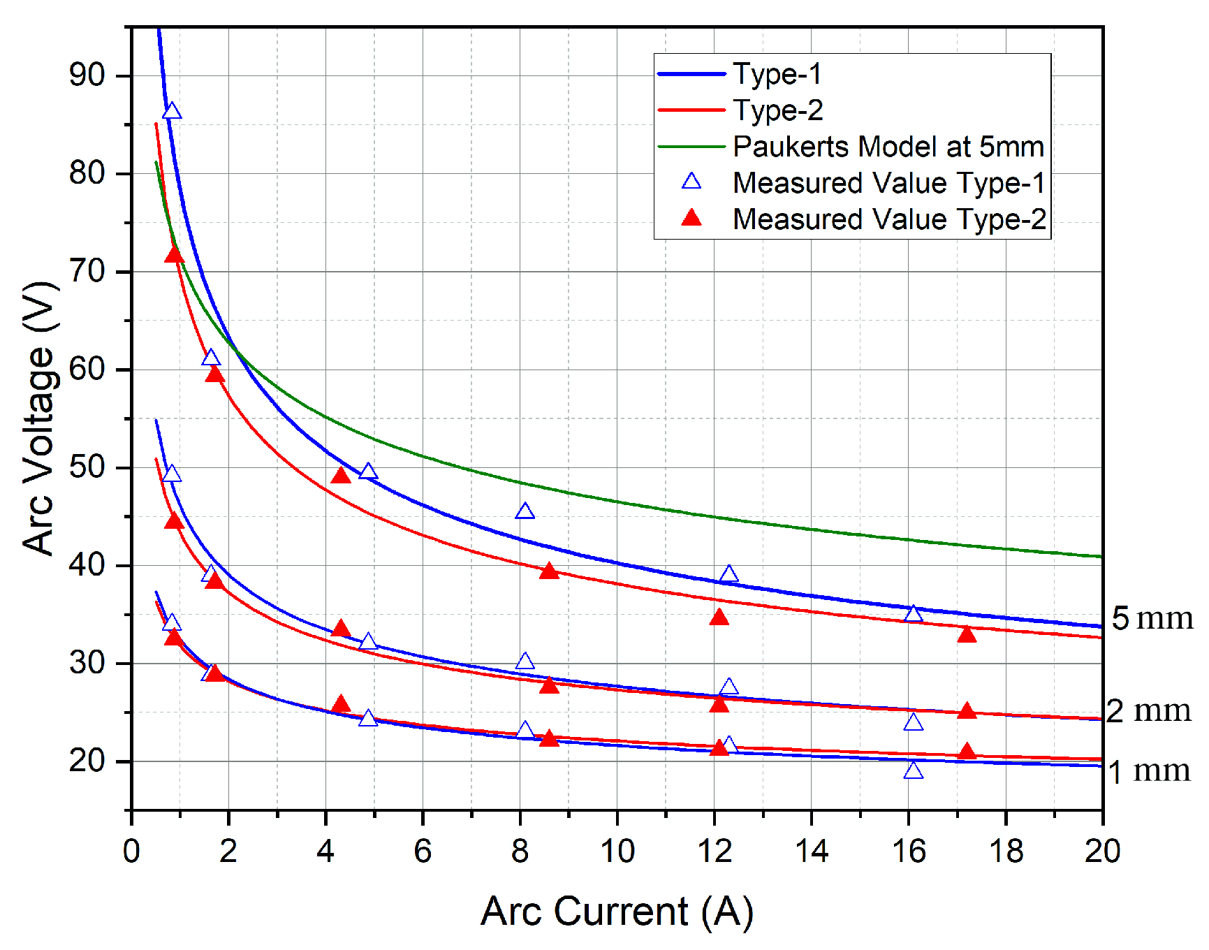
The values of are the fit values according to (5) and given in Table 3 for both contact types. Figure 13 shows the V-I characteristics for various arc lengths from the measurements as well as the corresponding model results according to (6). In addition, the values according to Paukert’s model (1) for the arc length of 5 mm are shown for comparison. The new model matches the measured data better and does not require different equation constants for different arc lengths.
5. Discussion
In what follows, a physical interpretation for the experimental findings will be given. The electrical as well as the optical measurements indicate a clear difference between the behaviour of short and longer arcs. First, the radiation behaviour of short arcs is summarised. At the initial phase of contact opening, the arc shows a low radiation intensity. Instantly after a contact distance of more than 0.3 mm is reached, a bright spot of spherical shape appears. This spot develops to a larger area of intense radiation, which has the approximate shape of a cylinder, terminating at a length of mm. Such an example is shown in the first picture in Figure 14.
In general, an intense radiation is related to a large energy loss in a plasma. Besides the energy consumption caused by the processes of the arc, the arc-electrode interaction has to be taken into account as well (see, e.g., basics of electrode sheath regions in [28]). Energy is required to heat up the cathode for providing sufficient thermal emission of electrons, which may be explained by quantum theory at finite temperatures (thermo field dynamics). Additional energy is required for the acceleration of these electrons, the subsequent gas ionisation needed to establish the plasma and the displacement of accumulated charge (heavy gas ions) in front of the cathode. This charge accumulation is most probably responsible for creating a stable high field region in front of the cathode.
All these energy loss rates must be compensated by the source, which finally results in ohmic heating . It is furthermore expected that the intense radiation as well as the relatively high field strength of the short arc is related to strong deviations from Local Thermodynamic Equilibrium (LTE) in the overall gap area caused by the impact of non-equilibrium processes in the cathode and anode sheath areas.
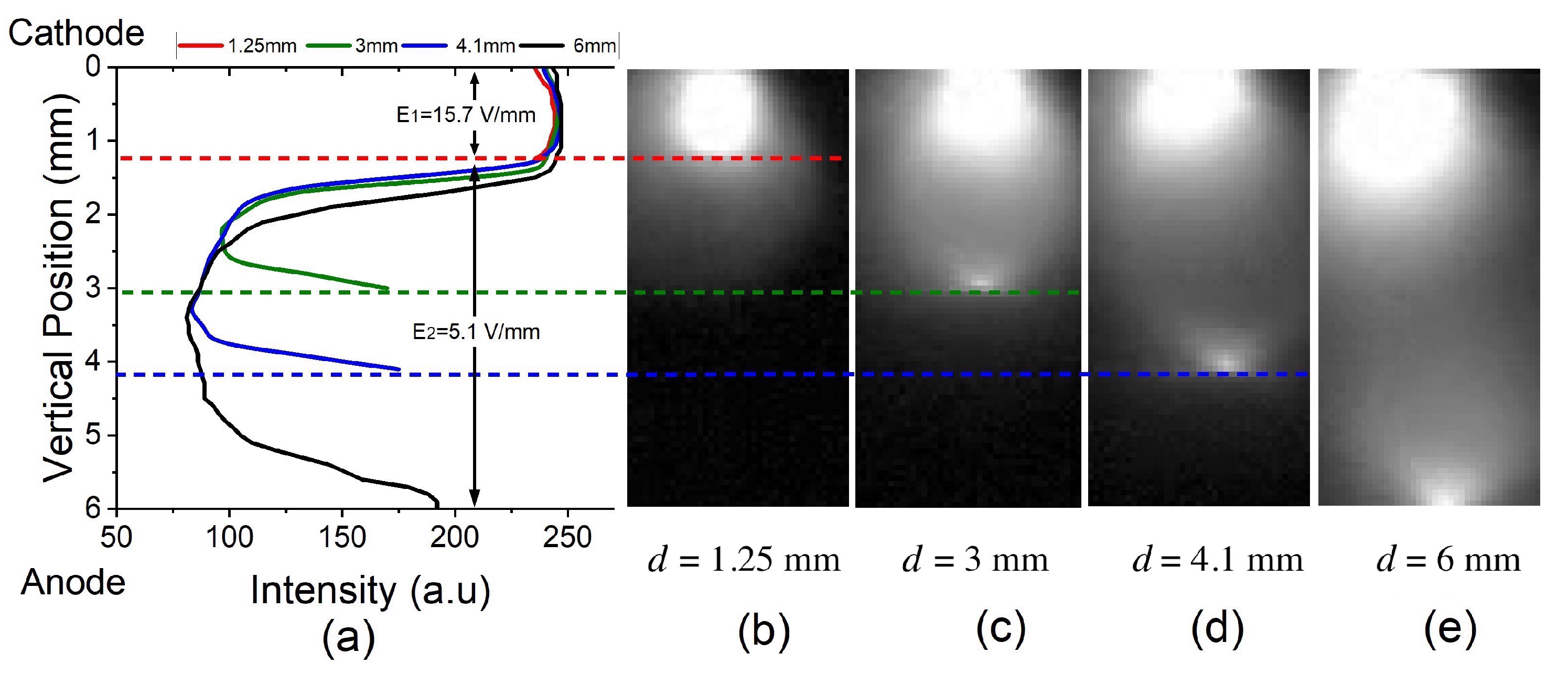
The behaviour changes when the gap distance or the arc length exceeds . Examples are shown in Figure 14b–e. Spots on the anode and cathode separate from each other in longer arcs. Beside the area of intense radiation in front of the cathode of a length of approximately , a small anode spot appears. The region between both spots shows a much lower radiation intensity. Figure 14a shows the maximum intensity for each cross section of the images as the function of the vertical position in the gap. Notice that the curves approximately coincide except of the regions near the anode. The maximum intensity in the darker regions can be lower than in the near cathode area by a factor larger than 3. This is accompanied by low electric field strengths found in the extension area of the arc. An obvious physical interpretation is that the low radiation intensity corresponds to lower energy losses. Consequently, the ohmic heating and the local electric field in the extension area may be lower. It is expected that the arc plasma in such an area is close to LTE and less influenced by the electrode sheath processes.
An additional interpretation for the relatively intense radiation is the occurrence of metal vapour at least in the short arc and in the electrode spots of the long arc. The metal vapour (mostly copper in the present case) would originate from the evaporation of the electrodes in the hot spot regions (see, e.g., [29,30]) and causes strong radiation because of many excitation levels with relatively high transition probabilities and low excitation energies of copper in comparison with the plasma species from the air.
The models for the voltage given in (4) to (6) with the constant coefficients in Table 3 are relatively simple but fit the voltage measurements quite well. Obviously, such models cannot describe temporal voltage fluctuations as shown in Figure 8. The typical SE of fitting results in Figure 11 and Figure 14 is between 1% and 5% also given in Table 2. The maximum SE that occurs is for the estimation of at 0.83 A which is 5.2%. In addition, some deviation from the measured data are caused by fixing the value of . Other errors may come from the arc image analyses due to the spot like radiation at the electrodes and the possibility of miscalculation of arc lengths as a result of the binary conversion process or the choice of intensity threshold values.
Furthermore, the model cannot be used for the description of the detailed voltage behaviour immediately after contact separation in a time scale of microseconds and contact gaps up to 0.3 mm as shown in Figure 9. An investigation of this region was out of the scope of the present work because of limitations of the optical resolution. Beside of the pixel size of 81 in the high-speed imaging, reflection and refraction of the arc light at the electrode surfaces as well as the dynamic behaviour of cathode and anode spots impede a detailed optical analysis. Therefore, the model is applicable in the time scale of 100 and for gap distances above 0.3 mm only.
6. Summary and Outlook
Electrical and optical measurements on a low voltage switch contact system with two different electrode configurations in the range of currents between 0.5 and 20 A have shown a specific behaviour of short arcs up to a length of approximately mm in comparison with longer arcs. Independent of the current and only slightly dependent on the electrode material, a voltage drop between 10 to 13 V appears just after contact separation and can be interpreted as the sum of cathode and anode sheath voltage. Short arcs show intense radiation in the whole gap and a relatively high voltage increase with increasing arc length representing an electric field strength ranging from 9 V/mm for currents A to up to 24 V/mm for currents below 1 A. Such electric fields are much larger than expected in arcs of higher current and indicate strong deviations from LTE.
For larger gap distances and arc lengths above , an arc region of low radiation intensity appears between bright spots at the electrodes. As it was not reported in the literature to our knowledge so far, the bright area with a high voltage gradient of a length of approximately mm remains in front of the cathode almost independent of current and arc length. However, the resulting electric field in the remaining darker arc region above the length is much lower, ranging between 3 V/mm for currents around 20 A and 12 V/mm for currents below 1 A.
Based on the electric measurements, very simple models for the arc voltage dependent on current and arc length are given for both electrode configurations, which fit the experimental measurements quite well. The models are based on the consideration of a constant total sheath voltage, a fixed transition length , where the high electric field changes to a lower value and constant electric fields within each arc region.
The reason for the abrupt change of the voltage slope and the electric field of the arc when its length exceeds as well as a clear interpretation of cannot be given here. Such answers can be probably given by a detailed arc model including the arc-electrode interaction as it has been developed so far only for tungsten inert gas arcs [5,31] adapted for the experimental case. Additional studies, e.g., with optical emission spectroscopy can reveal the role of metal vapour in particular in the short arc and spot regions. Both these studies are out of the scope of the present paper and are planned for future work.
Author Contributions
Conceptualization and methodology, D.U. and P.P.; experimental setup and measurements, A.N. and P.P.; software, A.N.; investigation and formal analysis, A.N.; validation, P.P.; writing—original draft preparation, A.N.; writing—review and editing, P.P. and D.U.; visualization, A.N.; supervision, D.U. All authors have read and agreed to the published version of the manuscript.
Funding
This research received no external funding.
Conflicts of Interest
The authors declare no conflict of interest.
Abbreviations
The following abbreviations are used in this manuscript:
| DC | Direct Current |
| AC | Alternating Current |
| LTE | Local Thermodynamic Equilibrium |
| BNC | Bayonet Neill–Concelman |
| RMS | Root Means Square |
| SSR | Solid State Relay |
| HSI | High Speed Images |
| PC | Personal Computer |
| SE | Standard Error |
References
- Holm, R. Electric Contacts: Theory and Application; Springer: Berlin, Germany, 2013. [Google Scholar]
- Slade, P.G. (Ed.) Electrical Contacts: Principles and Applications; CRC Press: Boca Raton, FL, USA, 2017. [Google Scholar]
- Niayesh, K.; Runde, M. Power Switching Components (Power Systems); Springer: Cham, Switzerland, 2017; ISBN 978-3-319-51459-8. [Google Scholar]
- Rau, S.-H.; Lee, W.-J. DC Arc Model Based on 3-D DC Arc Simulation. IEEE Trans. Ind. Appl. 2016, 52, 5255–5261. [Google Scholar] [CrossRef]
- Siewert, E.; Baeva, M.; Uhrlandt, D. The electric field and voltage of dc tungsten-inert gas arcs and their role in the bidirectional plasma-electrode interaction. J. Phys. D Appl. Phys. 2019, 52, 324006. [Google Scholar] [CrossRef]
- Mayr, O. Beiträge zur Theorie des Statischen und des Dynamischen Lichtbogens. Arch. Elektr. 1943, 37, 588–608. [Google Scholar] [CrossRef]
- Cassie, A.M. Arc Rupture and Circuit Severity: A New Theory. In Proceedings of the Conférence Internationale des Grands Réseaux Électriques à Haute Tension (CIGRE Report), Paris, France, 29 June–8 July 1939; Volume 102, pp. 1–14. [Google Scholar]
- Schavemaker, P.H.; van der Slui, L. An improved Mayr-type arc model based on current-zero measurements [circuit breakers]. IEEE Trans. Power Deliv. 2000, 15, 580–584. [Google Scholar] [CrossRef]
- Habedank, U. Application of a new arc model for the evaluation of short-circuit breaking tests. IEEE Trans. Power Deliv. 1993, 8, 1921–1925. [Google Scholar] [CrossRef]
- Bizjak, G.; Zunko, P.; Povh, D. Combined model of SF/sub 6/circuit breaker for use in digital simulation programs. IEEE Trans. Power Deliv. 2004, 19, 174–180. [Google Scholar] [CrossRef]
- Khakpour, A.; Franke, S.; Gortschakow, S.; Uhrlandt, D.; Methling, R.; Weltmann, K.-D. An Improved Arc Model Based on the Arc Diameter. IEEE Trans. Power Deliv. 2016, 31, 1335–1341. [Google Scholar] [CrossRef]
- Ayrton, H. The Electric Arc; Cambridge University Press: Cambridge, UK, 2012; ISBN 978-1-108-05268-9. [Google Scholar]
- Steinmetz, C.P. Electric power into light, Section VI. The arc. Trans. Am. Inst. Electr. Eng. 1906, 25, 802. [Google Scholar]
- Nottingham, W.B. A new equation for the static characteristic of the normal electric arc. Trans. Am. Inst. Electr. Eng. 1923, 42, 12–19. [Google Scholar] [CrossRef]
- Stokes, A.D.; Oppenlander, W.T. Electric arcs in open air. J. Phys. D Appl. Phys. 1991, 24, 26–35. [Google Scholar] [CrossRef]
- Paukert, J. The arc voltage and the resistance of LV fault arcs. In Proceedings of the 7th International Symposium on Switching Arc Phenomena, Łódź, Poland, 27 September–11 October 1993; pp. 49–51. [Google Scholar]
- Miller, D.; Hildenbrand, J. DC Arc Model Including Circuit Constraints. IEEE Trans. Power Appar. Syst. 1973, 92, 1926–1934. [Google Scholar] [CrossRef]
- Yao, X.; Herrera, L.; Ji, S.; Zou, K.; Wang, J. Characteristic study and time-domain discrete- wavelet-transform based hybrid detection of series DC arc faults. IEEE Trans. Power Electron. 2014, 29, 3103–3115. [Google Scholar] [CrossRef]
- Bauer, E.C.; Niassati, N.; Brothers, J.; Troth, J.; Hensal, J.; Wang, J.; Schweickart, D.; Grosjean, D. Steady State Characterization of Arcing in 540 V DC Distribution Systems; SAE International Technical Paper: Fort Worth, TX, USA, 2017. [Google Scholar] [CrossRef]
- Ammerman, R.F.; Gammon, T.; Sen, P.K.; Nelson, J.P. DC-arc models and incident-energy calculations. IEEE Trans. Ind. Appl. 2010, 46, 1810–1819. [Google Scholar] [CrossRef]
- Lowke, J.J. Simple theory of free-burning arcs. J. Phys. D Appl. Phys. 1979, 12, 1873–1886. [Google Scholar] [CrossRef]
- Andrea, J.; Schweitzer, P.; Carvou, E. Comparison of equations of the VI characteristics of an electric arc in open air. In Proceedings of the 2019 IEEE Holm Conference on Electrical Contacts, Milwaukee, WI, USA, 15–18 September 2019; pp. 76–81. [Google Scholar] [CrossRef]
- Kim, W.; Kim, Y.-J.; Kim, H. Arc Voltage and Current Characteristics in Low-Voltage Direct Current. Energies 2018, 11, 2511. [Google Scholar] [CrossRef] [Green Version]
- Kim, Y.-J. Modeling for Series Arc of DC Circuit Breaker. IEEE Trans. Ind. Appl. 2019, 55, 6. [Google Scholar] [CrossRef]
- Zhang, Z.; Nie, Y.; Lee, W.-J. Approach of Voltage Characteristics Modeling for Medium-Low-Voltage Arc Fault in Short Gaps. IEEE Trans. Ind. Appl. 2019, 55, 2281–2289. [Google Scholar] [CrossRef]
- Beedubail, C.B.; Pieterse, P.; Hoffmann, U.; Uhrlandt, D. Optical and electrical investigation of spark behaviour in DC low-voltage switchgear during contact separation. In VDE High Voltage Technology; ETG Symposium: Berlin, Germany, 2018; pp. 1–5. [Google Scholar]
- User Manual, Chronos 1.4, High Speed Camera. Software Version 0.3.1. Document Revision 5. April 2019. Available online: https://www.krontech.ca/chronos-1-4-resources/ (accessed on 15 October 2020).
- Murphy, A.B.; Uhrlandt, D. Foundations of high-pressure thermal plasmas. Plasma Sources Sci. Technol. 2018, 27, 063001. [Google Scholar] [CrossRef]
- Lins, G. Measurement of the densities of Cu and Ag vapours in a low-voltage switch using the hook method. Appl. Phys. 2012, 45, 205202. [Google Scholar] [CrossRef]
- Franke, S.; Methling, R.; Uhrlandt, D.; Bianchetti, R.; Gati, R.; Schwinne, M. Temperature determination in copper-dominated free-burning arcs. J. Phys. D Appl. Phys. 2014, 47, 015202. [Google Scholar] [CrossRef]
- Baeva, M.; Boretskij, V.; Gonzalez, D.; Methling, R.; Murmantsev, O.; Uhrlandt, D.; Veklich, A. Unified modelling of low-current short-length arcs between copper electrodes. J. Phys. D Appl. Phys. 2020, 54, 025203. [Google Scholar] [CrossRef]
Figure 1.
Two different contact configurations used in experiments.

Figure 2.
Schematic of the circuit arrangement.

Figure 3.
Block diagram of the data processing.

Figure 4.
Typical Volt-Ampere characteristic at 4.87 A.

Figure 5.
High-speed images of an arc at multiple lengths and currents for Type-2 contacts.

Figure 6.
Intensity distribution in a.u (arbitrary unit) of arc image in (a) grayscale image and (b) colormap (c); binary converted image with threshold = 80.
Figure 6.
Intensity distribution in a.u (arbitrary unit) of arc image in (a) grayscale image and (b) colormap (c); binary converted image with threshold = 80.

Figure 7.
Arc length calculation (a) at 2 mm and (b) at 5 mm; (c) magnification of image. Blue dots represent midpoints and red line the calculated path.
Figure 7.
Arc length calculation (a) at 2 mm and (b) at 5 mm; (c) magnification of image. Blue dots represent midpoints and red line the calculated path.

Figure 8.
Arc voltage in the range of contact separation instant for (a) Type-1; (b) Type-2 contacts.
Figure 8.
Arc voltage in the range of contact separation instant for (a) Type-1; (b) Type-2 contacts.

Figure 9.
Arc voltage waveforms at constant currents for 7 ms after contact separation of (a) Type-1 contacts; (b) Type-2 contacts.
Figure 9.
Arc voltage waveforms at constant currents for 7 ms after contact separation of (a) Type-1 contacts; (b) Type-2 contacts.

Figure 10.
Measured arc length with (a) Type-1 contacts; (b) Type-2 contacts.

Figure 11.
Arc voltage as a function of arc length for Type-1 and Type-2 contacts.

Figure 12.
Electric field of the arc regions as a function of arc current.

Figure 13.
V-I characteristics of proposed model.

Figure 14.
(a) Maximum radiation intensity as a function of the vertical position for the Type-1 contacts at an arc current I = 8.1 A; (b) through (e) images of the arc development for different distances or positions d. The dashed lines show the different anode positions for images (b–d) in accordance with the colour legend given above (a) to distinguish the intensity curves for each image.


Table 1.
High-speed camera settings.
| Function | Value |
|---|---|
| Resolution | 400 × 600 pixels |
| Frame rate Type-1 | 179 |
| Frame rate Type-2 | 80 |
| Exposure time | 1 |
| Trigger source | External trigger BNC (IO1) |
| Trigger mode | Trigger end |
Table 2.
Electric field fit values according to (4) for both cases at various currents.
Table 2.
Electric field fit values according to (4) for both cases at various currents.
| Type-1 Contacts | Type-2 Contacts | ||||||||
|---|---|---|---|---|---|---|---|---|---|
(A) | (V/mm) | (%) | (V/mm) | (%) | (A) | (V/mm) | (%) | (V/mm) | (%) |
| 0.83 | 23.98 | 3.19 | 12.33 | 5.22 | 0.88 | 20.51 | 2.20 | 9.05 | 2.56 |
| 1.64 | 18.78 | 2.80 | 7.34 | 4.39 | 1.72 | 16.77 | 1.57 | 7.03 | 1.99 |
| 4.87 | 14.18 | 2.19 | 5.78 | 3.31 | 4.31 | 13.70 | 1.22 | 5.68 | 1.62 |
| 8.10 | 12.99 | 2.96 | 5.09 | 4.60 | 8.60 | 10.14 | 1.36 | 3.88 | 0.97 |
| 12.3 | 12.00 | 1.39 | 3.83 | 2.52 | 12.10 | 9.13 | 0.80 | 2.97 | 1.35 |
| 16.1 | 8.86 | 2.63 | 3.60 | 3.97 | 17.20 | 8.80 | 0.80 | 2.61 | 1.40 |
Table 3.
Fit values of constants in the proposed arc voltage model.
| Type-1 Contacts | Type-2 Contacts | |||
|---|---|---|---|---|
| = 22.42 | = 0.285 | = 19.82 | = 0.293 | |
| = 10.72 | = 0.408 | = 8.74 | = 0.385 | |
Publisher’s Note: MDPI stays neutral with regard to jurisdictional claims in published maps and institutional affiliations. |
© 2020 by the authors. Licensee MDPI, Basel, Switzerland. This article is an open access article distributed under the terms and conditions of the Creative Commons Attribution (CC BY) license (http://creativecommons.org/licenses/by/4.0/).
Share and Cite
MDPI and ACS Style
Najam, A.; Pieterse, P.; Uhrlandt, D. Electrical Modelling of Switching Arcs in a Low Voltage Relay at Low Currents. Energies 2020, 13, 6377. https://doi.org/10.3390/en13236377
AMA Style
Najam A, Pieterse P, Uhrlandt D. Electrical Modelling of Switching Arcs in a Low Voltage Relay at Low Currents. Energies. 2020; 13(23):6377. https://doi.org/10.3390/en13236377
Chicago/Turabian StyleNajam, Ammar, Petrus Pieterse, and Dirk Uhrlandt. 2020. "Electrical Modelling of Switching Arcs in a Low Voltage Relay at Low Currents" Energies 13, no. 23: 6377. https://doi.org/10.3390/en13236377
Note that from the first issue of 2016, this journal uses article numbers instead of page numbers. See further details here.