Numerical Solution of Biomagnetic Power-Law Fluid Flow and Heat Transfer in a Channel

Abstract

The effect of non-Newtonian biomagnetic power-law fluid in a channel undergoing external localised magnetic fields is investigated. The governing equations are derived by considering both effects of Ferrohydrodynamics (FHD) and Magnetohydrodynamics (MHD). These governing equations are difficult to solve due to the inclusion of source term from magnetic equation and the nonlinearity of the power-law model. Numerical scheme of Constrained Interpolation Profile (CIP) is developed to solve the governing equations numerically. Extensive results carried out show that this method is efficient on studying the biomagnetic and non-Newtonian power-law flow. New results show that the inclusion of power-law model affects the vortex formation, skin friction and heat transfer parameter significantly. Regardless of the power-law index, the vortex formation length increases when Magnetic number increases. The effect of this vortex however decreases with the inclusion of power-law where in the shear thinning case, the arising vortex is more pronounced than in the shear thickening case. Furthermore, increasing of power-law index from shear thinning to shear thickening, decreases the wall shear stress and heat transfer parameters. However for high Magnetic number, the wall shear stress and heat transfer parameters increase especially near the location of the magnetic source. The results can be used as a guide on assessing the potential effects of radiofrequency fields (RF) from electromagnetic fields (EMF) exposure on blood vessel.

1. Introduction

Biological fluid such as blood includes protein, cell membrane and, haemoglobin molecules that contribute to its paramagnetic behaviour, while the content of hydrogen, oxygen, nitrogen and carbon atoms in vessel tissues contribute to its diamagnetic property [1,2]. Biofluid that has magnetic characteristics and able to interact with an applied magnetic field is called biomagnetic [3]. When an external magnetic field is imposed on the biomagnetic fluid, there are two body forces acting on the fluid, magnetisation force and Lorentz force. These two forces correspond to the principle of Ferrohydrodinamics (FHD) and Magnetohydrodynamics (MHD) respectively. The interplay between its hydrodynamics and magnetic properties when external magnetic field gradient is applied has been the topic of great interest [4]. Motivation in these studies are driven by the biomedic application such as in magnetic drug targeting in tumor treatment, hyperthermia, reduction of bleeding during surgeries, and magnetic separation of cells [5,6,7,8,9,10,11]. However, at the same time, there are some drawbacks of magnetic fields toward human bodies. Being exposed to electromagnetic field (EMF) have deleterious effects to living organism [12]. In the last decade, over three billions people are exposed to EMF daily from wireless phone, wi-fi, transmitting towers and base stations [13]. Moreover, there are 150 million patients annually used Magnetic Resonance Imaging(MRI) for clinical examinations [14]. Magnetic field intensity from phone, refrigerator, wireless etc are measured up to 1 T (Tesla) [15], while the MRI is at 1.5 T, 3 T, 7 T [16] and about to be boost up to 14 T [17]. The EMF has biological impact on thermal effect occurs via an alteration in temperature from radiofrequency (RF) fields. There is a possibility that every interaction between RF fields and living tissues causes an energy transfer resulting in a rise in temperature [12]. Therefore, more studies need to be done in order to understand the thermal effects associated with RF exposure.

Several existing studies have examined the effect of applying high magnetic field intensity on the cellular components of the biological fluids. Ichioka et al. [18] reported that the static magnetic field of 8 T significantly decreased the skin blood flow and the body temperature in anaesthetised rat. Similar results have been reported by Haik et al. [19] who studied the effect of magnetic field up to 10 T on human blood. They found that the Reynolds number is decreased when the magnetic field is increased. Motta et al. [20] investigated the effect of magnetic field up to 18 T on light absorption of blood and reported that there is an increase on light absorption level due to paramagnetic orientation of heme group. Higashi et al. [21] studied the effect of applying high static magnetic field up to 8 T on the orientation of normal erythrocytes and found that even at 1 T, the magnetic field influenced the erythrocytes to be oriented with their disk plane parallel to the magnetic field direction.

Mathematical model for biomagnetic fluid flow with an external magnetic field has been introduced by Haik et al. [19], where the arising force due to magnetisation depends on the existence of a spatially varying magnetic field and the biofluid is considered to be electrically poor conductors. This mathematical model is known as Biomagnetic Fluid Dynamics (BFD) [22]. Tzirtzilakis and Loukopoulos [2,23,24] extended this model by considering that blood also exhibit strong electrical conductivity which eventually interacts with the magnetic fields when it flows and give rise to Lorentz force. The mathematical model developed for the biofluid flow under the influence of an applied magnetic field is consistent with the principles of FHD and MHD of ferrofluid [25]. In addition, ferrofluid can exhibit non-Newtonian behaviour [26,27,28,29]. However, most of the available works reported only on the effect of FHD on Newtonian fluid [2,23,30,31,32,33,34,35,36,37,38,39,40,41,42,43]. Even if the magnetic field effect is included in power-law fluid flow, the works only used magnetic field effect of MHD [44,45,46,47,48,49]. Research on the magnetic fluid flow undergoing external magnetic field are extensive. For the research specifically on flow in a channel, Loukopoulos and Tzirtzilakis [23] studied the biomagnetic channel flow where the magnetic field is spatially varying linearly with temperature and magnetic intensity and found that a vortex is arising near the lower plate below of which the magnetic source is placed. This vortex increased in the size depending on the magnitude of applied the magnetic field. Goharkhah and Ashjaee [30] reported the works of using alternating nonuniform magnetic field on ferrofluid flow and heat transfer in a channel. The works on uniform localised magnetic field effect in a channel has been studied by Tzirtzilakis and Loukopolous [2] in laminar flow and Tzirtzilakis et al. [31] in turbulent flow. They found that the effect of magnetic field is decreased in the turbulent flow. Siddiqa et al. [32] studied the effect of including thermal radiation on energy equation in the biomagnetic fluid flow in a channel. A great deal of works have been done on the magnetic field undergoing external magnetic field in geometry other than straight channel. Biomagnetic fluid flow in stenosed channel has been studied by Tzirtzilakis [33], Xenos and Tzirtzilakis [34], and Türk et al. [35]. Türk et al. [36] studied the biomagnetic fluid flow in a channel with multiple stenoses. Flow in aneurysm channel has been studied by Tzirtzilakis [37], and recently by Sharifi et al. [38] on drug targeting using magnetic particles. Tzirakis [39] studied biomagnetic fluid flow in circular ducts. For the works on magnetic fluid flow in lid driven cavity, it has been studied by Tzirtzilakis and Xenos [40], Marioni et al. [41], Bozkaya et al. [42] and by Senel and Tezer-Sezgin [43].

However, most of the works mentioned are concerned with biomagnetic of Newtonian fluid. When blood flows through larger arteries, it behaves according to Newtonian model, but in small blood vessels such as narrow arteries, it behaves according to non-Newtonian flow model at low shear rates [50,51,52,53,54]. Unlike Newtonian fluid, non-Newtonian are a broad class of fluid where the relation between the shear rate and shear stress is nonlinear. Hence, no single constitutive equation can be used to single handedly predict all the flow of non-Newtonian models in various condition. There are several models characterizing flow of blood such as Walburn-Schneck, Casson, Carreau-Yasuda, Quemada, and power-law, where each has its own importance in theoretical and experimental of flow phenomena [55,56,57,58,59]. The power-law model is the simplest form and commonly used for modelling shear-thinning or shear-thickening behaviour of non-Newtonian fluids on certain range.

On the study of purely hydrodynamics power-law flow, Bell and Surana [60] investigated the flow of non-Newtonian power-law in lid driven cavity using p-version least squares finite element formulation and provided the benchmark results for shear thinning and shear thickening flow in lid driven cavity. Their results on power-law lid driven cavity were validated by Neofytou [61], who also carried out simulations for Bingham plastics, Casson and Quemada fluid flow. There are many works that have been reported on magnetic field effect on power-law fluid flow. Kefayati [44] studied the effect of MHD magnetic field on power-law in cavity with two-square concentric duct. Kefayati [45] studied the effect of magnetic field on mixed convection on shear thinning fluids in a cavity with sinusoidal boundary conditions. Adıgüzel and Atalık [46] investigated the effect of MHD magnetic field on power-law ferrofluid flow past a circular cylinder. Jahanbakshi [47] reported the MHD magnetic field effects on natural convection using power-law fluid in an L-shaped enclosure. Ikbal et al. [48] and Sankar et al. [49] investigated the effect of MHD magnetic field on power-law in a stenosed artery. All of these works conclude that the vortex formation decreases under the action of MHD magnetic field. A number of investigations reported works on MHD effect on non-Newtonian flow other than power-law model. Misra et al. [62] studied the works of MHD viscoelastic fluid in a channel with stretching walls and reported that increasing the strength of the magnetic field will have the fluid velocity profile decreases but the temperature profile increases. Liu [63] performed an analysis of electrically conducting fluid of second grade in a porous medium over a stretching sheet subject to a transverse magnetic field and found that when the Eckert number is large, the heat flow transferred from the fluid to the wall rather than from the wall to the fluid when Eckert number is small.

The works that combine both biomagnetic and power-law fluid flow has not been investigated. The reason is that the mathematical model of Navier Stokes with FHD and MHD is difficult to solve due to the magnetisation term FHD introduced in the governing equation. This source term can be very large and will result in instability and divergence of the numerical method without the use of a proper technique. Additionally, in contrast to the Newtonian case, the non-Newtonian fluid flow is generally more complicated to be solved due to its complexity contributed from the constitutive equation to the Navier-Stokes equations. This is due to the fact that the effective viscosity diverges to infinite shear rates and zero shear rates for shear thinning and shear thickening fluid. When solving non-Newtonian flow numerically, it may result in significantly time step constraint when explicit schemes are used, and disrupt the solution technique usually used to solve implicitly the viscous terms in the momentum equation [64]. Several methods have been used to solve the problem analogous in this work. Stream function-vorticity finite difference method (FDM) with stretched grid has been used in [33,65]. FDM central difference has also been used in [48]. In [44,45], finite difference lattice Boltzmann method (FDLBM) is used, while in [35,36] finite element method (FEM) has been applied. In [42,43], dual reciprocity boundary element method (DRBEM) has been used. Lattice Boltzmann method (LBM) has been used in [66,67] while control volume finite element method (CVFEM) is applied to solve the flow problem in [68,69,70]. More detailed review of numerical method on solving FHD and MHD problems are given by Rashidi et al. [71].

An explicit CIP (Constrained Interpolation Profile) with FDM scheme was developed in this work. This scheme is a very stable finite difference technique that can solve generalised hyperbolic equations with third order accuracy in space. Unlike the conventional schemes such as Lax Wendroff and Upwind, this scheme approximated the values of the advection term with its spatial derivative by cubic polynomials interpolation and attains high-accuracy by being less diffusive [72]. The CIP method was introduced by T.Yabe et al. [73,74] and has since been used to solve many various problems [75,76,77]. This method can be combined with other methods [78] as well since CIP is efficient in solving the hyperbolic equation.

As far as we know, no previous research has investigated the works on biomagnetic and non-Newtonian fluid flow using CIP scheme. Therefore the aim of this work is to study the extent of using non-Newtonian power-law on biomagnetic flow in terms of heat transfer, skin friction and flow characteristics where the governing equations are solved numerically using CIP scheme. For non-Newtonian power-law fluid, the viscosity ${\overline{\mu }}_a$ is assumed to be a shear dependent fluid given as

$${\overline{\mu }}_a=m{\left(I_2\right)}^{(n-1)/2},$$

(1)

where m is the fluid consistency, $I_2$ is the second invariant of the rate of strain tensor and n is the power-law index. For two-dimensional flow, $I_2$ is defined as

$$\begin{array}{c}\hfill I_2=2\left[{\left(\frac{\partial \overline{u}}{\partial \overline{x}}\right)}^2+{\left(\frac{\partial \overline{v}}{\partial \overline{y}}\right)}^2\right]+{\left(\frac{\partial \overline{u}}{\partial \overline{y}}+\frac{\partial \overline{v}}{\partial \overline{x}}\right)}^2,\end{array}$$

(2)

where $\overline{u}$ is the velocity along $\overline{x}$-coordinate, and $\overline{v}$ is the velocity along $\overline{y}$-coordinate. For values of $n<1$, the viscosity is shear thinning, while for $n>1$, the viscosity is shear thickening and $n=1$ refers to the Newtonian viscosity model where ${\overline{\mu }}_a=m$. Biological fluids have shear thinning properties as blood has a power-law index at $n=0.6$ and synovial fluid has a power-law index at $n=0.2$ [46]. In addition, this study may give valuable information on the thermal and hydrodynamics effects on blood associated with RF exposure.

2. Problem Formulation

The continuity, momentum and energy equations for biomagnetic fluid flow are given as [24,71]

$$\begin{array}{cc}\hfill & \nabla ·\overrightarrow{v}=0,\hfill \end{array}$$

(3)

$$\begin{array}{cc}\hfill & \rho \left(\frac{\partial \overrightarrow{v}}{\partial \overline{t}}+\overrightarrow{v}·\nabla \overrightarrow{v}\right)=-\nabla \overline{p}+\nabla ·\overrightarrow{\tau }+(\overrightarrow{J}\times \overline{B})+{\overline{\mu }}_0(\overline{M}.\nabla )\overline{H},\hfill \end{array}$$

(4)

$$\begin{array}{cc}\hfill & \rho c_p\left({\displaystyle \frac{\partial \overline{T}}{\partial \overline{t}}}+\overrightarrow{v}·\nabla \overline{T}\right)=\kappa {\nabla }^2\overline{T}+\overrightarrow{\tau }·\nabla \overrightarrow{v}-{\overline{\mu }}_0\overline{T}{\displaystyle \frac{\partial \overline{M}}{\partial \overline{T}}}\overrightarrow{v}·\nabla \overline{H}+{\displaystyle \frac{\overrightarrow{J}·\overrightarrow{J}}{\overline{\sigma }}},\hfill \end{array}$$

(5)

where $\overrightarrow{v}$ is the dimensional velocity vector, $\overline{t}$ is the dimensional time, $\rho$ is the fluid density, $\overline{p}$ is the dimensional pressure, $\overrightarrow{\tau }$ is the stress tensor, $\overrightarrow{J}$ is the current density, $\overline{B}$ is the magnetic field, ${\overline{\mu }}_0$ is magnetic permeability, $\overline{H}$ is the magnetic field intensity, $\overline{T}$ is the dimensional temperature, $c_p$ is the specific heat at constant pressure, $\kappa$ is the thermal conductivity, and $\overline{\sigma }$ is the electrical conductivity.

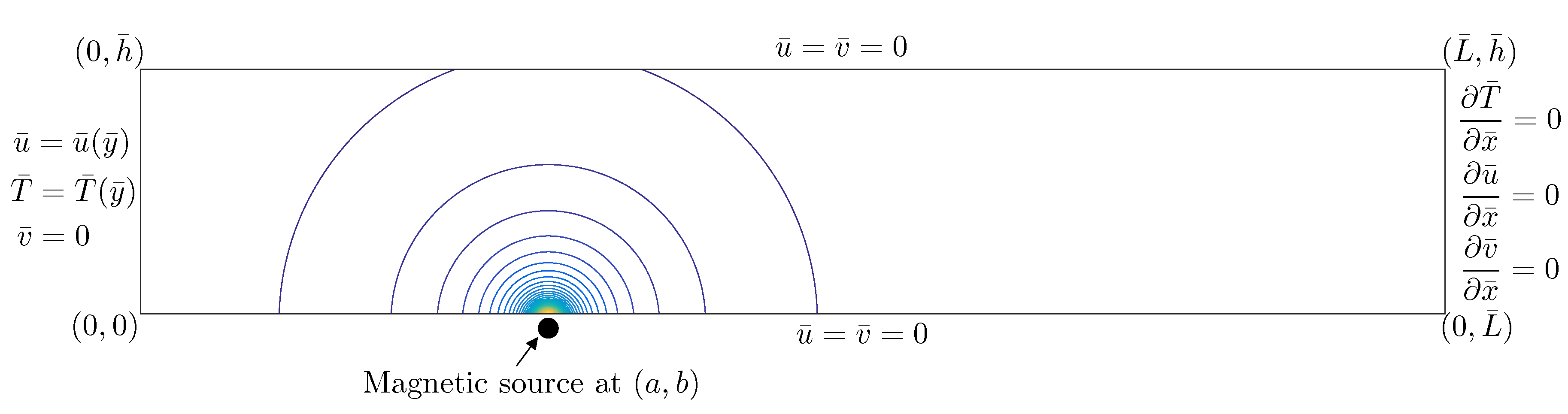
The fluid is considered to be magnetic non-Newtonian and the flow is two-dimensional, laminar, incompressible and under the influence of an applied magnetic field. The body force terms incorporated are from the principles of Magnetohydrodynamics and Ferrohydrodynamics. The flow is considered to be taking place in between two walls. It is assumed that the flow is dominated by the viscous force and the convection is due to temperature gradient, hence the effect of gravity is insignificant. The flow at the entrance is assumed to be fully developed and the walls are kept at a constant temperature ${\overline{T}}_w$, while the fluid is at temperature ${\overline{T}}_f$ such that ${\overline{T}}_w<{\overline{T}}_f$. The configuration of the flow is shown in Figure 1.

With these assumptions, the governing equations in Cartesian form are given as

$$\begin{array}{cc}\hfill \frac{\partial \overline{u}}{\partial \overline{x}}+\frac{\partial \overline{v}}{\partial \overline{y}}& =0,\hfill \end{array}$$

(6)

$$\begin{array}{cc}\hfill \overline{\rho }\left(\frac{\partial \overline{u}}{\partial \overline{t}}+\overline{u}\frac{\partial \overline{u}}{\partial \overline{x}}+\overline{v}\frac{\partial \overline{u}}{\partial \overline{y}}\right)& =-\frac{\partial \overline{p}}{\partial \overline{x}}+{\overline{\mu }}_a\left(\frac{{\partial }^2\overline{u}}{\partial {\overline{x}}^2}+\frac{{\partial }^2\overline{u}}{\partial {\overline{y}}^2}\right)\hfill \\ \hfill & +2\frac{\partial {\overline{\mu }}_a}{\partial \overline{x}}\frac{\partial \overline{u}}{\partial \overline{x}}+\frac{\partial {\overline{\mu }}_a}{\partial \overline{y}}\left(\frac{\partial \overline{v}}{\partial \overline{x}}+\frac{\partial \overline{u}}{\partial \overline{y}}\right)\hfill \\ \hfill & +{\overline{\mu }}_0\overline{M}\frac{\partial \overline{H}}{\partial \overline{x}}-\overline{\sigma }{\overline{B}}_y^2\overline{u}+\overline{\sigma }{\overline{B}}_x{\overline{B}}_y\overline{v},\hfill \end{array}$$

(7)

$$\begin{array}{cc}\hfill \overline{\rho }\left(\frac{\partial \overline{v}}{\partial \overline{t}}+\overline{u}\frac{\partial \overline{v}}{\partial \overline{x}}+\overline{v}\frac{\partial \overline{v}}{\partial \overline{y}}\right)& =-\frac{\partial \overline{p}}{\partial \overline{y}}+{\overline{\mu }}_a\left(\frac{{\partial }^2\overline{v}}{\partial {\overline{x}}^2}+\frac{{\partial }^2\overline{v}}{\partial {\overline{y}}^2}\right)\hfill \\ \hfill & +2\frac{\partial {\overline{\mu }}_a}{\partial \overline{y}}\frac{\partial \overline{v}}{\partial \overline{y}}+\frac{\partial {\overline{\mu }}_a}{\partial \overline{x}}\left(\frac{\partial \overline{v}}{\partial \overline{x}}+\frac{\partial \overline{u}}{\partial \overline{y}}\right)\hfill \\ \hfill & +{\overline{\mu }}_0\overline{M}\frac{\partial \overline{H}}{\partial \overline{y}}-\overline{\sigma }{\overline{B}}_x^2\overline{v}+\overline{\sigma }{\overline{B}}_x{\overline{B}}_y\overline{u},\hfill \end{array}$$

(8)

$$\begin{array}{cc}\hfill \overline{\rho }{c}_p\left(\frac{\partial \overline{T}}{\partial \overline{t}}+\overline{u}\frac{\partial \overline{T}}{\partial \overline{x}}+\overline{v}\frac{\partial \overline{T}}{\partial \overline{y}}\right)& =\kappa \left(\frac{{\partial }^2\overline{T}}{\partial {\overline{x}}^2}+\frac{{\partial }^2\overline{T}}{\partial {\overline{y}}^2}\right)\hfill \\ \hfill & +{\overline{\mu }}_a\left(2\left[{\left(\frac{\partial \overline{u}}{\partial \overline{x}}\right)}^2+{\left(\frac{\partial \overline{v}}{\partial \overline{y}}\right)}^2\right]+{\left[\frac{\partial \overline{u}}{\partial \overline{y}}+\frac{\partial \overline{v}}{\partial \overline{x}}\right]}^2\right)\hfill \\ \hfill & -{\overline{\mu }}_0\overline{T}\frac{\partial \overline{M}}{\partial \overline{T}}\left(\overline{u}\frac{\partial \overline{H}}{\partial \overline{x}}+\overline{v}\frac{\partial \overline{H}}{\partial \overline{y}}\right)+\overline{\sigma }{(\overline{u}{\overline{B}}_y-\overline{v}{\overline{B}}_x)}^2.\hfill \end{array}$$

(9)

In the above equations, $\overrightarrow{v}=(\overline{u},\overline{v})$ is the velocity, $\overline{p}$ is the pressure, $\overline{T}$ is the temperature, $\overline{u}\left(\overline{y}\right)$ and $\overline{T}\left(\overline{y}\right)$ is the parabolic velocity profile and temperature profile respectively for fully developed flow, $\overline{\sigma }$ is the electrical conductivity, ${\overline{\mu }}_0$ is the magnetic permeability vacuum, $c_p$ is the specific heat at constant pressure, $\kappa$ is the thermal conductivity, $\overline{H}=({\overline{H}}_x,{\overline{H}}_y)$ is the magnetic field strength, $\overline{M}$ represents the magnetisation, and $\overline{B}$ is the magnetic induction where $\overline{B}={\overline{\mu }}_0\overline{H}\Rightarrow ({\overline{B}}_x,{\overline{B}}_y)={\mu }_0({\overline{H}}_x,{\overline{H}}_y)$. The bar symbol on $u,v,T,t,x$ and y denote the dimensional form of these quantities.

The components of magnetic field intensity ${\overline{H}}_x$ and ${\overline{H}}_y$ along the $\overline{x}$ and $\overline{y}$ coordinates $\overrightarrow{H}=({\overline{H}}_x,{\overline{H}}_y)$ are given by [40]

$$\begin{array}{c}\hfill {\overline{H}}_x(\overline{x},\overline{y})=\frac{\gamma }{2\pi }\frac{\overline{x}-a}{\sqrt{{(\overline{x}-a)}^2+{(\overline{y}-b)}^2}},{\overline{H}}_y(\overline{x},\overline{y})=-\frac{\gamma }{2\pi }\frac{\overline{y}-b}{\sqrt{{(\overline{x}-a)}^2+{(\overline{y}-b)}^2}},\end{array}$$

(10)

and the magnitude $\overline{H}$ is given by

$$\begin{array}{c}\hfill \overline{H}(\overline{x},\overline{y})=\sqrt{{\overline{H}}_x^2+{\overline{H}}_y^2}=\frac{\gamma }{2\pi }\frac{1}{\sqrt{{(\overline{x}-a)}^2+{(\overline{y}-b)}^2}},\end{array}$$

(11)

where $\gamma$ is the magnetic field strength at the coordinate point of $(a,b)$ where the magnetic source is located. In the magnetic force terms, magnetisation and magnetic field intensity $\overline{H}$ derived experimentally and is given as

$$\begin{array}{c}\hfill \overline{M}=\overline{K}\overline{H}({\overline{T}}_c-\overline{T}),\end{array}$$

(12)

where $\overline{K}$ is a constant and ${\overline{T}}_c$ is the Curie temperature.

The terms ${\displaystyle {\overline{\mu }}_0\overline{M}\frac{\partial \overline{H}}{\partial \overline{x}}}$ and ${\displaystyle {\overline{\mu }}_0\overline{M}\frac{\partial \overline{H}}{\partial \overline{y}}}$ in Equations (7) and (8) respectively represent the component of magnetic force per unit volume and dependent on the existence of magnetic gradient. The term ${\displaystyle {\overline{\mu }}_0\overline{T}\frac{\partial \overline{M}}{\partial \overline{t}}\left(u\frac{\partial \overline{H}}{\partial \overline{x}}+v\frac{\partial \overline{H}}{\partial \overline{y}}\right)}$ in Equation (9) refers to the thermal power unit per unit volume due to the magnetocaloric effect. These three terms arise due to the principles of FHD. The terms $\overline{\sigma }{\overline{B}}_y^2\overline{u}+\overline{\sigma }{\overline{B}}_x{\overline{B}}_y\overline{v}$ and $\overline{\sigma }{\overline{B}}_x^2\overline{v}+\overline{\sigma }{\overline{B}}_x{\overline{B}}_y\overline{u}$ in Equations (7) and (8) respectively represent the Lorentz force per unit volume and included due to the electrical conductivity of the fluid. The term $\overline{\sigma }{(\overline{u}{\overline{B}}_y-\overline{v}{\overline{B}}_x)}^2$ in Equation (9) represents the Joule heating. These three terms arise due to the principles of MHD. Therefore the principle of FHD and MHD are combined in the mathematical model with the application of non-Newtonian fluid.

The non-Newtonian fluid considered here can be represented by the Oswald-de Waele power-law model. The relationship between velocity field and shear stress may be expressed in terms of the effective viscosity as

$$\begin{array}{c}\hfill {\overline{\mu }}_a=m{\left(2\left[{\left(\frac{\partial \overline{u}}{\partial \overline{x}}\right)}^2+{\left(\frac{\partial \overline{v}}{\partial \overline{y}}\right)}^2\right]+{\left[\frac{\partial \overline{u}}{\partial \overline{y}}+\frac{\partial \overline{v}}{\partial \overline{x}}\right]}^2\right)}^{\frac{n-1}{2}},\end{array}$$

(13)

where m is the fluid consistency and n is the power-law index.

The boundary conditions of the problem are

$$\begin{array}{cc}\hfill \mathrm{Inflow}& \overline{u}(0,\overline{y})=\overline{u}\left(\overline{y}\right),\overline{v}(0,\overline{y})=0,\overline{T}=\overline{T}\left(y\right),\hfill \\ \hfill \mathrm{Outflow}& \frac{\partial \overline{u}(\overline{L},\overline{y})}{\partial \overline{x}}=0,\frac{\partial \overline{v}(\overline{L},\overline{y})}{\partial \overline{x}}=0,\frac{\partial \overline{T}(\overline{L},\overline{y})}{\partial \overline{x}}=0,\hfill \\ \hfill \mathrm{Lower}\mathrm{wall}& \overline{u}(\overline{x},0)=0,\overline{v}(\overline{x},0)=0,\overline{T}(\overline{x},0)={\overline{T}}_w,\hfill \\ \hfill \mathrm{Upper}\mathrm{wall}& \overline{u}(\overline{x},\overline{h})=0,\overline{v}(\overline{x},\overline{h})=0,\overline{T}(\overline{x},h)={\overline{T}}_w.\hfill \end{array}$$

(14)

3. Numerical Formulation and Solution Procedure

3.1. Non-Dimensionalisation and Transformation to Stream Function-Vorticity

Equations (7)–(9), with the boundary conditions of Equation (14) are transformed into dimensionless form using the following dimensionless variables

$$\begin{array}{cc}\hfill & x=\frac{\overline{x}}{\overline{L}},y=\frac{\overline{y}}{\overline{L}},t=\frac{\overline{t}\overline{u}}{\overline{L}}u=\frac{\overline{u}}{{\overline{u}}_r},v=\frac{\overline{v}}{{\overline{u}}_r},\hfill \\ \hfill & p=\frac{\overline{p}}{\overline{\rho }{\overline{u}}_r^2},H_x=\frac{{\overline{H}}_x}{{\overline{H}}_0},H_y=\frac{{\overline{H}}_y}{{\overline{H}}_0},{\mu }_a=\frac{{\overline{\mu }}_a{L}^{n-1}}{m{u}_r^{n-1}},T=\frac{\overline{T}-{\overline{T}}_w}{{\overline{T}}_f-{\overline{T}}_w},\hfill \end{array}$$

(15)

where ${\overline{H}}_0=\overline{H}(a,0)$ and $u_r$ is the maximum velocity at the inflow.

To solve the governing equation, stream function-vorticity approach is used and the velocity $\overrightarrow{v}=(u,v)$ is transformed into dimensionless stream function $\psi (x,y)$ and vorticity $w(x,y)$ by the relation

$$\begin{array}{cc}\hfill w& =\frac{\partial v}{\partial x}-\frac{\partial u}{\partial y},\hfill \end{array}$$

(16)

$$\begin{array}{cc}\hfill u& =\frac{\partial \psi }{\partial y},v=-\frac{\partial \psi }{\partial x}.\hfill \end{array}$$

(17)

Using these transformation, the pressure p is eliminated, and Equation (6) is automatically satisfied and hence only the nondimensional variables $\psi$, w and T need to be solved numerically. The transformation results to the following system of equations

$$\begin{array}{cc}\hfill & \frac{{\partial }^2\psi }{\partial x^2}+\frac{{\partial }^2\psi }{\partial y^2}=-w,\hfill \end{array}$$

(18)

$$\begin{array}{cc}\hfill \frac{\partial w}{\partial t}+u\frac{\partial w}{\partial x}+v\frac{\partial w}{\partial y}& =\frac{{\mu }_a}{Re}\left(\frac{{\partial }^{2}w}{\partial x^2}+\frac{{\partial }^{2}w}{\partial y^2}\right)+\frac{1}{Re}\left(\frac{{\partial }^2{\mu }_a}{\partial x^2}-\frac{{\partial }^2{\mu }_a}{\partial y^2}\right)\left(\frac{\partial v}{\partial x}+\frac{\partial u}{\partial y}\right)\hfill \\ \hfill & -\frac{2}{Re}\frac{{\partial }^2{\mu }_a}{\partial x\partial y}\left(\frac{\partial u}{\partial x}-\frac{\partial v}{\partial y}\right)+\frac{2}{Re}\left(\frac{\partial {\mu }_a}{\partial x}\frac{\partial w}{\partial x}+\frac{\partial {\mu }_a}{\partial y}\frac{\partial w}{\partial y}\right)\hfill \\ \hfill & +M{n}_F\left(\frac{\partial H}{\partial x}\frac{\partial T}{\partial y}-\frac{\partial H}{\partial y}\frac{\partial T}{\partial x}\right)\hfill \\ \hfill & +N\left(\frac{\partial }{\partial y}(H_y^{2}u-H_x{H}_{y}v)-\frac{\partial }{\partial x}(H_x^{2}v-H_x{H}_{y}u)\right),\hfill \end{array}$$

(19)

$$\begin{array}{cc}\hfill \frac{\partial T}{\partial t}+u\frac{\partial T}{\partial x}+v\frac{\partial T}{\partial y}& =\frac{1}{RePr}\left(\frac{{\partial }^{2}T}{\partial x^2}+\frac{{\partial }^{2}T}{\partial y^2}\right)\hfill \\ \hfill & +\frac{Ec{\mu }_a}{Re}\left(2\left[{\left(\frac{\partial u}{\partial x}\right)}^2+{\left(\frac{\partial v}{\partial y}\right)}^2\right]+{\left[\frac{\partial u}{\partial y}+\frac{\partial v}{\partial x}\right]}^2\right)\hfill \\ \hfill & +M{n}_{F}EcH(ϵ+T)\left(u\frac{\partial H}{\partial x}+v\frac{\partial H}{\partial y}\right)\hfill \\ \hfill & +EcN{(u{H}_x-v{H}_y)}^2.\hfill \end{array}$$

(20)

The effective viscosity is nondimensionalised to be

$$\begin{array}{c}\hfill {\mu }_a={\left(2\left[{\left(\frac{\partial u}{\partial x}\right)}^2+{\left(\frac{\partial v}{\partial y}\right)}^2\right]+{\left[\frac{\partial u}{\partial y}+\frac{\partial v}{\partial x}\right]}^2\right)}^{\frac{n-1}{2}}.\end{array}$$

(21)

The magnetic field intensity is also nondimensionalised by using Equation (15) and is given by

$$\begin{array}{c}\hfill H(x,y)=\frac{b}{\sqrt{{(x-a)}^2+{(y-b)}^2}}.\end{array}$$

(22)

The boundary configuration for the flow problem is also nondimensionalised using Equation (15) where the length of the horizontal wall is considered to be 10 times the length of the vertical inlet and outlet. The boundary conditions are non-dimensionalised and transformed according to Equations (16) and (17), and given as

$$\begin{array}{cc}\hfill \mathrm{Inflow}& (x=0,0\le y\le 1),\psi =2y^2-\frac{4}{3}{y}^3,w=8y-4,T=4y(1-y),\hfill \\ \hfill \mathrm{Outflow}& (x=10,0\le y\le 1)\frac{\partial \psi }{\partial x}=\frac{\partial w}{\partial x}=\frac{\partial T}{\partial x}=0,\hfill \\ \hfill \mathrm{Lower}\mathrm{wall}& (y=0,0\le x\le 10)\psi =\frac{2}{3},-w=\frac{{\partial }^2\psi }{\partial y^2},T=0,\hfill \\ \hfill \mathrm{Upper}\mathrm{wall}& (y=1,0\le x\le 10)\psi =0,-w=\frac{{\partial }^2\psi }{\partial y^2},T=0.\hfill \end{array}$$

(23)

3.2. Constrained Interpolated Profile (CIP) Based Finite Difference Method

To solve Equations (18)–(23) numerically, the Constrained Interpolated Profile (CIP) method is implemented. In this method, a cubic polynomial is used to interpolate the spatial profile of the value f and its spatial derivative $\nabla f.$ In this case, f is $f=(w,T)$. Once the values of f and $\nabla f$ are calculated, the same values for the next time step are simply obtained by shifting the cubic polynomial.

To implement the CIP algorithm, the governing equations of Equations (19) and (20) are split into two categories [79] which are non-advection phase and advection phase.

Advection Phase:

$$\begin{array}{cc}\hfill \frac{\partial w}{\partial t}+u\frac{\partial w}{\partial x}+v\frac{\partial w}{\partial y}& =0,\hfill \end{array}$$

(24)

$$\begin{array}{cc}\hfill \frac{\partial T}{\partial t}+u\frac{\partial T}{\partial x}+v\frac{\partial T}{\partial y}& =0.\hfill \end{array}$$

(25)

Non-advection Phase:

$$\begin{array}{cc}\hfill \frac{\partial w^{*}}{\partial t}& =\frac{{\mu }_a}{Re}\left(\frac{{\partial }^{2}w}{\partial x^2}+\frac{{\partial }^{2}w}{\partial y^2}\right)+\frac{1}{Re}\left(\frac{{\partial }^2{\mu }_a}{\partial x^2}-\frac{{\partial }^2{\mu }_a}{\partial y^2}\right)\left(\frac{\partial v}{\partial x}+\frac{\partial u}{\partial y}\right)\hfill \\ \hfill & -\frac{2}{Re}\frac{{\partial }^2{\mu }_a}{\partial x\partial y}\left(\frac{\partial u}{\partial x}-\frac{\partial v}{\partial y}\right)+\frac{2}{Re}\left(\frac{\partial {\mu }_a}{\partial x}\frac{\partial w}{\partial x}+\frac{\partial {\mu }_a}{\partial y}\frac{\partial w}{\partial y}\right)\hfill \\ \hfill & +M{n}_F\left(\frac{\partial H}{\partial x}\frac{\partial T}{\partial y}-\frac{\partial H}{\partial y}\frac{\partial T}{\partial x}\right)\hfill \\ \hfill & +N\left(\frac{\partial }{\partial y}(H_y^{2}u-H_x{H}_{y}v)-\frac{\partial }{\partial x}(H_x^{2}v-H_x{H}_{y}u)\right),\hfill \end{array}$$

(26)

$$\begin{array}{cc}\hfill \frac{\partial T^{*}}{\partial t}& =\frac{1}{RePr}\left(\frac{{\partial }^{2}T}{\partial x^2}+\frac{{\partial }^{2}T}{\partial y^2}\right)\hfill \\ \hfill & +\frac{Ec{\mu }_a}{Re}\left(2\left[{\left(\frac{\partial u}{\partial x}\right)}^2+{\left(\frac{\partial v}{\partial y}\right)}^2\right]+{\left[\frac{\partial u}{\partial y}+\frac{\partial v}{\partial x}\right]}^2\right)\hfill \\ \hfill & +M{n}_{F}EcH(ϵ+T)\left(u\frac{\partial H}{\partial x}+v\frac{\partial H}{\partial y}\right)\hfill \\ \hfill & +EcN{(u{H}_x-v{H}_y)}^2.\hfill \end{array}$$

(27)

The computation of advection phase, Equations (24) and (25) is conducted by the CIP method while the non-advection phase, labeled with superscript (*) is solved numerically using finite difference method. In order to adopt this method, the Poisson equation of Equation (18) need to be solved first, then followed by the non-advection phase and finally the advection phase.

Equation (18) is solved by using Successive Overrelaxation (SOR). The iterative procedure is carried out until the residue between two consecutive iteration converges to desired tolerance. The tolerance for SOR is suggested to be smaller than the tolerance for the steady state solution in which $|{\psi }^{new}-{\psi }^{old}|<{10}^{-7}$, and the relaxation factor used is $1.7$.

For the non-advection phase, the explicit scheme is used. The central finite difference discretisation is implemented on first order and second order spatial derivatives terms. The magnetic terms ${\displaystyle \frac{\partial H}{\partial x}}$, ${\displaystyle \frac{\partial H}{\partial y}}$, $H_x$ and $H_y$ are computed analytically from Equation (22). It should be noted that the method has also been tested to be solved using Crank-Nicolson scheme and no significant difference is observed. However using the implicit scheme will require solving the two matrices equation in every time step for each Equations (19) and (20), and inadvertently it is time consuming due to exhaustive computer power required.

Once the non-advection phase are computed, the spatial derivative are calculated for both $w^{*}$ and $T^{*}$. Hence by denoting $f=(w^{*},T^{*})$, the spatial derivative ${{\displaystyle \frac{\partial f}{\partial x}}}^{*}={\partial }_x{f}^{*}$ and ${{\displaystyle \frac{\partial f}{\partial x}}}^{*}={\partial }_y{f}^{*}$ can be calculated as

$$\begin{array}{cc}\hfill {\displaystyle \frac{{\partial }_x{f}_{i,j}^{*}-{\partial }_x{f}_{i,j}^k}{\Delta t}}& ={\displaystyle \frac{f_{i+1,j}^{*}-f_{i-1,j}^{*}}{2\Delta x}}-{\displaystyle \frac{f_{i+1,j}^k-f_{i-1,j}^k}{2\Delta x}}\hfill \\ \hfill & -{\displaystyle \frac{u_{i+1,j}-u_{i-1,j}}{2\Delta x}}·{\partial }_x{f}_{i,j}^k-{\displaystyle \frac{v_{i+1,j}-v_{i-1,j}}{2\Delta x}}·{\partial }_y{f}_{i,j}^k,\hfill \end{array}$$

(28)

$$\begin{array}{cc}\hfill {\displaystyle \frac{{\partial }_y{f}_{i,j}^{*}-{\partial }_y{f}_{i,j}^k}{\Delta t}}& ={\displaystyle \frac{f_{i,j+1}^{*}-f_{i,j-1}^{*}}{2\Delta y}}-{\displaystyle \frac{f_{i,j+1}^k-f_{i,j-1}^k}{2\Delta y}}\hfill \\ \hfill & -{\displaystyle \frac{u_{i,j+1}-u_{i,j-1}}{2\Delta y}}·{\partial }_x{f}_{i,j}^k-{\displaystyle \frac{v_{i,j+1}-v_{i,j-1}}{2\Delta y}}·{\partial }_y{f}_{i,j}^k.\hfill \end{array}$$

(29)

The terms $f^k$, ${\partial }_x{f}_{i,j}^k$, and ${\partial }_y{f}_{i,j}^k$ refer to the values of previous time step. The spatial derivatives of u and v in Equations (28) and (29) are approximated by using central order finite difference.

Once $f^{*}=(w^{*},T^{*})$ and their respective spatial derivative are obtained, they will be used in CIP algorithm. Hence $f^{k+1}=(w^{k+1},T^{k+1})$ are advanced to the new time level after the interpolation of CIP via shifting such that $f^{k+1}=f(x_i-u\Delta t,y_j-v\Delta t)$. Similarly in non-advection phase, the spatial gradient for the new time iteration is also required. The CIP scheme to solve Equation (24) and (25) is given as

$$\begin{array}{cc}\hfill f_{i,j}^{k+1}=& C_{30}\Delta x^3+C_{20}\Delta x^2+{\displaystyle \frac{\partial f_{i,j}^{*}}{\partial x}}\Delta x+f_{i,j}^{*}+C_{03}\Delta y^3+C_{02}\Delta y^2\hfill \\ \hfill & +{\displaystyle \frac{\partial f^{*}}{\partial y}}\Delta y+C_{21}\Delta x^2\Delta y+C_{12}\Delta x\Delta y^2+C_{11}\Delta x\Delta y,\hfill \end{array}$$

(30)

$$\begin{array}{cc}\hfill {\displaystyle \frac{\partial f_{i,j}^{k+1}}{\partial x}}& =3C_{30}\Delta x^2+2C_{20}\Delta x+{\displaystyle \frac{\partial f_{i,j}^{*}}{\partial x}}+2C_{21}\Delta x\Delta y+C_{12}\Delta y^2+C_{11}\Delta y,\hfill \end{array}$$

(31)

$$\begin{array}{cc}\hfill {\displaystyle \frac{\partial f_{i,j}^{k+1}}{\partial y}}& =3C_{03}\Delta y^2+2C_{02}\Delta y+{\displaystyle \frac{\partial f^{*}}{\partial y}}+C_{21}\Delta x^2+2C_{12}\Delta x\Delta y+C_{11}\Delta x.\hfill \end{array}$$

(32)

The term C is the coefficient for the interpolation function Equation (30), and for ease of reference, the subscript on C denotes the power of its multiplication with $\Delta x$ and $\Delta y$ respectively. Since ${\displaystyle \frac{\partial f_{i,j}^{*}}{\partial x}}$ and ${\displaystyle \frac{\partial f_{i,j}^{*}}{\partial y}}$ are already known from the non-advection phase at all grid points, only the coefficients C are needed to complete the calculation of Equations (30)–(32), and they can be determined as [79]

$$\begin{array}{cc}\hfill C_{30}& =\left(\Delta x[{\partial }_x{f}_{i+1,j}^k+{\partial }_x{f}_{i,j}^k]-2[f_{i+1,j}^k-f_{i,j}^k]\right)/\Delta x^3,\hfill \\ \hfill C_{20}& =\left(-\Delta x[{\partial }_x{f}_{i+1,j}^k+2{\partial }_x{f}_{i,j}^k]+3[f_{i+1,j}^k-f_{i,j}^k]\right)/\Delta x^2,\hfill \\ \hfill C_{03}& =\left(\Delta y[{\partial }_y{f}_{i,j+1}^k+{\partial }_y{f}_{i,j}^k]-2[f_{i,j+1}^k-f_{i,j}^k]\right)/\Delta y^3,\hfill \\ \hfill C_{02}& =\left(\Delta y[{\partial }_y{f}_{i,j+1}^k+2{\partial }_y{f}_{i,j}^k]+3[f_{i,j+1}^k-f_{i,j}^k]\right)/\Delta y^2,\hfill \\ \hfill C_{21}& =\left({\partial }_x{f}_{i+1,j+1}^k-{\partial }_x{f}_{i+1,j}^k-{\partial }_x{f}_{i,j+1}^k+{\partial }_x{f}_{i,j}^k\right)/(2\Delta x^2\Delta y),\hfill \\ \hfill C_{12}& =\left({\partial }_y{f}_{i+1,j+1}^k-{\partial }_y{f}_{i+1,j}^k-{\partial }_y{f}_{i,j+1}^k+{\partial }_y{f}_{i,j}^k\right)/(2\Delta x\Delta y^2),\hfill \\ \hfill C_{11}& =\left(f_{i+1,j+1}^k-f_{i+1,j}^k-f_{i,j+1}^k+f_{i,j}^k\right)/(\Delta x\Delta y)-C_{21}\Delta x-C_{12}\Delta y.\hfill \end{array}$$

The above equations are only for $u<0$ and $v<0$. For the case of $u\ge 0$, the pointer $i+1$ is to be changed to $i-1$ and $\Delta x$ is changed to $-\Delta x$. Similarly, when $v\ge 0$, $j-1$ and $-\Delta y$ are used instead of $j+1$ and $\Delta y$. The calculated $f^{k+1}=(w^{k+1},T^{k+1})$ and their respective spatial gradients are then updated to be $f^k$ and will be used for the new time level. The whole procedure is repeated until a steady state flow is achieved in which the tolerance is set to be

$$\begin{array}{c}\hfill \underset{i,j}{max}|{\varphi }_{i,j}^{k+1}-{\varphi }_{i,j}^k|<{10}^{-6},\end{array}$$

(33)

where ${\varphi }^k$ is the estimation of ${\varphi }^k=({\psi }^k,w^k,T^k)$ at iteration k.

3.3. Boundary Conditions

For the numerical solutions for the system of Equations (18)–(20), boundary conditions for flow variables $w,\psi$ and T are discretised according to Equation (23). The boundary conditions for $w,\psi ,$ and T on the entrance and the exit are easily implemented. On the walls, the boundary conditions for $\psi$ and T are also implemented according to Equation (23). However, the boundary condition for w on the walls are not straightforward.

The boundary conditions for the velocities on the lower and upper walls are set as

$$\begin{array}{c}\hfill u_{i,J}=0,v_{i,J}=0,\end{array}$$

(34)

where J refers to the index of the lower and upper walls. By using boundary conditions of Equation (34) and central differences of Equation (17), we obtained

$$\begin{array}{cc}\hfill u_{i,J}=0& ={\left.\frac{\partial \psi }{\partial y}\right|}_{(i,J)}=\frac{{\psi }_{i,J+1}-{\psi }_{i,J-1}}{2\Delta y}+O\left(\Delta y^2\right)\Rightarrow {\psi }_{i,J+1}={\psi }_{i,J-1}+O\left(\Delta y^3\right),\hfill \end{array}$$

(35)

$$\begin{array}{cc}\hfill v_{i,J}=0& =-{\left.\frac{\partial \psi }{\partial x}\right|}_{(i,J)}=\frac{{\psi }_{i-1,J}-{\psi }_{i+1,J}}{2\Delta x}+O\left(\Delta x^2\right)\Rightarrow {\psi }_{i+1,J}={\psi }_{i-1,J}+O\left(\Delta x^3\right).\hfill \end{array}$$

(36)

Equation (18) is then discsretised using second order central difference, and substituting the relations from Equations (35) and (36), the boundary conditions for the vorticity on the lower and upper walls are then proved to be [33]

$$\begin{array}{c}\hfill w_{i,J}=-{\displaystyle \frac{2({\psi }_{i-1,J}-{\psi }_{i,J})}{\Delta x^2}}+{\displaystyle \frac{2({\psi }_{i,J}-{\psi }_{i,J-1})}{\Delta y^2}}+O\left(\Delta x^2\right)+O\left(\Delta y^2\right),\end{array}$$

(37)

where fictitious points are to be used accordingly. The discretisation of boundary conditions used for $w,\psi ,$ and T during the advection phase and non-advection phase are similar.

The procedure for CIP-Finite Difference method is summarised as follows:

• Set the initial and boundary conditions according to Equation (23).
• Compute Equation (18) by using SOR.
• Calculate the velocities u and v by using Equation (17).
• Using the new u and v, calculate effective viscosity Equation (21).
• Solve numerically the non-advection phase of Equations (26) and (27).
• Calculate the spatial gradient of the non-advection phase from Equations (28) and (29).
• Advance the time iteration by solving numerically the advection phase and their spatial gradient of Equations (24) and (25) by using the CIP algorithm from Equations (30)–(32).
• Repeat the above steps until the steady state is achieved by using the convergence criterion in Equation (33).

3.4. Dimensionless Parameters

To implement the numerical method, it is necessary to assign the values of parameters in the governing equation. Other than the power-law index $n,$ the nondimensional parameters appear in the governing equations are

$$\begin{array}{ccc}\hfill Re& =\frac{\rho u_r^{2-n}{L}^n}{m}\hfill & \hfill (\mathrm{Reynolds}\mathrm{number}),\\ \hfill Pr& =\frac{c_{p}m}{\kappa }{\left(\frac{u_r}{L}\right)}^{n-1}\hfill & \hfill (\mathrm{Prandtl}\mathrm{number}),\\ \hfill M{n}_F& =\frac{{\overline{\mu }}_0{\overline{H}}_0\overline{K}({\overline{T}}_f-{\overline{T}}_w)}{\rho u_r}\hfill & \hfill (\mathrm{Magnetic}\mathrm{number}\mathrm{arising}\mathrm{from}\mathrm{FHD}),\\ \hfill N& =\frac{\overline{\sigma }{\mu }_0^2{\overline{H}}_0^{2}L}{\rho u_r}\hfill & \hfill (\mathrm{Stuart}\mathrm{number}),\\ \hfill Ec& ={\displaystyle \frac{u_r^2}{c_p({\overline{T}}_f-{\overline{T}}_w)}}\hfill & \hfill (\mathrm{Eckert}\mathrm{number}),& \\ \hfill ϵ& ={\displaystyle \frac{{\overline{T}}_w}{({\overline{T}}_f-{\overline{T}}_w)}}\hfill & \hfill (\mathrm{Temperature}\mathrm{number}).\end{array}$$

The special definition of parameters $Pr$ and $Re$ above can be converted to conventional Newtonian fluid by taking the power-law index $n=1$. The parameter $M{n}_F$ is the Magnetic number that arises due to FHD, whereas the parameter N is the Stuart number, defined as the ratio of magnetic to inertia effects.

As in the works of [23,33,65], the magnetic fluid is considered to be blood as blood can be paramagnetic, diamagnetic and non-Newtonian fluid. The parameters are calculated by considering that $\rho =1050$ kg m${}^{-3}$, $m={\mu }_a=3.2\times {10}^{-3}$ kg m${}^{-1}$ s${}^{-1}$, with maximum velocity $u_r=1.524\times {10}^{-2}$ ms${}^{-1}$. The distance of the plates are $L=2.0\times {10}^{-2}$ m. Hence, the Reynolds number is at $Re=100.$ The location of the magnetic wire for applying the localised magnetic field is set to be $(a,b)=(2.5,-0.05)$, where the maximum intensity occurred on $H_0=H(2.5,0).$ The temperatures of the plate is assumed to be ${\overline{T}}_w=37$ °C while the temperature of the fluid is ${\overline{T}}_f=41$ °C, in which making the temperature number $ϵ$ to be $77.5.$ The Prandtl number is considered constant at $Pr=25$ by taking $C_p=3.9\times {10}^3$ J kg${}^{-1}$ and $\kappa =0.5$ J m${}^{-1}$ s${}^{-1}.$ From these values, the Eckert number is set to be $Ec=1.49\times {10}^{-8}.$

The important dimensionless parameter for this work is the Magnetic number $M{n}_F$ and it can be written as

$$\begin{array}{cc}\hfill M{n}_F& =\frac{{\overline{\mu }}_0{\overline{H}}_0\overline{K}({\overline{T}}_f-{\overline{T}}_w)}{\rho u_r},\hfill \\ \hfill & =\frac{{\overline{B}}_0{\overline{M}}_0}{\rho u_r^2},\hfill \\ \hfill & =\frac{{\overline{B}}_0{\overline{M}}_0{L}^2\rho }{{\overline{\mu }}_a^{2}R{e}^2},\hfill \end{array}$$

(38)

where ${\overline{B}}_0$ and ${\overline{M}}_0=40$ A m${}^{-1}$ are the magnetic field induction and the magnetisation at the point $(a,0)$ respectively. The Stuart number N is calculated subsequently using the parameters assigned as in $M{n}_F$, hence

$$\begin{array}{cc}\hfill N& =\frac{\overline{\sigma }{\mu }_0^2{\overline{H}}_0^{2}L}{\rho u_r}\hfill \\ \hfill & ={\displaystyle \frac{{\overline{\mu }}_a}{L\rho u_r}}{\displaystyle \frac{L^2\overline{\sigma }{\overline{B}}_0^2}{{\overline{\mu }}_a}}\hfill \\ \hfill & ={\displaystyle \frac{L^2\overline{\sigma }{\overline{B}}_0^2}{Re{\overline{\mu }}_a}}.\hfill \end{array}$$

(39)

Equations (38) and (39) show the relationship of $M{n}_F$ and N with $Re,$ where increasing the magnitude of Magnetic number is the same as lowering the Reynolds number. Hence, the Reynolds number $Re$ is fixed to be $Re=100$ throughout the numerical experiment, as varying the value of $M{n}_F$ and N are sufficient. The parameter for $M{n}_F$ and N assigned are dependent on the reference magnetic field induction of ${\overline{B}}_0$ in Tesla (T) unit. The values of ${\overline{B}}_0$ are chosen to be 1 T, 4 T and 8 T and the corresponding values for $M{n}_F$ and N are given in

Table 1. Value of reference magnetic field ${\overline{B}}_0$ and the corresponding values of $M{n}_F$ and N for $Re=100$.

${\overline{\mathit{B}}}_0$ (Tesla)	${\mathit{Mn}}_{\mathit{F}}$	N
0	0	0
1	164	$0.0008$
4	656	$0.014$
8	1316	$0.056$

.

This variation of Tesla number was implemented to study the effect of applied magnetic field on power-law flows, in the case of shear thinning ($n<1$), Newtonian ($n=1$) and shear thickening ($n>1$). Another important parameter in this study is the power-law index, that determine whether the fluid is Newtonian or non-Newtonian. The power-law index n is varied from $n=0.6$ for shear thinning fluid, to $n=1$ and $n=1.4$ for shear thickening fluid. This scenario is apt for the magnetic fluid such as blood since its power-law index is varied in the human biological system. This can be also interpreted as using different class of non-Newtonian magnetic fluid for the flow in a channel.

Flow and heat characteristics that are being compared in this study are the local skin friction and the local rate of heat transfer coefficients. These quantities are defined as

$$\begin{array}{c}\hfill C_f={\left.\frac{2{\psi }^{″}(x,y)}{Re}\right|}_{y=0,1},Nu={\left.\frac{\partial T}{\partial y}\right|}_{y=0,1},\end{array}$$

(40)

where $C_f$ is the local skin friction coefficient and $Nu$ is the Nusselt number that describes the local rate of heat transfer coefficient. These coefficients are calculated both on the lower wall $(y=0)$ and upper wall $(y=1)$ with different Magnetic number $M{n}_F$ and power-law index n number.

3.5. Grid Independence and Method Validation

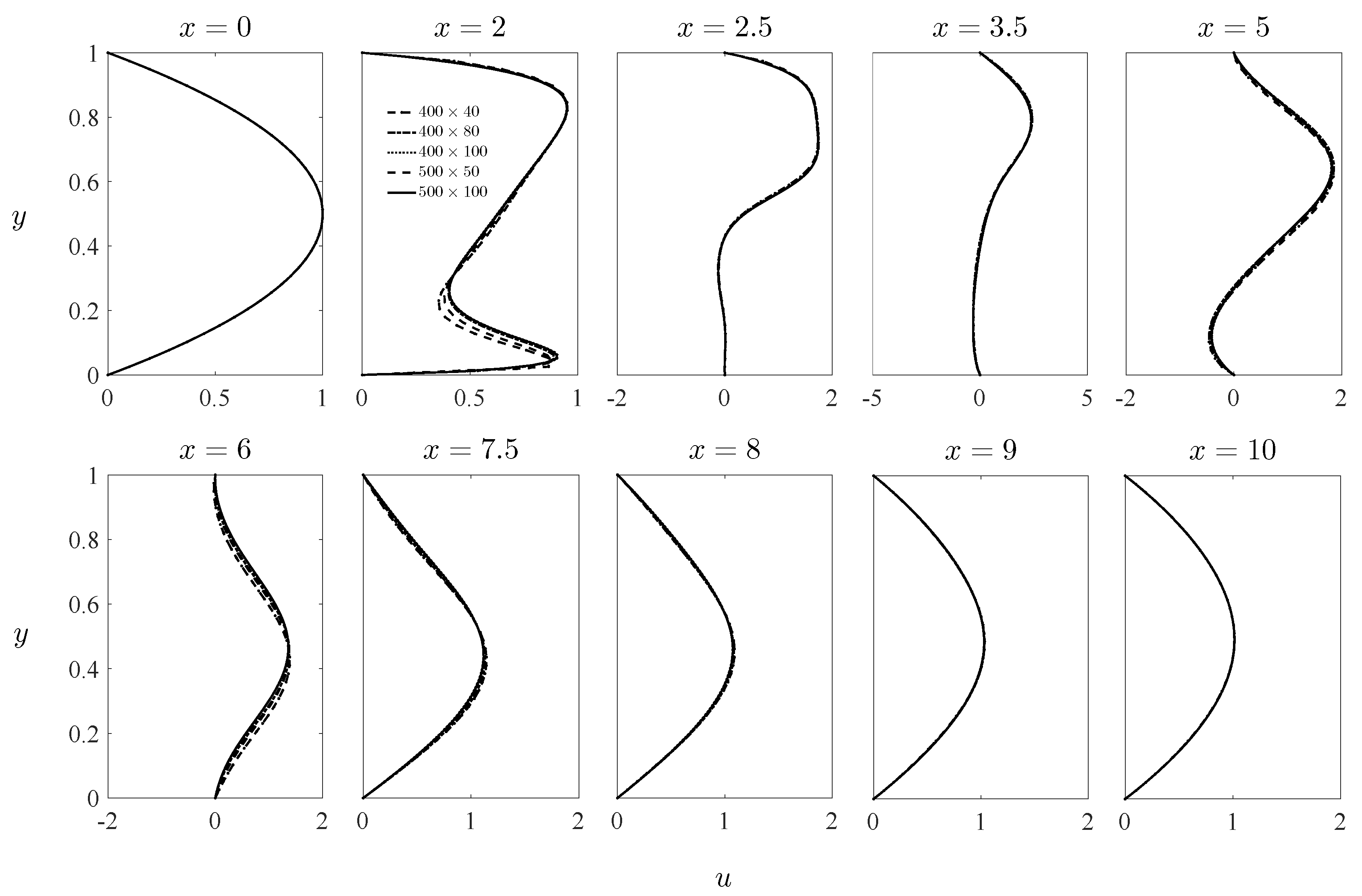
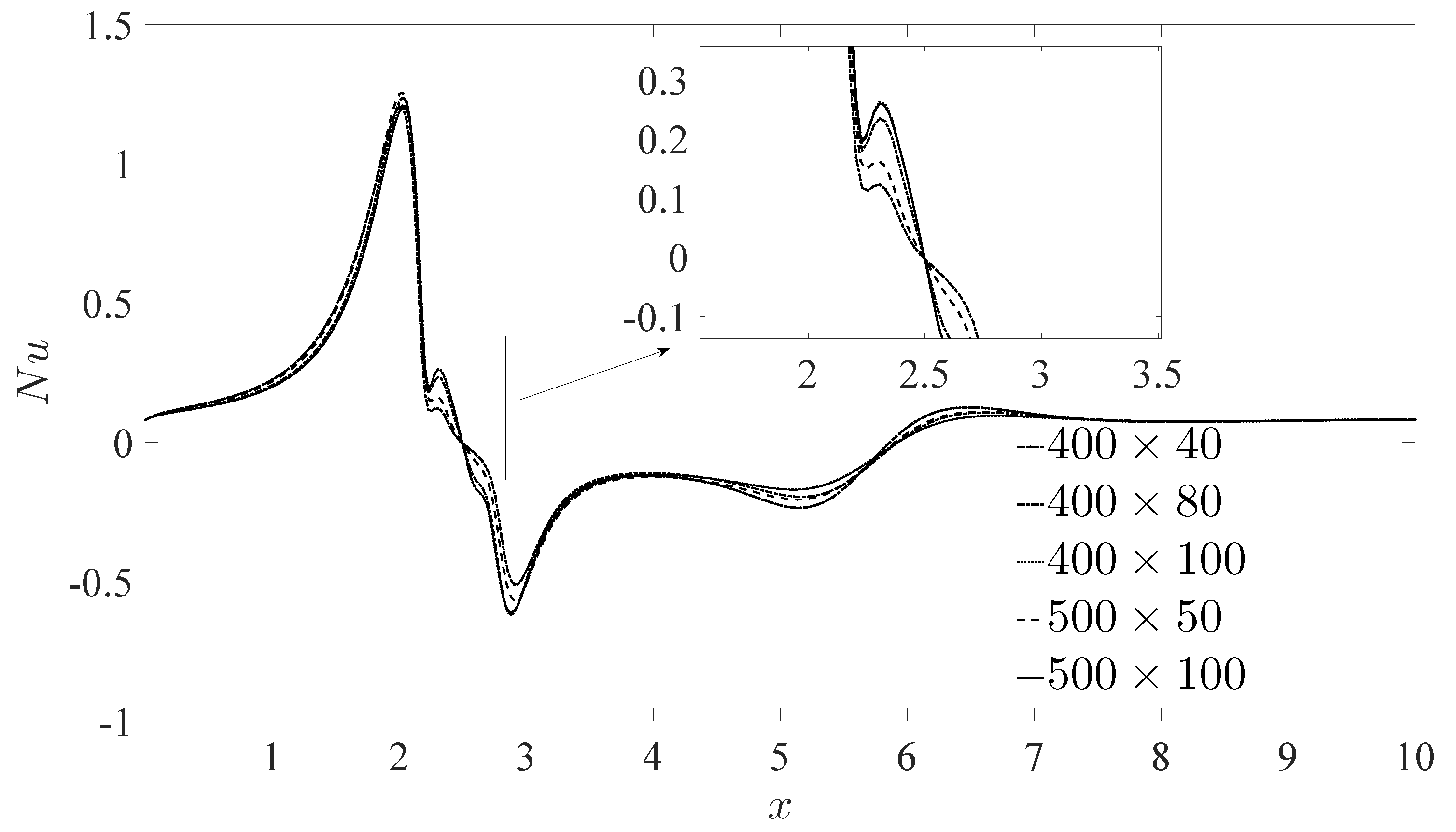
Numerical solution of the system of Equations (18)–(20) has been developed using Matlab^®. An extensive grid independence test is performed to check for the grid independent solution. The test is based on the u-velocity profile along the various x location of the channel, where the focus is emphasised near the location on the magnetic source. Five different size of grids configuration have been performed on the case flow problem $n=1$, $M{n}_F=1312$ and $N=0.056$. The magnetic source is located at $(a,b)=(2.5,-0.05)$. As shown in Figure 2, when the grid size is refined from $400\times 40$ to $500\times 100$, there is a significant change on velocity profile, particularly near the magnetic source and in the interval of the vortex size. The numerical simulation is sensitive on the vertical grid, while no significant change occurred when refining the horizontal grid. For the temperature profile, the local heat transfer on the lower wall of the channel has been used as a reference to test the grid independence. Only the lower wall is shown since most of the significant changes occurred near the magnetic source. The same grid independence test result is observed as seen in Figure 3, where the grids size have reached grid independence for temperature profile. These grids sizes have also been tested with smaller time step and no significant changes is accounted. It is observed that the grid size configuration of $400\times 80$ is sufficient to capture the velocity profile change near the magnetic location.

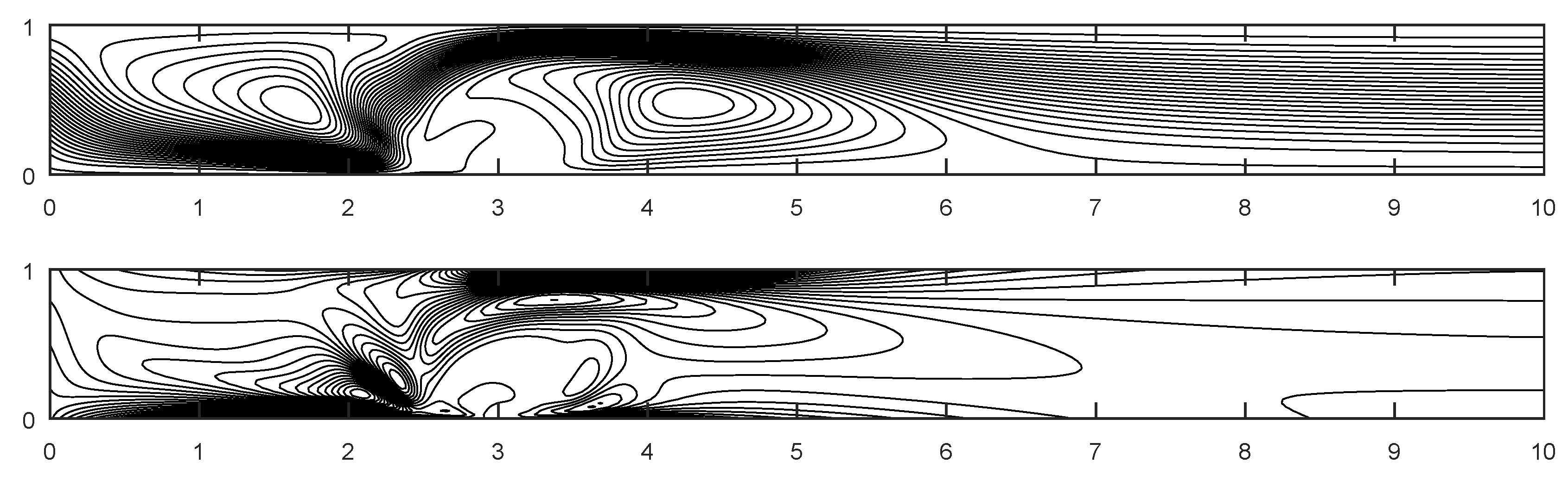
The performance and the validation of present numerical method, are done separately on the benchmark cases for non-Newtonian flow in lid driven cavity, and for the flow in a channel undergoing the localised magnetic field. The results validation regarding the flow in a channel under the action of localised magnetic field is performed as in [33]. From Figure 4, it can be seen that the present numerical method developed is in good agreement with the compared studies.

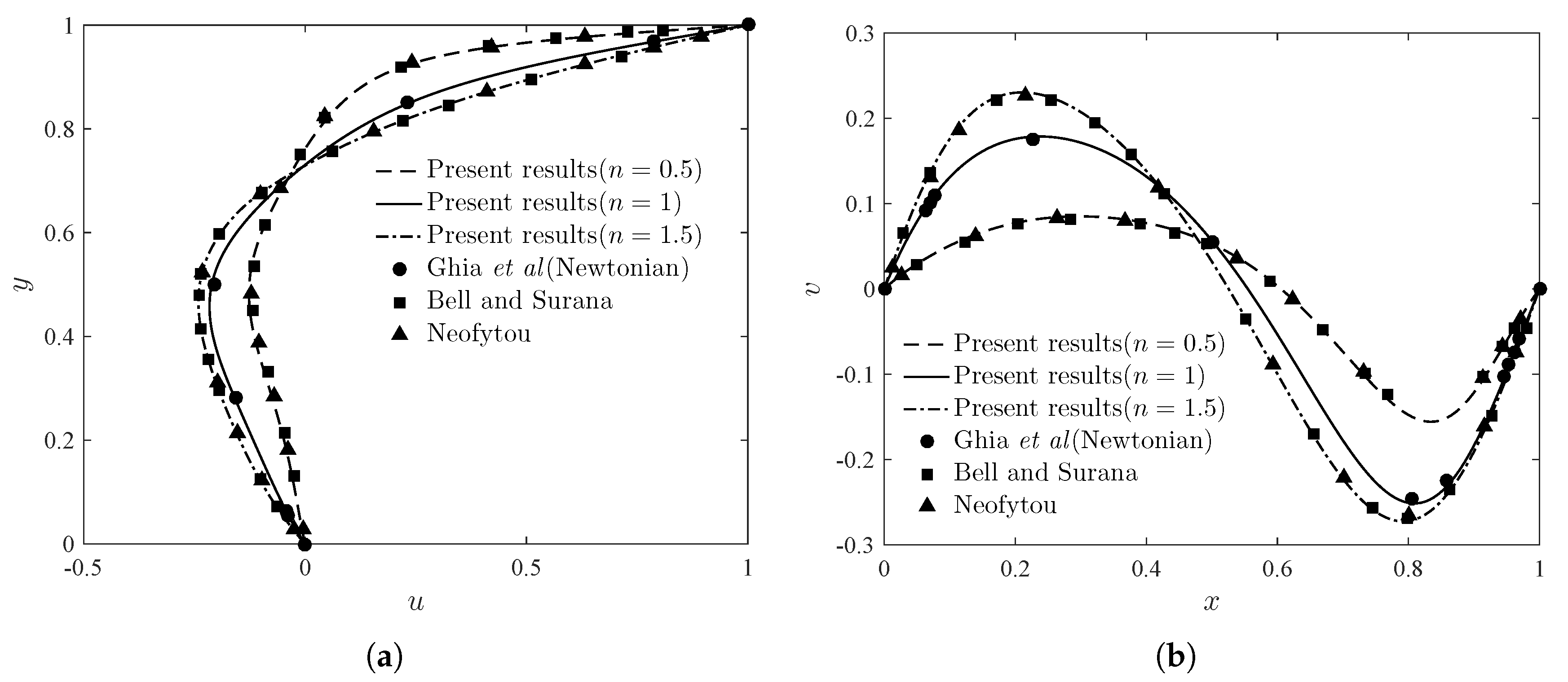
The second validation of the code is based on the non-Newtonian comparison. The computation involving non-Newtonian of power-law model in a lid driven cavity is validated with the works of Bell and Surana [60] and Neofytou [61]. In accordance with these works, simulations have been performed for $Re=100$ with different values of the power-law index. For Newtonian flow case, the comparison is made with the benchmark works of Ghia et al. [80]. The grid size used is $150\times 150,$ with the dimension of the wall is $1\times 1$ where the top wall is moving with velocity $u=1.$ Figure 5a shows the results for u-velocity along the vertical centreline and the Figure 5b v-velocity along the horizontal centreline. The non-Newtonian cases for $n=0.5$ and $n=1.5$ show very good agreement when compared with the results by Bell and Surana [60] and Neofytou [61]. For $n=1$, the result is in very good agreement with the result by Ghia et al. [80].

4. Results and Discussion

The time step is chosen to be $\Delta t={10}^{-4}$ for Newtonian and shear thickening cases while for shear thinning cases, the value of $\Delta t={10}^{-5}$ is required for the numerical method to converge. For shear thinning fluid the lowest number of power-law index in this work that converged is $n=0.6$ while the shear thickening cases were tested until $n=1.5$, although only the results for $n=0.6$, $n=1$ and $n=1.4$ are shown.

The flow is purely FHD by setting $N=0$, and will be purely MHD if $M{n}_F=0.$ When both $M{n}_F$ and N are zero, there is no magnetic source and the flow is purely hydrodynamics hence the flow in the channel has horizontal streamline corresponds to the parabolic profile for u-velocity. When the magnetic source is applied, a vortex arises near the area of the magnetic source. This phenomenon of how the flow is affected by the applied magnetic source with the variation of the power-law index is the main interest of this work. When the flow is tested on pure MHD, the effect of the magnetic field is not significant as the value of Stuart number N that is required to induced the vortex in the area of magnetic source has to be in the order of hundreds and the change is negligible even when N is increased into the order of thousands.

Figure 6 shows the streamlines contours for variations of power-law index $n=0.6,1.0$ and $n=1.4$, with variation of reference magnetic field ${\overline{B}}_0=1$ T, ${\overline{B}}_0=4$ T, and ${\overline{B}}_0=8$ T. The notable effect of applying magnetic field on the flow is the formation of arising vortex near the location of magnetic field. As discussed in previous literature, this vortex extension increases with the increment of magnetic field from 1 T to 8 T. Interesting results are observed when the power-law index is increased from $n=0.6$ to $1.4$, the disturbance in the flow field is also affected. For the case of shear thinning fluid $n=0.6$ it can be seen that the extension of the vortex is large and extended towards the downstream, compared to the case of when $n=1.0$ and $n=1.4$. Additionally when $n=1.4$, the vortex formation is smaller although its size increases when the Magnetic number is increased. The measured range of sizes of the vortex for each cases summarised in

Table 2. Range of vortex for different Magnetic numbers at various power-law index.

n	${\overline{\mathit{B}}}_0=1$ T	${\overline{\mathit{B}}}_0=4$ T	${\overline{\mathit{B}}}_0=8$ T
$n=0.6$	$2<x<5.66$	$2<x<7.61$	$2<x<8.42$
$n=1.0$	$2<x<4.69$	$2<x<5.59$	$2<x<5.94$
$n=1.4$	$2<x<4.04$	$2<x<4.61$	$2<x<4.87$

.

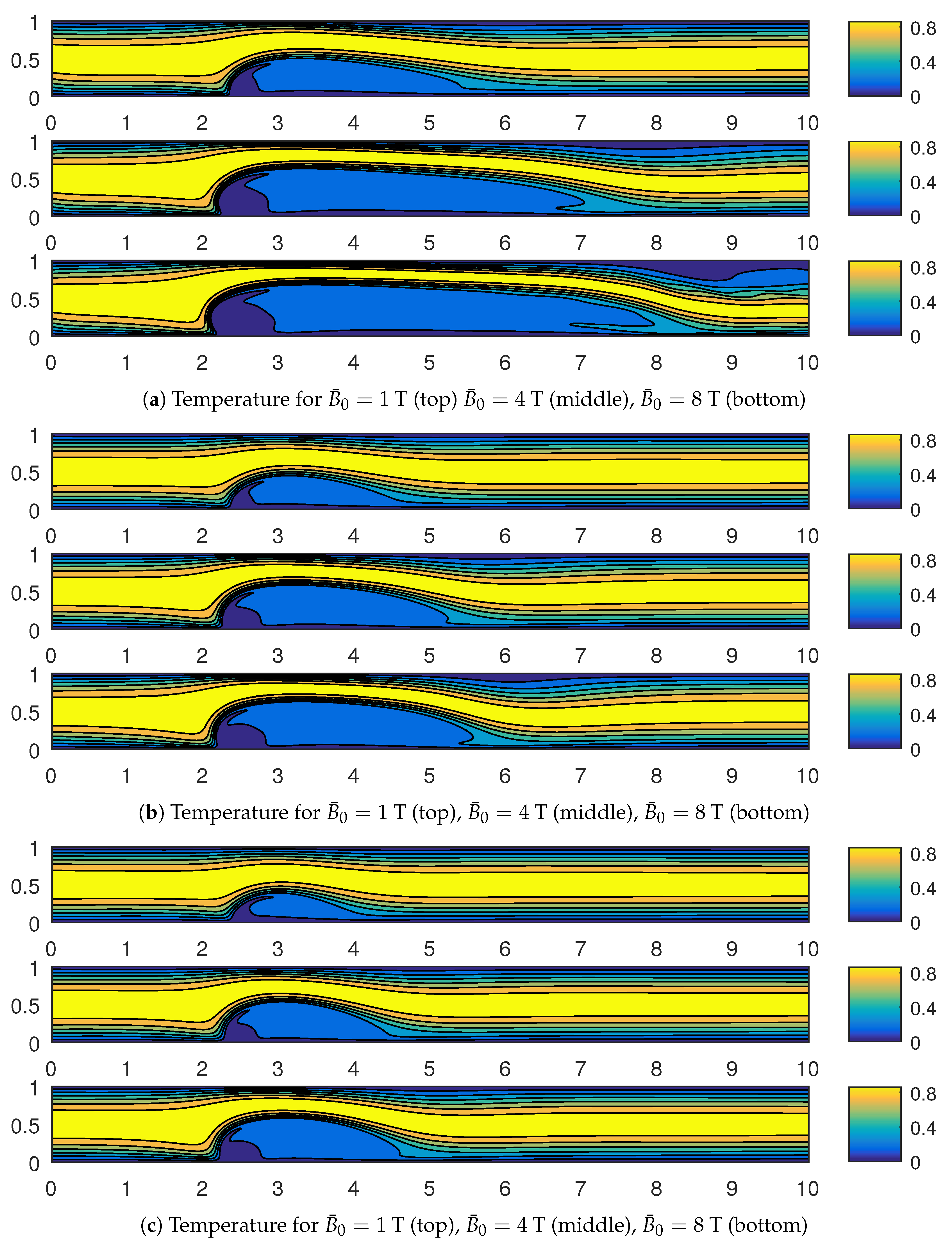
Figure 7 shows the corresponding temperature contours for variations of power-law with variation of reference magnetic corresponds to the case presented in Figure 6. It is shown that in the area of magnetic source, the maximum temperature is displaced towards the upper plate. The effect is more pronounced when the Magnetic number is increased, regardless the power-law index. The region of the lower vortex is shown to be kept cooler and this region is extended towards the downstream when the Magnetic number is increased for all the cases of different power-law index.

From the previous discussion, it can be seen that the influence of increasing power-law index number n has the opposite effect to the increasing Magnetic numbers on the flow field.

Table 3. Minimum u-velocity for different Magnetic numbers at various power-law index.

	${\overline{\mathit{B}}}_0=1$ T	${\overline{\mathit{B}}}_0=4$ T	${\overline{\mathit{B}}}_0=8$ T
$n=0.6$	$u_{min}=-0.1792$	$u_{min}=-0.2831$	$u_{min}=-0.4106$
$n=1.0$	$u_{min}=-0.2258$	$u_{min}=-0.3783$	$u_{min}=-0.4848$
$n=1.4$	$u_{min}=-0.2357$	$u_{min}=-0.4068$	$u_{min}=-0.5093$

shows the minimum velocity for different Magnetic numbers at various power-law index. The negative symbol indicates the direction of the velocity and the reverse flow of the vortex region near the magnetic source. From Magnetic number 1 T to 8 T the minimum u-velocity is increased for every n. Overall, the shear thickening flow has the highest velocity followed by Newtonian and shear thinning flow.

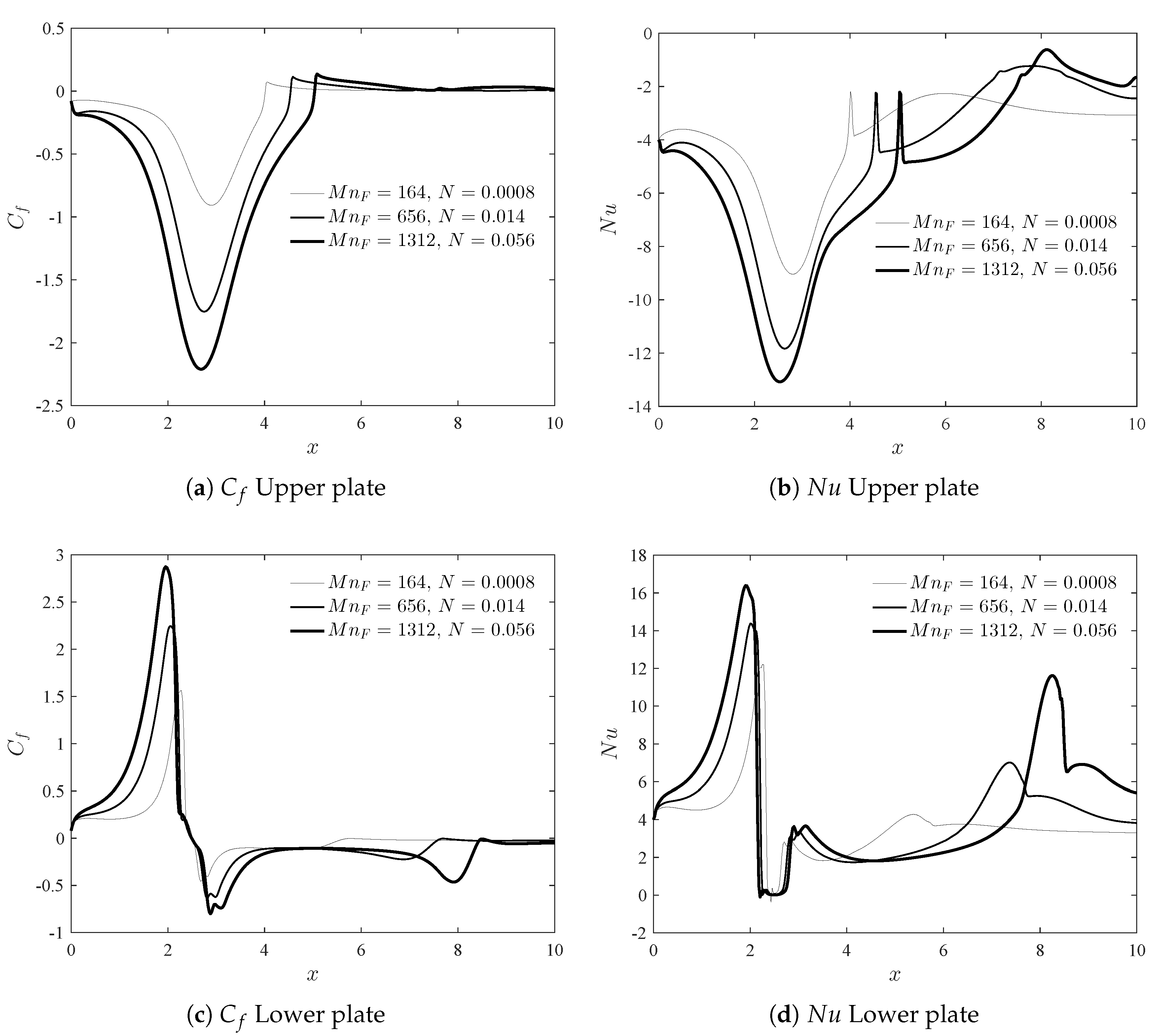
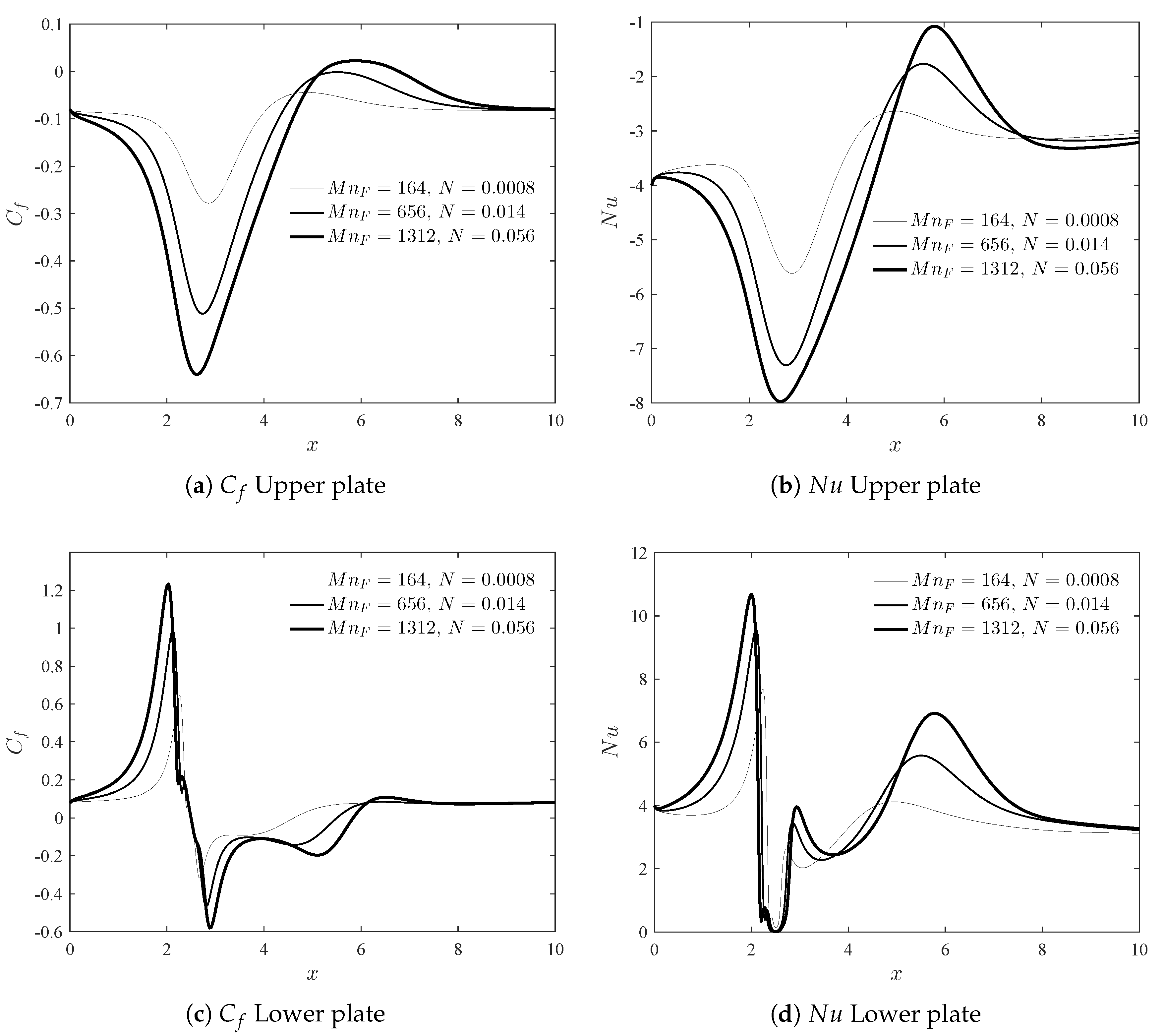
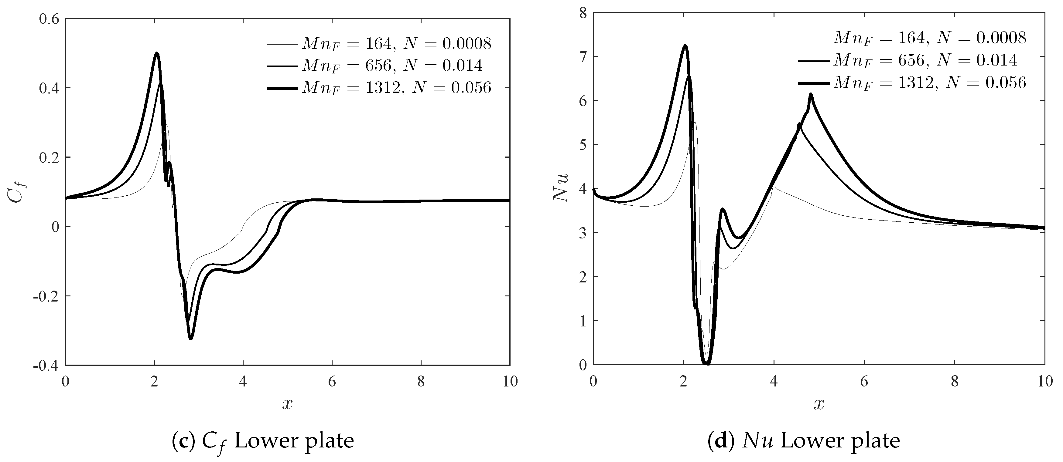
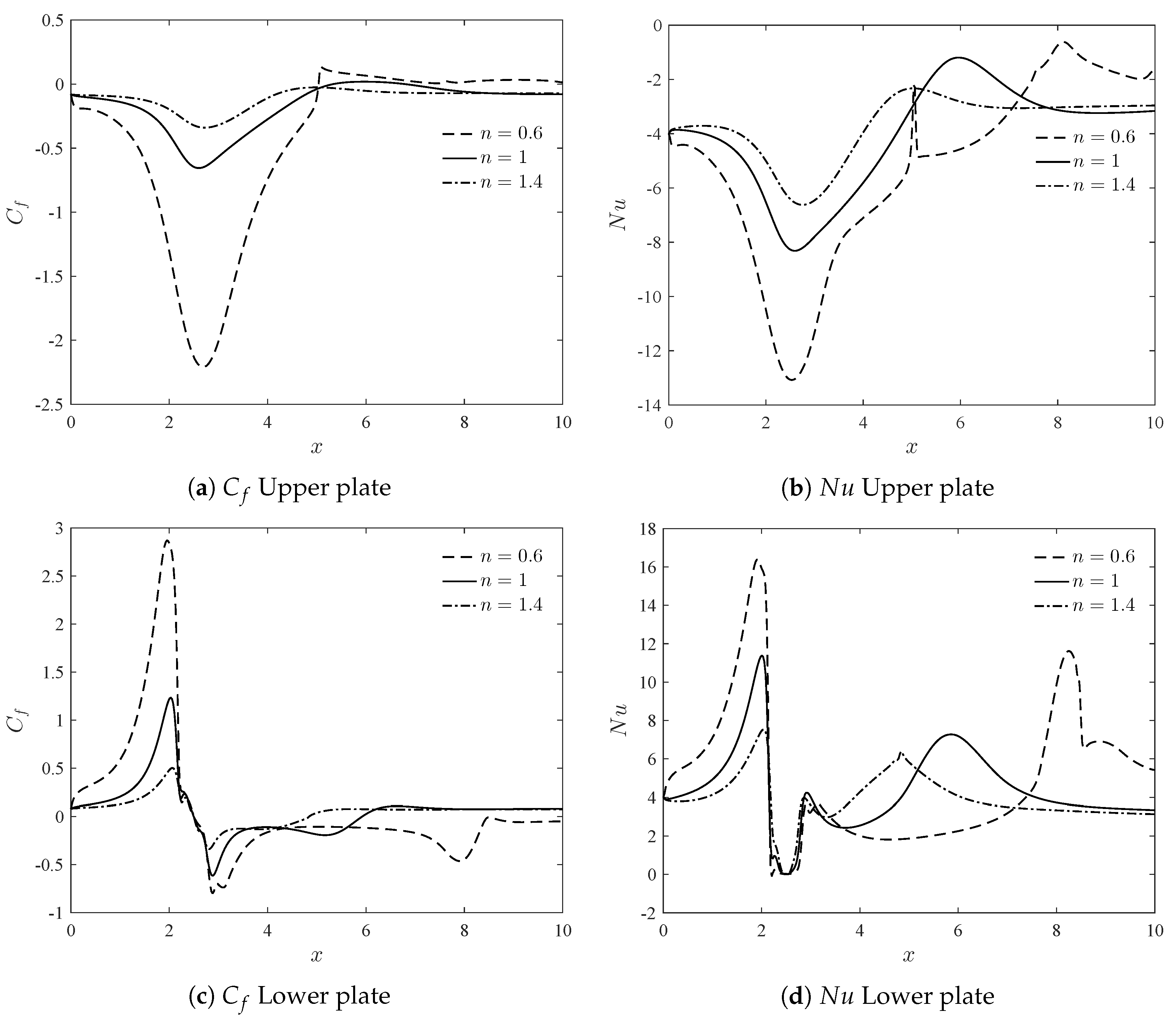
The variation of wall shear stress and heat transfer parameters of various Magnetic numbers for $n=0.6$, $n=1.0$ and $n=1.4$ are shown in Figure 8, Figure 9 and Figure 10 respectively. The wall shear stress are shown to have more influence on the lower plate, particularly at the location of the magnetic source. The variation of this parameter is qualitatively the same as magnetic field are varied from 1 T to 8 T, where the higher magnetic field results in greater variation of the wall shear stress irrespective the value of n. The variation of wall shear for the upper wall (Figure 8a, Figure 9a and Figure 10a) for all cases changes smoothly from increasing to decreasing near the area of the magnetic source, and its sign does not change. For the upper wall, the lower values of this parameter indicates the higher rates of skin friction. For the case of the lower wall (Figure 8c, Figure 9c and Figure 10c), the rapid changes of this parameter is largest for the case of shear thinning flow, followed by Newtonian and shear thickening flow as shown by the difference of the extrema values. For the lower wall, the negative values of the wall shear stress refers to inversion of the flow, and when wall shear stress reach its original value at $x=0$, it refers to fully developed flow. This indicator is used to verify that all the flow cases managed to revert back to fully developed flow when it reaches downstream.

The heat transfer parameters for the upper wall (Figure 8b, Figure 9b and Figure 10b) and lower wall (Figure 8d, Figure 9d and Figure 10d) similarly shows the same qualitative variation when magnetic fields are varied from 1 T to 8 T, for each case flow. On the lower wall, it is shown that the rate of heat transfer increases when Magnetic number increases, regardless the power-law index. For the case of $n=0.6$, the overall heat transfer to lower wall is greater than the case of $n=1.0$ and $n=1.4$. The heat transfer coefficient is relatively high near the location of magnetic source, and another second region reaching the downstream due to the disturbance of the temperature field is extended far downstream. These second location of high heat transfer coefficient are observed at region $5.5<x<8.5$, $4.5<x<6$ and $4<x<5$ for $n=0.6$, $n=1.0$ and $n=1.4$ respectively. On the upper wall, the lower values of this coefficient refers to higher rates of heat transfer to the wall and it exhibits a similarity with the case of the lower wall.

Another quantitative comparison can be made from Figure 11, for different power-law index n and magnetic field at 8 T, where it shows that the wall shear stress and heat transfer parameters are highest for the case of shear thinning flow, followed by Newtonian and shear thickening.

5. Conclusions

In this paper, the effect of magnetic field on non-Newtonian biomagnetic power-law flow in a channel has been studied numerically by Constrained Interpolated Profile Finite Difference Method (CIP-FDM). This study has been conducted for the parameters ${\overline{B}}_0=1$ T, ${\overline{B}}_0=4$ T and ${\overline{B}}_0=8$ T for power-law index $n=0.6$ (shear thinning), $n=1$ (Newtonian) and $n=1.4$ (shear thickening). The investigation is performed based on the study of the streamline, temperature, vorticity contours, wall shear stress and heat transfer parameters. A good agreement validated with previous numerical investigation demonstrates that the CIP-FDM is an appropriate method for the power-law flow in a channel under an applied magnetic field. The enhancement of Magnetic number increases the length of vortex formation regardless the power-law index. The consideration of power-law index, causes the size of vortex formation to expand in shear thinning flow, and shrink in shear thickening flow. The amplification of Magnetic number increases both the wall shear stress and the heat transfer parameters dominantly near the location of magnetic source. The opposite effect is observed when the power-law is included as the wall shear stress and heat transfer parameters are decreased. The work reported here shows the severe drawbacks associated with RF radiation to blood vessel locally on the displacement of the high temperature and the blockage due to back flow. For future research, it is recommended to perform an analysis on fluid structure interaction by calculating the elastic deformation of the vessel.

References

- Jain, V.; Abdulmalik, O.; Propert, K.J.; Wehrli, F.W. Investigating the magnetic susceptibility properties of fresh human blood for noninvasive oxygen saturation quantification. Magn. Reson. Med. 2012, 68, 863–867. [Google Scholar] [CrossRef] [Green Version]
- Tzirtzilakis, E.; Loukopoulos, V. Biofluid flow in a channel under the action of a uniform localized magnetic field. Comput. Mech. 2005, 36, 360–374. [Google Scholar] [CrossRef]
- Haik, Y.; Chen, C.J.; Chatterjee, J. Numerical simulation of biomagnetic fluid in a channel with thrombus. J. Vis. 2002, 5, 187–195. [Google Scholar] [CrossRef]
- Neuringer, J.L.; Rosensweig, R.E. Ferrohydrodynamics. Phys. Fluids 1964, 7, 1927–1937. [Google Scholar] [CrossRef]
- Voltairas, P.; Fotiadis, D.; Michalis, L. Hydrodynamics of magnetic drug targeting. J. Biomech. 2002, 35, 813–821. [Google Scholar] [CrossRef]
- Ruuge, E.; Rusetski, A. Magnetic fluids as drug carriers: Targeted transport of drugs by a magnetic field. J. Magn. Magn. Mater. 1993, 122, 335–339. [Google Scholar] [CrossRef]
- Fiorentini, G.; Szasz, A. Hyperthermia today: Electric energy, a new opportunity in cancer treatment. J. Cancer Res. Ther. 2006, 2, 41. [Google Scholar] [CrossRef]
- Plavins, J.; Lauva, M. Study of colloidal magnetite-binding erythrocytes: Prospects for cell separation. J. Magn. Magn. Mater. 1993, 122, 349–353. [Google Scholar] [CrossRef]
- Raj, K.; Moskowitz, B.; Tsuda, S. New commercial trends of nanostructured ferrofluids. Indian J. Eng. Mater. Sci. 2004, 11, 241–252. [Google Scholar]
- Scherer, C.; Figueiredo Neto, A.M. Ferrofluids: Properties and applications. Braz. J. Phys. 2005, 35, 718–727. [Google Scholar] [CrossRef]
- Odenbach, S. Colloidal Magnetic Fluids: Basics, Development and Application of Ferrofluids; Springer: Berlin/Heidelberg, Germany, 2009; Volume 763. [Google Scholar] [CrossRef] [Green Version]
- Kıvrak, E.G.; Yurt, K.K.; Kaplan, A.A.; Alkan, I.; Altun, G. Effects of electromagnetic fields exposure on the antioxidant defense system. J. Microsc. Ultrastruct. 2017, 5, 167–176. [Google Scholar] [CrossRef]
- Fragopoulou, A.F.; Koussoulakos, S.L.; Margaritis, L.H. Cranial and postcranial skeletal variations induced in mouse embryos by mobile phone radiation. Pathophysiology 2010, 17, 169–177. [Google Scholar] [CrossRef]
- Van den Brink, J.S. Thermal Effects Associated with RF Exposures in Diagnostic MRI: Overview of Existing and Emerging Concepts of Protection. Concepts Magn. Reson. Part B 2019, 2019, 9618680. [Google Scholar] [CrossRef] [Green Version]
- Zhang, X.; Yarema, K.; Xu, A. Biological Effects of Static Magnetic Fields; Springer: Singapore, 2017. [Google Scholar]
- Duan, G.; Zhao, X.; Anderson, S.W.; Zhang, X. Boosting magnetic resonance imaging signal-to-noise ratio using magnetic metamaterials. Commun. Phys. 2019, 2, 1–8. [Google Scholar] [CrossRef]
- Nowogrodzki, A. The world’s strongest MRI machines are pushing human imaging to new limits. Nature 2018, 563, 24–27. [Google Scholar] [CrossRef]
- Ichioka, S.; Minegishi, M.; Iwasaka, M.; Shibata, M.; Nakatsuka, T.; Harii, K.; Kamiya, A.; Ueno, S. High-intensity static magnetic fields modulate skin microcirculation and temperature in vivo. Bioelectromagn. J. Bioelectromagn. Soc. 2000, 21, 183–188. [Google Scholar] [CrossRef]
- Haik, Y.; Pai, V.; Chen, C. Biomagnetic fluid dynamics. In Fluid Dyn. Interfaces; Shyy, W., Narayanan, R., Eds.; Cambridge University Press: Cambridge, UK, 1999; pp. 439–452. [Google Scholar]
- Motta, M.; Haik, Y.; Gandhari, A.; Chen, C.J. High magnetic field effects on human deoxygenated hemoglobin light absorption. Bioelectrochem. Bioenergy 1998, 47, 297–300. [Google Scholar] [CrossRef]
- Higashi, T.; Yamagishi, A.; Takeuchi, T.; Kawaguchi, N.; Sagawa, S.; Onishi, S.; Date, M. Orientation of erythrocytes in a strong static magnetic field. Blood 1993, 82, 1328–1334. [Google Scholar] [CrossRef] [Green Version]
- Khashan, S.A.; Haik, Y. Numerical simulation of biomagnetic fluid downstream an eccentric stenotic orifice. Phys. Fluids 2006, 18, 113601. [Google Scholar] [CrossRef]
- Loukopoulos, V.; Tzirtzilakis, E. Biomagnetic channel flow in spatially varying magnetic field. Int. J. Eng. Sci. 2004, 42, 571–590. [Google Scholar] [CrossRef]
- Tzirtzilakis, E. A mathematical model for blood flow in magnetic field. Phys. Fluids 2005, 17, 077103. [Google Scholar] [CrossRef]
- Rosensweig, R.E. Ferrohydrodynamics, Reprinted ed.; Dover Publications: Mineola, NY, USA, 2013. [Google Scholar]
- Sahoo, B.C.; Vajjha, R.S.; Ganguli, R.; Chukwu, G.A.; Das, D.K. Determination of rheological behavior of aluminum oxide nanofluid and development of new viscosity correlations. Pet. Sci. Technol. 2009, 27, 1757–1770. [Google Scholar] [CrossRef]
- Zhou, S.Q.; Ni, R.; Funfschilling, D. Effects of shear rate and temperature on viscosity of alumina polyalphaolefins nanofluids. J. Appl. Phys. 2010, 107, 054317. [Google Scholar] [CrossRef]
- Odenbach, S.; Thurm, S. Magnetoviscous effects in ferrofluids. In Ferrofluids; Springer: Berlin/Heidelberg, Germany, 2002; pp. 185–201. [Google Scholar] [CrossRef]
- Odenbach, S. Ferrofluids: Magnetically Controllable Fluids and Their Applications; Springer: Berlin/Heidelberg, Germany, 2008; Volume 594. [Google Scholar] [CrossRef]
- Goharkhah, M.; Ashjaee, M. Effect of an alternating nonuniform magnetic field on ferrofluid flow and heat transfer in a channel. J. Magn. Magn. Mater. 2014, 362, 80–89. [Google Scholar] [CrossRef]
- Tzirtzilakis, E.; Xenos, M.; Loukopoulos, V.; Kafoussias, N. Turbulent biomagnetic fluid flow in a rectangular channel under the action of a localized magnetic field. Int. J. Eng. Sci. 2006, 44, 1205–1224. [Google Scholar] [CrossRef]
- Siddiqa, S.; Naqvi, S.; Begum, N.; Awan, S.; Hossain, M. Thermal radiation therapy of biomagnetic fluid flow in the presence of localized magnetic field. Int. J. Therm. Sci. 2018, 132, 457–465. [Google Scholar] [CrossRef]
- Tzirtzilakis, E. A simple numerical methodology for BFD problems using stream function vorticity formulation. Commun. Numer. Methods Eng. 2008, 24, 683–700. [Google Scholar] [CrossRef]
- Xenos, M.; Tzirtzilakis, E. MHD effects on blood flow in a stenosis. Adv. Dyn. Syst. Appl. 2013, 8, 427–437. [Google Scholar]
- Türk, Ö.; Tezer-Sezgin, M.; Bozkaya, C. Finite element study of biomagnetic fluid flow in a symmetrically stenosed channel. J. Comput. Appl. Math. 2014, 259, 760–770. [Google Scholar] [CrossRef]
- Türk, Ö.; Bozkaya, C.; Tezer-Sezgin, M. A FEM approach to biomagnetic fluid flow in multiple stenosed channels. Comput. Fluids 2014, 97, 40–51. [Google Scholar] [CrossRef]
- Tzirtzilakis, E. Biomagnetic fluid flow in an aneurysm using ferrohydrodynamics principles. Phys. Fluids 2015, 27, 061902. [Google Scholar] [CrossRef]
- Sharifi, A.; Motlagh, S.Y.; Badfar, H. Numerical investigation of magnetic drug targeting using magnetic nanoparticles to the Aneurysmal Vessel. J. Magn. Magn. Mater. 2019, 474, 236–245. [Google Scholar] [CrossRef]
- Tzirakis, K.; Papaharilaou, Y.; Giordano, D.; Ekaterinaris, J. Numerical investigation of biomagnetic fluids in circular ducts. Int. J. Numer. Methods Biomed. Eng. 2014, 30, 297–317. [Google Scholar] [CrossRef] [PubMed]
- Tzirtzilakis, E.; Xenos, M. Biomagnetic fluid flow in a driven cavity. Meccanica 2013, 48, 187–200. [Google Scholar] [CrossRef]
- Marioni, L.; Bay, F.; Hachem, E. Numerical stability analysis and flow simulation of lid-driven cavity subjected to high magnetic field. Phys. Fluids 2016, 28, 057102. [Google Scholar] [CrossRef]
- Bozkaya, N.; Tezer-Sezgin, M. The DRBEM solution of incompressible MHD flow equations. Int. J. Numer. Methods Fluids 2011, 67, 1264–1282. [Google Scholar] [CrossRef]
- Senel, P.; Tezer-Sezgin, M. DRBEM solutions of Stokes and Navier–Stokes equations in cavities under point source magnetic field. Eng. Anal. Bound. Elem. 2016, 64, 158–175. [Google Scholar] [CrossRef]
- Kefayati, G.R. Simulation of magnetic field effect on non-Newtonian blood flow between two-square concentric duct annuli using FDLBM. J. Taiwan Inst. Chem. Eng. 2014, 45, 1184–1196. [Google Scholar] [CrossRef]
- Kefayati, G.R. Simulation of heat transfer and entropy generation of MHD natural convection of non-Newtonian nanofluid in an enclosure. Int. J. Heat Mass Transf. 2016, 92, 1066–1089. [Google Scholar] [CrossRef]
- Adıgüzel, Ö.B.; Atalık, K. Magnetic field effects on Newtonian and non-Newtonian ferrofluid flow past a circular cylinder. Appl. Math. Model. 2017, 42, 161–174. [Google Scholar] [CrossRef]
- Jahanbakhshi, A.; Nadooshan, A.A.; Bayareh, M. Magnetic field effects on natural convection flow of a non-Newtonian fluid in an L-shaped enclosure. J. Therm. Anal. Calorim. 2018, 133, 1407–1416. [Google Scholar] [CrossRef]
- Ikbal, M.A.; Chakravarty, S.; Wong, K.K.; Mazumdar, J.; Mandal, P.K. Unsteady response of non-Newtonian blood flow through a stenosed artery in magnetic field. J. Comput. Appl. Math. 2009, 230, 243–259. [Google Scholar] [CrossRef]
- Sankar, D.; Lee, U. FDM analysis for MHD flow of a non-Newtonian fluid for blood flow in stenosed arteries. J. Mech. Sci. Technol. 2011, 25, 2573. [Google Scholar] [CrossRef]
- Haynes, R.H.; Burton, A.C. Role of the non-Newtonian behavior of blood in hemodynamics. Am. J. Physiol.-Leg. Content 1959, 197, 943–950. [Google Scholar] [CrossRef] [PubMed] [Green Version]
- Chien, S.; Usami, S.; Taylor, H.M.; Lundberg, J.L.; Gregersen, M.I. Effects of hematocrit and plasma proteins on human blood rheology at low shear rates. J. Appl. Physiol. 1966, 21, 81–87. [Google Scholar] [CrossRef]
- Shukla, J.; Parihar, R.; Rao, B. Effects of stenosis on non-Newtonian flow of the blood in an artery. Bull. Math. Biol. 1980, 42, 283–294. [Google Scholar] [CrossRef]
- Pedley, T.J. The Fluid Mechanics of Large Blood Vessels; Cambridge University Press: Cambridge, UK, 1980. [Google Scholar] [CrossRef]
- Berger, S.; Jou, L.D. Flows in stenotic vessels. Annu. Rev. Fluid Mech. 2000, 32, 347–382. [Google Scholar] [CrossRef]
- Easthope, P.; Brooks, D. A comparison of rheological constitutive functions for whole human blood. Biorheology 1980, 17, 235–247. [Google Scholar]
- Walburn, F.J.; Schneck, D.J. A constitutive equation for whole human blood. Biorheology 1976, 13, 201–210. [Google Scholar] [CrossRef]
- Cho, Y.I.; Kensey, K.R. Effects of the non-Newtonian viscosity of blood on flows in a diseased arterial vessel. Part 1: Steady flows. Biorheology 1991, 28, 241–262. [Google Scholar] [CrossRef]
- Quemada, D. A non-linear Maxwell model of biofluids: Application to normal blood. Biorheology 1993, 30, 253–265. [Google Scholar] [CrossRef] [PubMed]
- Boyd, J.; Buick, J.M.; Green, S. Analysis of the Casson and Carreau-Yasuda non-Newtonian blood models in steady and oscillatory flows using the lattice-Boltzmann method. Phys. Fluids 2007, 19, 093103. [Google Scholar] [CrossRef] [Green Version]
- Bell, B.C.; Surana, K.S. P-version least squares finite element formulation for two-dimensional, incompressible, non-Newtonian isothermal and non-isothermal fluid flow. Int. J. Numer. Methods Fluids 1994, 18, 127–162. [Google Scholar] [CrossRef]
- Neofytou, P. A 3rd order upwind finite volume method for generalised Newtonian fluid flows. Adv. Eng. Softw. 2005, 36, 664–680. [Google Scholar] [CrossRef]
- Misra, J.; Shit, G.; Rath, H.J. Flow and heat transfer of a MHD viscoelastic fluid in a channel with stretching walls: Some applications to haemodynamics. Comput. Fluids 2008, 37, 1–11. [Google Scholar] [CrossRef] [Green Version]
- Liu, I.C. Flow and heat transfer of an electrically conducting fluid of second grade in a porous medium over a stretching sheet subject to a transverse magnetic field. Int. J. Non-Linear Mech. 2005, 40, 465–474. [Google Scholar] [CrossRef]
- Rosti, M.E.; Picano, F.; Brandt, L. Numerical approaches to complex fluids. In Flowing Matter; Springer: Cham, Switzerland, 2019; pp. 1–34. [Google Scholar] [CrossRef] [Green Version]
- Tzirtzilakis, E. Biomagnetic fluid flow in a channel with stenosis. Phys. D Nonlinear Phenom. 2008, 237, 66–81. [Google Scholar] [CrossRef]
- Sheikholeslami, M.; Bandpy, M.G.; Ellahi, R.; Zeeshan, A. Simulation of MHD CuO–water nanofluid flow and convective heat transfer considering Lorentz forces. J. Magn. Magn. Mater. 2014, 369, 69–80. [Google Scholar] [CrossRef]
- Sheikholeslami, M.; Ellahi, R. Three dimensional mesoscopic simulation of magnetic field effect on natural convection of nanofluid. Int. J. Heat Mass Transf. 2015, 89, 799–808. [Google Scholar] [CrossRef]
- Sheikholeslami, M.; Ganji, D.D. Ferrohydrodynamic and magnetohydrodynamic effects on ferrofluid flow and convective heat transfer. Energy 2014, 75, 400–410. [Google Scholar] [CrossRef]
- Sheikholeslami, M.; Rashidi, M.; Ganji, D. Effect of non-uniform magnetic field on forced convection heat transfer of Fe3O4–water nanofluid. Comput. Methods Appl. Mech. Eng. 2015, 294, 299–312. [Google Scholar] [CrossRef]
- Sheikholeslami, M.; Vajravelu, K.; Rashidi, M.M. Forced convection heat transfer in a semi annulus under the influence of a variable magnetic field. Int. J. Heat Mass Transf. 2016, 92, 339–348. [Google Scholar] [CrossRef]
- Rashidi, S.; Esfahani, J.A.; Maskaniyan, M. Applications of magnetohydrodynamics in biological systems-a review on the numerical studies. J. Magn. Magn. Mater. 2017, 439, 358–372. [Google Scholar] [CrossRef]
- Yabe, T.; Takizawa, K.; Chino, M.; Imai, M.; Chu, C. Challenge of CIP as a universal solver for solid, liquid and gas. Int. J. Numer. Methods Fluids 2005, 47, 655–676. [Google Scholar] [CrossRef]
- Takewaki, H.; Nishiguchi, A.; Yabe, T. Cubic interpolated pseudo-particle method (CIP) for solving hyperbolic-type equations. J. Comput. Phys. 1985, 61, 261–268. [Google Scholar] [CrossRef]
- Yabe, T.; Aoki, T. A universal solver for hyperbolic equations by cubic-polynomial interpolation I. One-dimensional solver. Comput. Phys. Commun. 1991, 66, 219–232. [Google Scholar] [CrossRef]
- Shi, Y.F.; Xu, B.; Guo, Y. Numerical solution of Korteweg-de Vries-Burgers equation by the compact-type CIP method. Adv. Differ. Equ. 2015, 2015, 353. [Google Scholar] [CrossRef] [Green Version]
- Yabe, T.; Wang, P.Y. Unified numerical procedure for compressible and incompressible fluid. J. Phys. Soc. Jpn. 1991, 60, 2105–2108. [Google Scholar] [CrossRef]
- Kishev, Z.R.; Hu, C.; Kashiwagi, M. Numerical simulation of violent sloshing by a CIP-based method. J. Mar. Sci. Technol. 2006, 11, 111–122. [Google Scholar] [CrossRef]
- Mussa, M.; Abdullah, S.; Azwadi, C.N.; Muhamad, N. Simulation of natural convection heat transfer in an enclosure by the lattice-Boltzmann method. Comput. Fluids 2011, 44, 162–168. [Google Scholar] [CrossRef]
- Yabe, T.; Aoki, T. A universal solver for hyperbolic-equation by cubic-polynomial interpolation. II. Two-and three dimensional solvers. Comput. Phys. Commun. 1991, 66, 233–242. [Google Scholar] [CrossRef]
- Ghia, U.; Ghia, K.N.; Shin, C. High-Re solutions for incompressible flow using the Navier-Stokes equations and a multigrid method. J. Comput. Phys. 1982, 48, 387–411. [Google Scholar] [CrossRef]
Figure 1.
Flow domain and contours of magnetic field strength H.
Figure 2.
Grid independence test for u-velocity profile at different locations x of the channel.
Figure 3.
Grid independence test of local heat transfer parameter on the channel’s lower wall.
Figure 4.
Stream function and vorticity contour for , = 131,250 obtained by using present method and comparable with [33].
Figure 5.
Comparison between present results and the results by Bell and Surana [60], Neofytou [61] for non-Newtonian power-law at various values of power-law index n, and Newtonian fluid flow by Ghia et al. [80]. (a) u-velocity profiles along the vertical centreline of the cavity. (b) v-velocity profiles along the horizontal centreline of the cavity for Re = 100.
Figure 6.
Streamline plot for power-law index: (a) n = 0.6 (shear thinning). (b) n = 1.0 (Newtonian). (c) n = 1.4 (shear thickening).
Figure 7.
Temperature plot for power-law index: (a) n = 0.6 (shear thinning). (b) n = 1.0 (Newtonian). (c) n = 1.4 (shear thickening).
Figure 8.
Variations of wall shear stress and heat transfer parameter for n = 0.6 with different intensity of magnetic field number.
Figure 9.
Variations of wall shear stress and heat transfer parameter for n = 1 with different intensity of magnetic field.
Figure 10.
Variations of wall shear stress and heat transfer parameter for with different intensity of magnetic field.
Figure 11.
Figure 11. Variations of wall shear stress parameter Cf and heat transfer parameter Nu for MnF = 1312, N = 0.056 for different power-law index n.