Modeling, Analysis and Experimental Validation of the Fuel Cell Association with DC-DC Power Converters with Robust and Anti-Windup PID Controller Design

Abstract

Based on full and rigorous study, this paper addresses the issue of ensuring a feasible association in practice between a Proton Exchange Membrane Fuel Cell (PEMFC) and DC-DC power converters including a buck and boost converter. This association is mathematically modeled, analyzed, and controlled by an optimal PID controller. Using absolute stability tools with a rigorous analytical approach that takes into consideration windup effects, in addition to the nonlinear behavior of the Proton Exchange Membrane Fuel Cell, sufficient conditions are provided to ensure that the closed-loop system is L₂-stable. These conditions allow the optimal PID controller parameters to be chosen and ensure the closed-loop system stability, by tracking reference outputs, and an optimal performance against perturbations. Formal analysis, numerical simulations, and experimental validation were carried out to verify that the PID controller designed with an anti-windup action is robust and meets all of the pre-defined objectives. Moreover, this study demonstrates that the association between the PEMFC and the DC-DC converters is achieved if only certain conditions are met.

1. Introduction

Currently, electric vehicles based on lithium-ion batteries dominate the market. However, the short longevity of lithium-ion batteries compared to their high cost is a disadvantage [1]. By comparison, fuel cells offer high energy density and super capacitors offer high power density with a very long service life (1 million recharge cycles) [2]. This complementarily is of interest to automobile manufacturers who are increasingly investigating the development of hybrid fuel cell vehicles [3,4].

Fuel cells are used as a source of electrical energy in many applications. They are proposed, among other things, as energy sources in electric motor vehicles (cars, buses, electrically propelled boats, etc.) to replace internal combustion engines. This would reduce the local pollution generated by motor vehicles [5].

A fuel cell is an electrochemical generator whose electrodes are continuously supplied with fuel and oxidant. For applications in motor vehicles, the technology most commonly used is the Proton Exchange Membrane Fuel Cell (PEMFC), which comprises exchange membranes supplied with hydrogen, and with oxygen from the air [6].

In industrial applications, such as fuel cell vehicles and stationary generators, the electrical energy produced by the fuel cell is not directly adapted to the use because the fuel cell does not provide a constant voltage [7]. To supply different loads, the fuel cell must be associated with one or more topologies of power converters whose principal role is to shape the provided electric energy (see Figure 1). Most switched DC power converters for fuel cell applications are either “buck”, “boost” or “buck-boost” converters [8,9]. However, in the literature, other architectures are also used [10].

The use of switched-mode DC-DC converters is due to their high conversion efficiency and flexible output voltage. They are designed to regulate the output voltage against the changes of the input voltage and load current.

Numerous control techniques have been developed to control DC-DC power converters coupled to PEMFCs. These are generally classified as non-linear and linear control techniques [11]. In studies based on non-linear control techniques, the focus is on regulating output voltage by taking into account the non-linear dynamic of the converters [12,13,14,15,16,17].

Many of these studies do not consider the problem of the saturation in the input of converters. Indeed, the use of PWM (pulse width modulation) control for power converters assumes that the duty ratio (which is actually the control input signal) is constrained between 0 and 1. Furthermore, many linear PI and PID controller are used for controlling the association between the fuel cell and DC-DC power converters [18,19,20]. However, the main issue of digital PI and PID controllers for power converters is the deterioration of the performance (when the system deviates from its nominal operation point) because of duty ratio saturation. The presence of both an input limitation and an integrator in the controller cause the closed-loop system to suffer from what is commonly called the “windup effect” [21,22]. This means that the system signals are likely to diverge if a disturbance affects the system. Some studies have dealt with linear control for power converters using anti-windup approaches [23,24,25].

However, most previous research suffers from certain limitations: rigorous analysis of the association of the fuel cell and the DC-DC power converter is not provided; the dynamics of the fuel cell are often ignored when designing controllers; and formal analysis of constrained controllers using anti-windup is often not addressed.

In this perspective, the current work presents four main contributions:

(1)

Rigorous study and analysis of the association between a Proton Exchange Membrane Fuel Cell (PEMFC) and a DC converter (including buck and boost topologies) is conducted. Each power converter coupled with the fuel cell is mathematically modeled using a large signal model, which is linearized; in addition, the transfer function is elaborated. Equilibrium point analysis reveals that the selection of the reference signal of the DC bus voltage and load resistance (which represents the power consumption of all loads connected to the DC bus) is crucial to make the association feasible in practice.

(2)

A robust PID controller with anti-windup scheme is proposed and analyzed. Using absolute stability tools, sufficient conditions are established for the closed loop system to be L₂-stable. If these conditions are respected after choosing the PID parameters, the regulator is then able to ensure the objectives of closed-loop stability, output reference tracking, and robustness against perturbations. Numerous previous studies do not consider the problem of saturation in the input of DC-DC converters and ignore the main issue of the integrator presented in digital PI and PID controllers, which negatively affects the system performance. This work considers this feature and presents rigorous analyses taking into account these aspects.

(3)

The analysis and the controller design are carried out taking into account the fuel cell dynamic and its nonlinear characteristic.

(4)

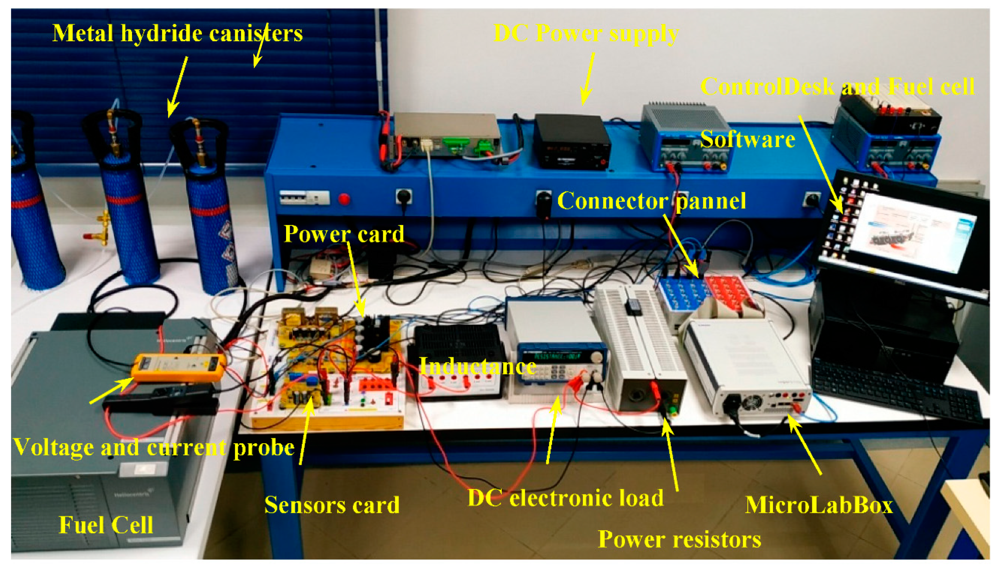
The experimental test bench of the association comprising a 1.2 kW PEMFC fuel cell linked to DC-DC converters is developed and the control system is implemented using MicrolabBox-DSPACE DS1202 to confirm the theoretical analysis.

The remainder of this paper is organized as follows. In Section 2, presentation, modeling, and analysis of the association of a PEMFC and DC-DC power converters are described. A robust controller design and stability analysis is presented in Section 3. Section 4 is devoted to simulation results. Section 5 recapitulates the contributions and confirms theoretical results by experimentation. A conclusion and references list end the paper.

2. Fuel Cell and DC-DC Power Converters—Presentation, Modeling and Analysis

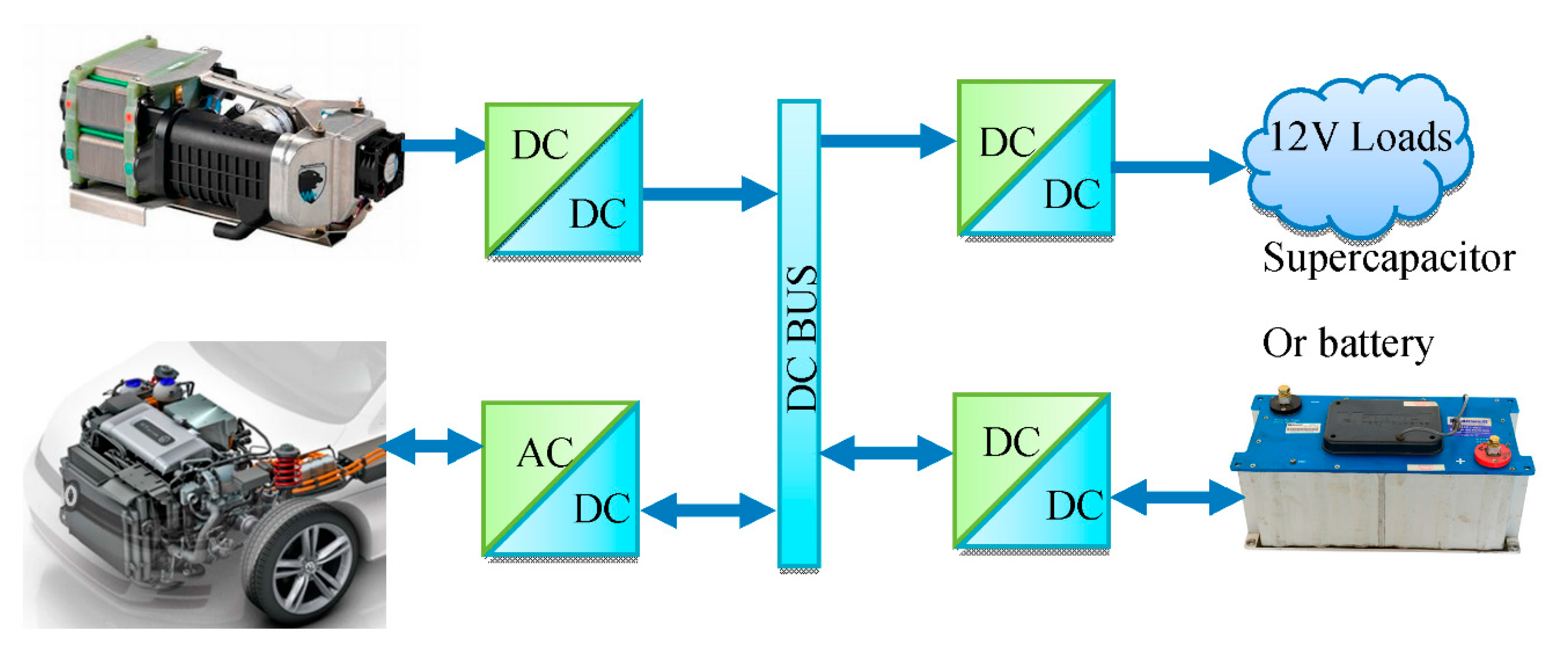
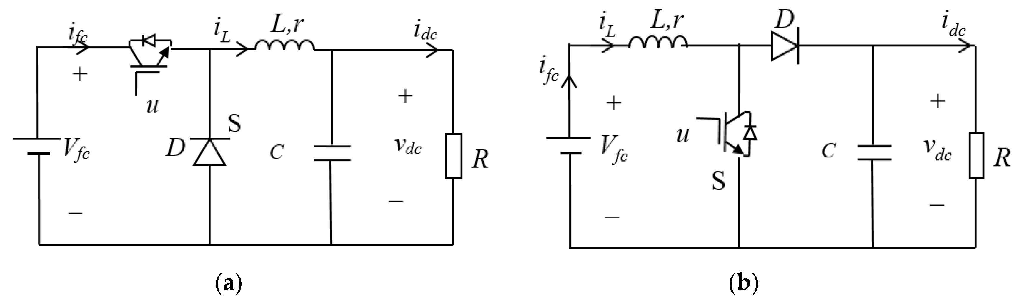
2.1. DC-DC Power Converters Presentation

Boost and buck DC-DC power converters are basic power electronic circuits, and have been widely used in the fields of DC power supplies and DC motor speed regulating systems [26]. Figure 1 shows typical pulse wide modulation (PWM)-based DC-DC converter structures of buck and boost types, where i_L is the inductance current; v_dc the dc bus voltage; L the filtering inductance; C the filtering capacitor; r the inductance ESR; R the load resistance representing the DC bus impedance, which may vary; V_fc the fuel cell voltage; and u the switching binary input signal. Each of these models involves passive components that are subject to linear laws.

Remark 1. 

It should be noted that the resistance R in Figure 2 is a fictive resistance that represents the current consumed by all of the loads connected to the dc bus:$i_{dc}=\frac{v_{dc}}{R}$.

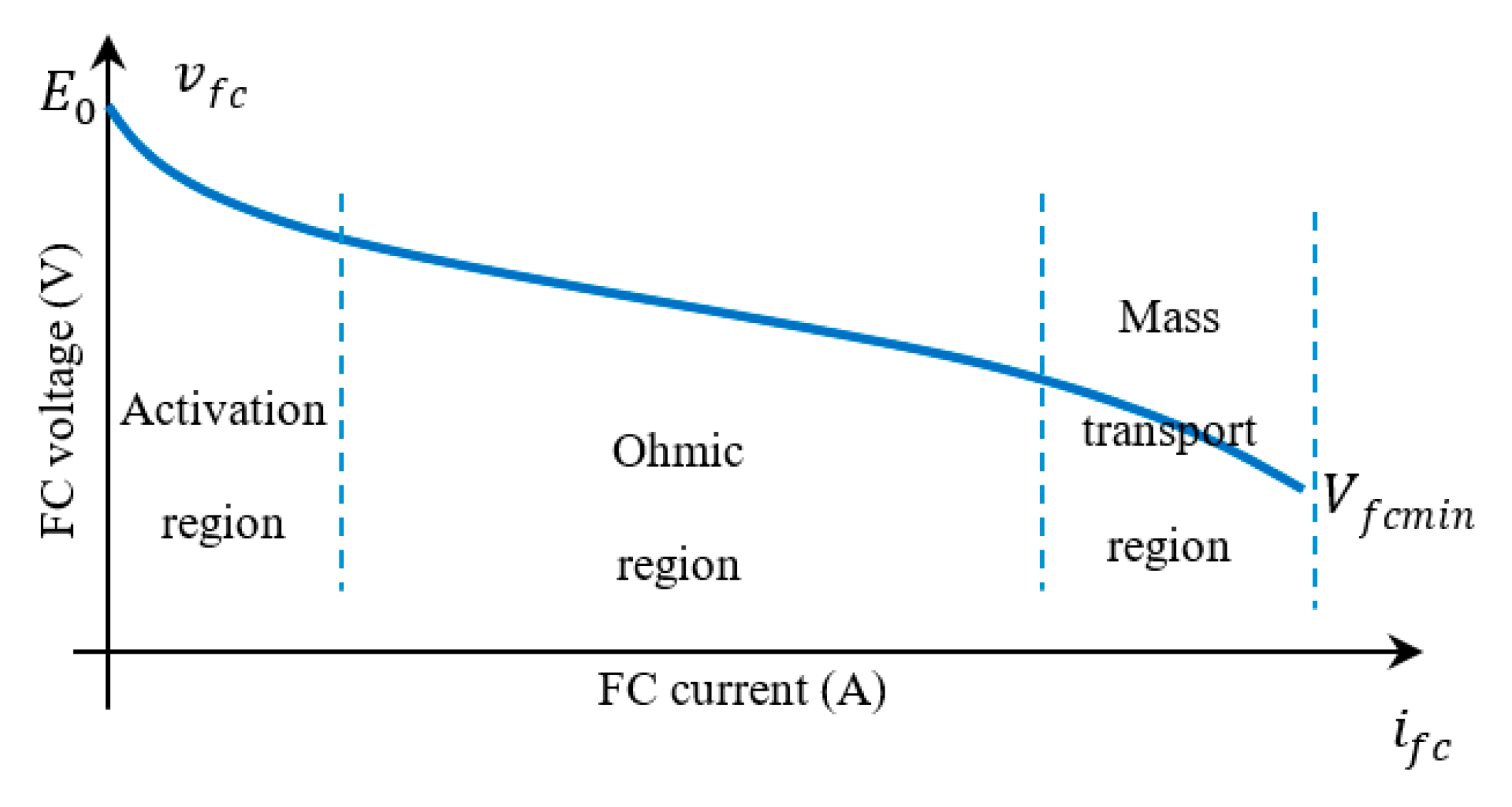
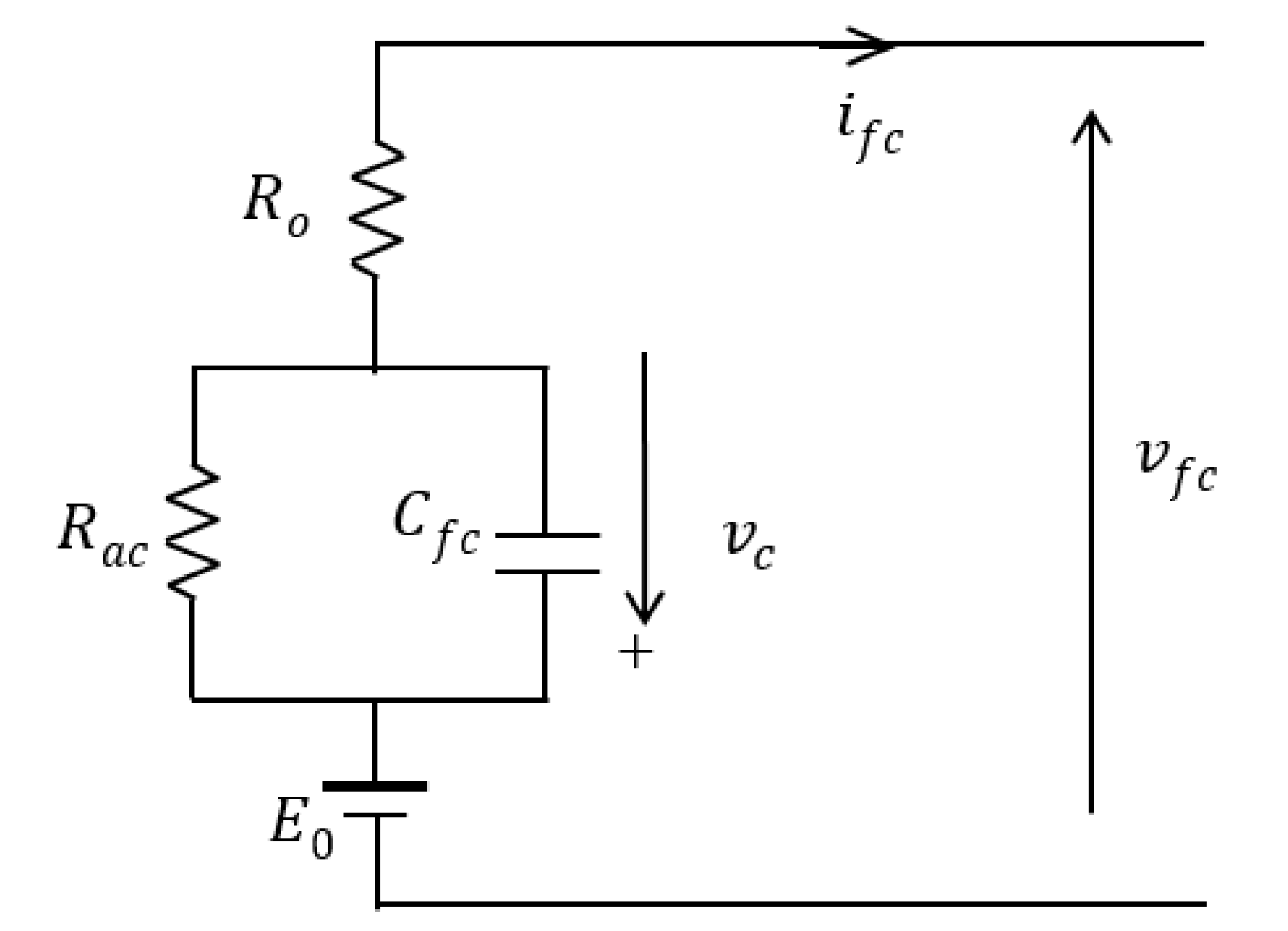
2.2. Fuel Cell Modeling

In this work we consider the static (current-voltage) characteristic of the PEMFC, as shown in Figure 3. This nonlinear characteristic [27] depends on the thermodynamically predicted fuel cell voltage output and three major losses: activation losses (due to electrochemical reaction), ohmic losses (due to ionic electronic condition), and concentration losses (due to mass transport). To take into account the FC dynamics, an equivalent electric circuit illustrated by Figure 4 is used [28].

Then, the FC voltage is governed by the following equations:

$$v_{fc}=E_0-R_o{i}_{fc}-v_c$$

(1)

$$\frac{d{v}_c}{dt}=-\frac{1}{{\tau }_{fc}}{v}_c+\frac{1}{C_{fc}}{i}_{fc}$$

(2)

where $E_0$ is the open circuit voltage, $R_o$ is the ohmic resistance, $C_{fc}$ is the equivalent electrical capacitance, ${\tau }_{fc}=C_{fc}{R}_{ac}$ is the fuel cell electrical time constant, and $R_{ac}$ represents the series equivalent resistance of the activation and concentration resistances.

2.3. Modeling and Analysis of the FC-Buck System

From inspection of the circuit shown in Figure 2a and the circuit of Figure 4, and taking into account that u can take the binary values 1 or 0 and that $i_{fc}=u\times i_L$ and $u\times i_{fc}=u\times i_L$, the following bilinear switching model of the buck converter associated with the FC is obtained:

$$\frac{d{i}_L}{dt}=-\frac{\left(r+u{R}_o\right)}{L}{i}_L-\frac{1}{L}{v}_{dc}+u\frac{\left(E_0-v_c\right)}{L}$$

(3)

$$\frac{d{v}_{dc}}{dt}=\frac{1}{C}{i}_L-\frac{1}{RC}{v}_{dc}$$

(4)

$$\frac{d{v}_c}{dt}=u\frac{1}{C_{fc}}{i}_L-\frac{1}{{\tau }_{fc}}{v}_c$$

(5)

For control design purposes, using the averaging technique [29], the following averaged nonlinear model is obtained:

$$\frac{d{x}_1}{dt}=-\frac{\left(r+\mu R_o\right)}{L}{x}_1-\frac{1}{L}{x}_2+\mu \frac{\left(E_0-x_3\right)}{L}$$

(6)

$$\frac{d{x}_2}{dt}=\frac{1}{C}{x}_1-\frac{1}{RC}{x}_2$$

(7)

$$\frac{d{x}_3}{dt}=\mu \frac{1}{C_{fc}}{x}_1-\frac{1}{{\tau }_{fc}}{x}_3$$

(8)

where $x_1$,$x_2$, and x₃ denote, respectively, the average input current (i_L), the average output capacitor voltage (v_dc), and the average FC internal voltage, and µ is the duty ratio function μ ∈ [0, 1] of the PWM signal which acts as the control input for the above model.

The control objective of the buck converter is to regulate the output voltage to a desired value, e.g., $x_{20}=V_d$, then the operating point ($x_{10}, x_{20}, x_{30}, {\mu }_0$) is defined as follows:

$$x_{20}=V_d$$

(9)

$$x_{10}=I_d=\frac{V_d}{R}$$

(10)

$$x_{30}={\mu }_0{R}_{ac}{I}_d=\frac{{\mu }_0{R}_{ac}{V}_d}{R}$$

(11)

$$\frac{R_{ac}}{R}{\mu }_0^2-\left(\frac{E_0}{V_d}-\frac{R_o}{R}\right){\mu }_0+1+\frac{r}{R}=0$$

(12)

Equation (12) shows that there exists an equilibrium point for the FC-buck system if the following condition holds:

$$g\left(R\right)={\left(\frac{E_0}{V_d}-\frac{R_o}{R}\right)}^2-4\frac{R_{ac}}{R}\left(1+\frac{r}{R}\right)>0$$

(13)

This clearly means that, for a given fuel cell and a desired output voltage $V_d<V_{fcmin}$ (see Figure 3), the load resistance R to be fed by the fuel cell should be carefully chosen. Indeed, the study of the function g(R) represented in (13) leads to examination of the following two cases:

Case 1:$R_o^2<4\times r\times R_{ac}$; the plot of g(R) is illustrated in Figure 5 and represented by the curve (a). It follows that (13) is fulfilled if the load resistance is chosen as follows:

$$R>R_{min1}=\frac{2\left(4r{R}_{ac}-R_o^2\right)}{-\left(2R_o\left(\frac{E_0}{V_d}\right)+4R_{ac}\right)+\sqrt{\mathsf{\Delta }}}$$

(14)

$$\mathsf{\Delta }=16R_{ac}\left[R_{ac}+\left(\frac{E_0}{V_d}\right)\left(R_o+\left(\frac{E_0}{V_d}\right)r\right)\right]>0$$

(15)

Case 2:$R_o^2>4\times r\times R_{ac}$; the plot of $g\left(R\right)$ is illustrated in Figure 5 and represented by the curve (b). Then (13) is fulfilled if the load resistance R is chosen as follows:

$$R>R_{min2}=\frac{2\left(R_o^2-4r{R}_{ac}\right)}{2R_o\left(\frac{E_0}{V_d}\right)+4R_{ac}-\sqrt{\mathsf{\Delta }}}$$

(16)

The minimum of curve b in Figure 5 is obtained for a load resistance R_min obtained as follows:

$$R=R_{min}=\frac{2\left(R_o^2-4r{R}_{ac}\right)}{2R_o\left(\frac{E_0}{V_d}\right)+4R_{ac}}$$

(17)

This gives the following corresponding coordinate:

$$g_{min}=-\frac{\mathsf{\Delta }}{4\left(R_o^2>4\times r\times R_{ac}\right)}<0$$

(18)

It should be emphasized that the second condition to fulfill (13) in case 2 is not of interest because it leads to choosing a load resistance $R<R_{max2}$ which does not have practical interest.

Let us now consider that the condition (13) is fulfilled; then, the meaningful equilibrium point of the duty ratio ${\mu }_0$, using (10), is obtained as follows:

$${\mu }_0=\frac{\left(\frac{E_0}{V_d}-\frac{R_o}{R}\right)-\sqrt{{\left(\frac{E_0}{V_d}-\frac{R_o}{R}\right)}^2-4\frac{R_{ac}}{R}\left(1+\frac{r}{R}\right)}}{2\frac{R_{ac}}{R}}$$

(19)

Now, for linear control it is desirable to establish a transfer function of the system. This is obtained by linearizing the non-linear model (6)–(8) around its operating point. Considering small variations around the operating point ($x_1={\tilde{x}}_1+x_{10}, x_2={\tilde{x}}_2+x_{20},x_3={\tilde{x}}_3+x_{30}, \mu =\tilde{\mu }+ {\mu }_0$), it follows from (6)–(8), using (9)–(12), that the linearized model is obtained as:

$$\frac{d{\tilde{x}}_1}{dt}=-\frac{\left(r+{\mu }_0{R}_o\right)}{L}{\tilde{x}}_1-\frac{1}{L}{\tilde{x}}_2-\frac{{\mu }_0}{L}{\tilde{x}}_3+\frac{\left(E_0-x_{30}-R_o{x}_{10}\right)}{L}\tilde{\mu }$$

(20)

$$\frac{d{\tilde{x}}_2}{dt}=\frac{1}{C}{\tilde{x}}_1-\frac{1}{RC}{\tilde{x}}_2$$

(21)

$$\frac{d{\tilde{x}}_3}{dt}=\frac{{\mu }_0}{C_{fc}}{\tilde{x}}_1-\frac{1}{{\tau }_{fc}}{\tilde{x}}_3+\frac{x_{10}}{C_{fc}}\tilde{\mu }$$

(22)

Note that all cross quantities (${\tilde{x}}_i\tilde{\mu }$) are neglected because we consider small variations. Taking into account that the controlled signal of the buck converter is the DCbus voltage ($y\left(t\right)=x_2\left(t\right)$), and using Laplace transform of (20) and (21), the following transfer function is obtained:

$$G_1\left(s\right)=\frac{{\tilde{x}}_2\left(s\right)}{\tilde{\mu }\left(s\right)}=\frac{b_{11}s+b_{10}}{a_{13}{s}^3+a_{12}{s}^2+a_{11}s+a_{10}}$$

(23)

where

$$b_{11}=(E_0-x_{30}-R_o{x}_{10}) R_{ac}{C}_{fc}$$

(24)

$$b_{10}=E_0-x_{30}-(R_o+{\mu }_0{R}_{ac})x_{10}$$

(25)

$$a_{13}=R_{ac}{C}_{fc}LC$$

(26)

$$a_{12}=LC+\left(\frac{L}{R}+\left(r+{\mu }_0{R}_o\right)C\right)R_{ac}{C}_{fc}$$

(27)

$$a_{11}=\frac{L}{R}+\left(r+{\mu }_0{R}_o\right)C+R_{ac}\left[{\mu }_0^{2}C+\left(1+\frac{r+{\mu }_0{R}_o}{R}\right)C_{fc}\right]$$

(28)

$$a_{10}=1+\frac{r+{\mu }_0{R}_o}{R}+{\mu }_0^2\frac{R_{ac}}{R}$$

(29)

wheres is the Laplace operator.

The main result of this subsection is summarized in the following Proposition.

Proposition 1. 

Consider the fuel cell and buck converter association represented in Figure 2a and Figure 4. A nonlinear averaged model of the association is given by (6)–(8) and its transfer function obtained by linearizing is given by (23). Given a desired value of the output voltage$V_d<V_{fcmin}$, then the equilibrium point of the system is represented by (9)–(11) and (9) provided that the condition (13) is fulfilled. The study of condition (13) shows that the load resistance R should be correctly chosen according to the situations given by (14) and (16).

2.4. Modeling and Analysis of the FC-Boost System

Using the same notations of the previous subsection, the following instantaneous model of the DC-DC boost converter associated with the fuel cell is obtained as follows:

$$\frac{d{i}_L}{dt}=-\frac{\left(r+R_o\right)}{L}{i}_L-\frac{\left(1-u\right)}{L}{v}_{dc}-\frac{1}{L}{v}_c+\frac{E_0}{L}$$

(30)

$$\frac{d{v}_{dc}}{dt} =\frac{\left(1-u\right)}{C}{i}_L-\frac{1}{RC}{v}_{dc}$$

(31)

$$\frac{d{v}_c}{dt}=\frac{1}{C_{fc}}{i}_L-\frac{1}{{\tau }_{fc}}{v}_c$$

(32)

Again, using the average technique [29], the following averaged model is obtained:

$$\frac{d{x}_1}{dt}=-\frac{\left(r+R_o\right)}{L}{x}_1-\frac{\left(1-\mu \right)}{L}{x}_2-\frac{1}{L}{x}_3+\frac{E_0}{L}$$

(33)

$$\frac{d{x}_2}{dt}=\frac{\left(1-\mu \right)}{C}{x}_1-\frac{1}{RC}{x}_2$$

(34)

$$\frac{d{x}_3}{dt}=\frac{1}{C_{fc}}{x}_1-\frac{1}{{\tau }_{fc}}{x}_3$$

(35)

The control objective of the DC-DC boost converter is to regulate the output voltage to a desired value$x_{20}=V_d$; the relationships between different variables in steady state are given by the following:

$$x_{20}=V_d$$

(36)

$$x_{10}=I_d=\frac{V_d}{R\left(1-{\mu }_0\right)}$$

(37)

$$x_{30}=R_{ac}{I}_d=\frac{R_{ac}{V}_d}{R}$$

(38)

$${\left(1-{\mu }_0\right)}^2-\left(1-{\mu }_0\right)\frac{E_0}{V_d}+\frac{r+R_o+R_{ac}}{R}=0$$

(39)

Solving equation (39) gives:

$${\mu }_0=1-\frac{1}{2}\left(\frac{E_0}{V_d}+\sqrt{{\left(\frac{E_0}{V_d}\right)}^2-4\left(\frac{r+R_o+R_{ac}}{R}\right)}\right)$$

(40)

and (37) becomes:

$$x_{10}=I_d=\frac{2V_d^2}{R{E}_0\left(1+\sqrt{1-4\left(\frac{r+R_o+R_{ac}}{R}\right)\frac{V_d^2}{E_0^2}}\right)}$$

(41)

It is worth noting that (16) exist if the following condition holds:

$${\left(\frac{E_0}{V_d}\right)}^2-4\left(\frac{r+R_o+R_{ac}}{R}\right)>0$$

(42)

This means that, in the presence of the inductance ESR r and the FC ohmic resistance Ro, it is not always possible to guarantee the desired output voltage $V_d$ or to supply any load. Indeed, the following two cases should be accounted for:

Case 1: The load resistance R is constant and known, then the output desired voltage should be chosen to be lower than the following maximum value:

$$V_d<V_{dmax}=\frac{E_0}{2\sqrt{\frac{r+R_o+R_{ac}}{R}}}$$

(43)

Case 2: The desired output voltage $V_d$ is constant and known, then the load resistance to be fed should be chosen to be greater than the following minimum value:

$$R>R_{min}=4{\left(\frac{V_d}{E_0}\right)}^2\left(r+R_o+R_{ac}\right)$$

(44)

Now, let us determine a transfer function of the FC-boost association represented by its nonlinear model (33)–(35) useful for control purposes. Consider small variations around the operating point given by (36)–(41) $x_1={\tilde{x}}_1+x_{10}, x_2={\tilde{x}}_2+x_{20},x_1={\tilde{x}}_3+x_{30}, \mu =\tilde{\mu }+{\mu }_0$; then, (33)–(35) gives:

$$\frac{d{\tilde{x}}_1}{dt}=-\frac{\left(r+R_o\right)}{L}{\tilde{x}}_1-\frac{\left(1-{\mu }_0\right)}{L}{\tilde{x}}_2-\frac{1}{L}{\tilde{x}}_3+\frac{x_{20}}{L}\tilde{\mu }$$

(45)

$$\frac{d{\tilde{x}}_2}{dt}=\frac{\left(1-{\mu }_0\right)}{C}{\tilde{x}}_1-\frac{1}{RC}{\tilde{x}}_2-\frac{x_{10}}{C}\tilde{\mu }$$

(46)

$$\frac{d{\tilde{x}}_3}{dt}=\frac{1}{C_{fc}}{\tilde{x}}_1-\frac{1}{{\tau }_{fc}}{\tilde{x}}_3$$

(47)

Note that the cross quantities (${\tilde{x}}_2\tilde{\mu }\mathrm{and}{\tilde{x}}_1\tilde{\mu }$) in (45) and (46) are neglected because we consider small variations (small signal model).

In addition, it is well known that the boost converter presents a no minimum phase feature. This means that the output voltage cannot be regulated directly. Particularly, only the zero dynamics with respect to the inductor current x₁ are stable, which implies that the output voltage of the boost converter should be indirectly controlled via the regulation of the inductor current x₁ to its desired value given by (41) [30]. It follows that the transfer function of interest for the boost converter is that representing the behavior of the system with the duty ratio as an input and the inductor current as the output. From (45)–(47), using Laplace transform, we then obtain:

$$G_2\left(s\right)=\frac{{\tilde{x}}_1\left(s\right)}{\tilde{\mu }\left(s\right)}=\frac{b_{22}{s}^2+b_{21}s+b_{20}}{a_{23}{s}^3+a_{22}{s}^2+a_{21}s+a_{20}}$$

(48)

where

$$b_{22}=R_{ac}{C}_{fc}C{x}_{20}$$

(49)

$$b_{21}=C{x}_{20}+R_{ac}{C}_{fc}\left(\frac{x_{20}}{R}+\left(1-{\mu }_0\right)x_{10}\right)$$

(50)

$$b_{20}=\frac{x_{20}}{R}+\left(1-{\mu }_0\right)x_{10}$$

(51)

$$a_{23}=R_{ac}{C}_{fc}LC$$

(52)

$$a_{22}=LC+\left(\frac{L}{R}+\left(r+R_o\right)C\right)R_{ac}{C}_{fc}$$

(53)

$$a_{21}=\frac{L}{R}+\left(r+R_o\right)C+R_{ac}\left[C+\left({\left(1-{\mu }_0\right)}^2+\frac{r+R_o}{R}\right)C_{fc}\right]$$

(54)

$$a_{20}={\left(1-{\mu }_0\right)}^2+\frac{r+R_o+R_{ac}}{R}$$

(55)

The main result of this subsection is summarized in the following Proposition:

Proposition 2. 

Consider the fuel cell and boost converter association represented in Figure 2b and Figure 4. A nonlinear averaged model of the association is given by (33)–(35) and its transfer function obtained by linearizing is given by (48). Given a desired value of the output voltage$V_d>0$, then the equilibrium point of the system is represented by (36)–(38) and (40) provided that the condition (42) is fulfilled. The study of condition (42) shows that the load resistance R and the desired output voltage$V_d>0$should be correctly chosen according to the situations given by (43) and (44).

The next section is devoted to the design of a robust PID controller of (59) bearing in mind the fact that μ(t) is constrained between 0 and 1. In the sequel we will consider that the transfer function G(s) = y(s)/μ(s), representing a linear model of DC-DC power converter associated with the fuel cell, is represented as follows:

$$G\left(s\right)=\frac{B\left(s\right)}{A\left(s\right)}=\frac{b_2{s}^2+b_{1}s+b_0}{s^3+a_2{s}^2+a_{1}s+a_0}$$

(56)

where

$$B\left(s\right)=b_2{s}^2+b_{1}s+b_0$$

(57)

$$A\left(s\right)=s^3+a_2{s}^2+a_{1}s+a_0$$

(58)

where$y=x_2$ represents the buck converter, $y=x_1$ the boost converter, and all parameters are listed in

Table 1. Parameters involved in (56–58).

Parameter	Buck Converter	Boost Converter
$b_0$	$\frac{1}{R_{ac}{C}_{fc}LC}\left[E_0-x_{30}-(R_o+{\mu }_0{R}_{ac})x_{10}\right]$	$\frac{1}{R_{ac}{C}_{fc}LC}\left[\frac{x_{20}}{R}+\left(1-{\mu }_0\right)x_{10}\right]$
$b_1$	$\frac{1}{LC}(E_0-x_{30}-R_o{x}_{10})$	$\frac{1}{R_{ac}{C}_{fc}L}{x}_{20}+\frac{1}{LC}\left(\frac{x_{20}}{R}+\left(1-{\mu }_0\right)x_{10}\right)$
$b_2$	0	$\frac{1}{L}{x}_{20}$
$a_0$	$\frac{1}{R_{ac}{C}_{fc}LC}\left(1+\frac{r+{\mu }_0{R}_o+{\mu }_0^2{R}_{ac}}{R}\right)$	$\frac{1}{R_{ac}{C}_{fc}LC}\left[{\left(1-{\mu }_0\right)}^2+\frac{r+R_o+R_{ac}}{R}\right]$
$a_1$	$\frac{1}{R_{ac}{C}_{fc}}\left[\frac{1}{RC}+\frac{\left(r+{\mu }_0{R}_o\right)}{L}\right]+\frac{1}{LC}\left[1+{\mu }_0^2\frac{C}{C_{fc}}+\frac{r+{\mu }_0{R}_o}{R}\right]$	$\frac{1}{R_{ac}{C}_{fc}}\left(\frac{1}{RC}+\frac{\left(r+R_o\right)}{L}\right)+\frac{1}{LC}\left({\left(1-{\mu }_0\right)}^2+\frac{C}{C_{fc}}+\frac{r+R_o}{R}\right)$
$a_2$	$\frac{1}{RC}+\frac{1}{R_{ac}{C}_{fc}}+\frac{\left(r+{\mu }_0{R}_o\right)}{L}$	$\frac{1}{RC}+\frac{1}{R_{ac}{C}_{fc}}+\frac{\left(r+R_o\right)}{L}$

.

Proposition 3. 

The polynomial$A\left(s\right)$in (58) representing the denominator of the transfer function of the association consisting of a fuel cell and a DC-DC converter is always Hurwitz regardless of the parameters of the system.

Proof. 

Because all coefficients$a_i \left(i=0,\dots ,2\right)$ are positive (see Table 1), using Routh criterion,$A\left(s\right)$ is Hurwitz if $a_1\times a_2>a_0$. From Table 1, we can easily show that $a_1\times a_2=a_0+\beta$, where $\beta$ is a positive term (which can be easily determined). It follows that $a_1\times a_2>a_0$, which means that$A\left(s\right)$ is Hurwitz. This property is useful for the stability analysis of the saturated controller undertaken later in this paper. □

To take into account the parameter uncertainties (uncertainties of the fuel cell nonlinear characteristic and the load), we suppose hereafter that the output of the converter is affected by a perturbation w(t).

$$y\left(t\right)=\frac{B\left(s\right)}{A\left(s\right)}\mu \left(t\right)+w\left(t\right)$$

(59)

The perturbation is supposed to not be accessible to measurement but to be bounded and slowly varying in the sense that:

$$sw\left(t\right)\in L_2\left(\left[0,+\infty \right]\right)$$

(60)

This perturbation can represent, practically speaking, all modeling errors or parameter uncertainties (such as the load resistance variations).

3. Controller Design and Stability Analysis

3.1. PID Controller with Anti-Windup

The objective now is to design a controller that regulates the output voltage of a DC-DC power converter associated with the fuel cell, represented by (56)–(59). To this end, the following PID controller can be used:

$$C\left(s\right)=K_p+K_i\frac{1}{s}+K_d\frac{{\omega }_{d}s}{s+{\omega }_d}=\frac{S\left(s\right)}{s\left(s+{\omega }_d\right)}$$

(61)

where

$$S\left(s\right)=s_2{s}^2+s_{1}s+s_0$$

(62)

$$s_2=K_p+K_d{\omega }_d$$

(63)

$$s_1=K_p{\omega }_d+K_i$$

(64)

$$s_0=K_i{\omega }_d$$

(65)

where K_p, K_i, and K_d are the proportional gain, the integral gain, and the derivative gain, respectively, and ${\omega }_d$ is the cut-off frequency of the “derivative filter”.

Although many aspects of a control system can be understood based on linear theory, some nonlinear effects must be accounted for in practice. In fact, the “windup” phenomenon is one aspect that appears when a digital controller is implemented for systems with constrained input [31].

The deterioration of the controller performance (when the system deviates from its nominal operation point) is presently worsened by the presence of the control input limitation (the duty ratio is constrained between 0 and 1). The presence of both input limitation and an integrator in the controller cause the closed-loop system to suffer from what is commonly called the “windup effect”. This means that the system signals are likely to diverge if a disturbance affects the system. Presently, the disturbance is produced by the modeling error resulting from the load resistance and the fuel cell characteristic uncertainties.

To overcome this issue, a PID controller with “anti-windup” is used (see Figure 4) instead of the classical structure (61).

Integrator windup is avoided due to back-calculation which works as follows: when the output saturates, the integral term in the controller is recomputed so that its new value gives an output at the saturation limit. It is advantageous not to reset the integrator instantaneously but dynamically with a time constant $T_i=1/K_s$. The time constant T_s determines how quickly the integrator of the PI controller is reset.

According to Figure 6a, the following saturated linear PID controller is used:

$$v=\left(K_p+K_i\frac{1}{s}+K_d\frac{{\omega }_{d}s}{s+{\omega }_d}\right)e_t\left(t\right)+\frac{K_s}{s}{e}_s\left(t\right)$$

(66)

$$\mu =sat\left(v\right)$$

(67)

$$e_s=\mu -v$$

(68)

$$e_t=y_r-y$$

(69)

where$e_t$ is the output tracking error and y_r is the output reference signal supposed to be bounded and slowly varying in the sense that:

$$s{y}_r\left(t\right)\in L_2\left(\left[0,+\infty \right]\right)0<y_r<\frac{b_0}{a_0}$$

(70)

and sat(.) denotes the (non-symmetrical) saturation function defined by:

$$sat\left(v\right)=\{\begin{array}{c}1\hspace{1em} if\hspace{1em} v>1\\ v if 0\le v\le 1\\ 0\hspace{1em} if\hspace{1em} v<1\end{array}$$

(71)

Many design techniques may be used to obtain the controller parameters in (66). Specifically, all linear design methods can be used, e.g., pole-placement and linear-quadratic [32]. For the sake of simplicity, let us consider the pole placement technique. Accordingly, the above operators are uniquely obtained by solving the following Bezout equation:

$$sA\left(s\right)R\left(s\right)+B\left(s\right)S\left(s\right)=P\left(s\right)F\left(s\right)=D\left(s\right)$$

(72)

where

$$R\left(s\right)=s+{\omega }_d$$

(73)

and

$$P\left(s\right)=s^3+p_2{s}^2+p_{1}s+p_0$$

(74)

$$F\left(s\right)=s^2+f_{1}s+f_0$$

(75)

are Hurwitz polynomials ($p_i>0$ and $f_i>0$, $i=0,1$, and $p_2{p}_1-p_0>0$) whose choice will be subject to conditions specified later, and the characteristic polynomial is given by the following:

$$F\left(s\right)=s^5+d_4{s}^4+d_3{s}^3+d_2{s}^2+d_{1}s+d_0$$

(76)

3.2. Tracking Performance Achievement

In this section, the tracking capability of the saturated regulator defined by Equations (66)–(69), when applied to the constrained and perturbed system (59), is analyzed. Operating $sA\left(s\right)$ on (69) and using (59) gives the following fictive system:

$$sA\left(s\right)e_t=-B\left(s\right)\left(s\mu \right)-A\left(s\right)\left(sw\right)+A\left(s\right)(s{y}_r)$$

(77)

Furthermore, operating s on (66), using (61), (68) and (73), one obtains:

$$sv=\frac{S\left(s\right)}{R\left(s\right)}{e}_t+K_s\left(\mu -v\right)$$

which becomes:

$$v=\frac{S\left(s\right)}{R\left(s\right)\left(s+K_s\right)}{e}_t+\frac{K_s}{\left(s+K_s\right)}\mu$$

(78)

Taking the polynomial F(s) in (72) as follows:

$$F\left(s\right)=R\left(s\right)\left(s+K_s\right)=\left(s+{\omega }_d\right)\left(s+K_s\right)$$

(79)

allows us to write:

$$\frac{K_s}{\left(s+K_s\right)}=1-\frac{sR\left(s\right)}{F\left(s\right)}$$

(80)

Equation (78) becomes, using (79) and (80):

$$v=\frac{S\left(s\right)}{F\left(s\right)}{e}_t+\left(1-\frac{sR\left(s\right)}{F\left(s\right)}\right)\mu$$

(81)

This equation in conjunction with (67) represents the constrained controller which we analyze hereafter.

Combining (77) with (81) to eliminate $e_t$, using (72), yields:

$$sv=-\left(\frac{P\left(s\right)-A\left(s\right)}{A\left(s\right)}\right)s\mu +\frac{S\left(s\right)}{F\left(s\right)}\left(s{y}_r-sw\right)$$

(82)

Equation (82), combined with the fact that $=sat\left(v\right)$, leads to the feedback representation of Figure 6a, with:

$$H\left(s\right)=\frac{P\left(s\right)-A\left(s\right)}{A\left(s\right)}$$

(83)

$${\xi }_1\left(t\right)=\frac{S\left(s\right)}{F\left(s\right)}\left(s{y}_r\left(t\right)-sw\left(t\right)\right)$$

(84)

where $\varphi$ is a (nonlinear) operator that maps $sv$ into $s\mu$, and which is found to belong to the sector $\left[0,1\right]$, (see [22,33]) in the sense that:

$$0\le \left(s\mu \right)\left(sv\right)\le {\left(sv\right)}^2$$

(85)

Theorem 1. 

We consider a system whose input–output relationship is represented by y = Hu where H is some mapping or operator that specifies y in terms of u. Input u belongs to a space of signals that map the time interval [0,$\infty$) into the Euclidean space$R^m$. The definition of$L_2$-stability is the familiar notion of boundedinput–bounded output stability; namely, if the system is$L_2$-stable therefore every bounded input u(t), the output Hu(t) is bounded.

Proposition 4. 

Let the polynomial$P\left(s\right)$, in (74) be chosen Hurwitz so that:

$$\underset{0\le \omega <+\infty }{\inf }\mathrm{Re}\left(\frac{P\left(j\omega \right)}{A\left(j\omega \right)}\right)>0$$

(86)

If the reference signal y_r(t) is any bounded signal so that (70) holds and w(t) is any bounded disturbance satisfying (60), then the feedback of Figure 7 is L₂-stable and, consequently:

(1) 

$s\mu \in L_2$,$sv \in L_2$,$s{e}_t \in L_2$,$sy \in L_2$

(2) 

$\left(v-\mu \right)\in L_2$

(3) 

$e_t \in L_2$

Proof. 

Because F(s) belongs to the sector $\varphi$ and satisfies the positive real property (86), it follows from the circle criterion [34] that the feedback of Figure 7 is L₂-stable, Furthermore, because $F\left(s\right)$ is Hurwitz and $\frac{S\left(s\right)}{F\left(s\right) }$ is a proper transfer function, from (70) and (60) it follows that:

$${\xi }_1\left(t\right)\in L_2$$

(87)

Then, all internal signals of the feedback Figure 7 belong to $L_2$ which means that:

$$s\mu \in L_2,sv \in L_2$$

(88)

Proposition 3 shows that the polynomial $A\left(s\right)$ is Hurwitz; thus, it follows from (77), (70), (60) and (88) that:

$$s{e}_t \in L_2$$

(89)

Furthermore, from (69) one gets $sy=s{e}_t+s{y}_r$, which together with (70) gives:

$$sy \in L_2$$

(90)

In view of (62), (81) can be rewritten as follows:

$$v-\mu =\frac{s_{2}s+s_1}{F\left(s\right)}(s{e}_t)-\frac{R\left(s\right)}{F\left(s\right)}\left(s\mu \right)+\frac{s_0}{F\left(s\right)}{e}_t$$

(91)

Because $F\left(s\right)$ is Hurwitz and $\frac{sB\left(s\right)}{A\left(s\right)}$ is a proper transfer function and using the fact that $0<y_r<\frac{b_0}{a_0}$, it is shown [22] using (91) that:

$$\left|v-\mu \right|\le \left|{\xi }_2\left(t\right)\right|$$

(92)

where${\xi }_2\left(t\right)$ is a L₂-stable signal (${\xi }_1\left(t\right)\in L_2)$. It follows that:

$$\left(v-\mu \right)\in L_2$$

(93)

Let us operate $R\left(s\right)$on both sides of (77) and $F\left(s\right)\times B\left(s\right)$ on both sides of (81); then, one gets, successively:

$$sAR{e}_t=-BR\left(s\mu \right)+AR\left(s{y}_r-sw\right)$$

(94)

$$BF\left(v-\mu \right)=BS{e}_t-BR\left(s\mu \right)$$

(95)

Combining (94) and (95), using (72) one obtains:

$$e_t=\frac{B}{P}\left(v-\mu \right)-\frac{AR}{PF}\left(s{y}_r-sw\right)$$

(96)

Because the transfer functions $\frac{B}{P}$ and $\frac{AR}{PF}$ are L₂-stable, $\left(v-\mu \right)\in L_2$,$s{y}_r\in L_2$ and $sw\in L_2$, it follows that:

$$e_t\in L_2$$

(97)

□

This establishes Proposition 4.

This proposition gives us, indeed, the basic elements with which to formulate the main result of this section, i.e., the tracking objective and the fact that the control signal stops saturating asymptotically. This is properly formulated in the following theorem.

Theorem 2. 

Consider the closed-loop system represented by Figure 6a and composed of:

(1) 

The constrained system (59) modeling the fuel cell and DC-DC converter association, where w(t) is any bounded disturbance satisfying (60).

(2) 

The saturated controller (66) and (67), where the reference$y_r$is any bounded reference signal ($0<y_r<\frac{b_0}{a_0}$) satisfying (70), and ($P\left(s\right)$and$F\left(s\right)$) are any Hurwitz polynomials of the form (74) and (75). If the operator$P\left(s\right)$satisfies the real positive condition (86), then, the tracking error$e_t\left(t\right)$and the deviation$v\left(t\right)-\mu \left(t\right)$between the computed and the applied controls both vanish asymptotically

Proof. 

From (97) and (89) we have $e_t \in L_2$ and $\in L_2$. It follows, using Barbalat’s Lemma, that $e_t\left(t\right)$ converges exponentially to zero. In addition, from (92) and (88), we have $\left(v-\mu \right)\in L_2$ and $s\left(\mu -v\right) \in L_2$; it follows, again using Barbalat’s Lemma, that $v\left(t\right)-\mu \left(t\right)$ exponentially vanishes. The theorem is then established. □

3.3. Practical Considerations for Determining PID Parameters

In practice, to satisfy the real positive condition (86), an appropriate choice of the polynomials $P\left(s\right)$ and $F\left(s\right)$consists of using the following general rules [22]:

$$P\left(s\right)=A\left(s+{\lambda }_1\right) \mathrm{with}{\lambda }_1\ge 0$$

(98)

$$F\left(s\right)=A\left(s+{\lambda }_2\right) \mathrm{with}{\lambda }_2\ge {\lambda }_1$$

(99)

Note that Equation (99) could be used if the polynomials $F\left(s\right)$ and $A\left(s\right)$have the same degree. Otherwise (this is our case) we choose the zeros of $F\left(s\right)$to be real but preferably faster than the regulation (zerosof $P\left(s\right)$).

In view of (74) and (79), the parameters of the characteristic polynomial $D\left(s\right)$ are obtained as follows:

$$d_0=p_0{\omega }_d{K}_s$$

(100)

$$d_1=p_1{\omega }_d{K}_s+p_0({\omega }_d+K_s)$$

(101)

$$d_2=p_0+p_1({\omega }_d+K_s)+p_2{\omega }_d{K}_s$$

(102)

$$d_3=p_1+p_2({\omega }_d+K_s)+{\omega }_d{K}_s$$

(103)

$$d_4=p_2+{\omega }_d+K_s$$

(104)

In addition, solving the Bezout Equation (72), using (57), (58), (62), (65) and (73)–(76), gives:

$$b_0{s}_0=d_0$$

(105)

$$a_0{\omega }_d+b_1{s}_0+b_0{s}_1=d_1$$

(106)

$$a_0+a_1{\omega }_d+b_2{s}_0+b_1{s}_1+b_0{s}_2=d_2$$

(107)

$$a_1+a_2{\omega }_d+b_2{s}_1+b_1{s}_2=d_3$$

(108)

$$a_2+{\omega }_d+b_2{s}_2=d_4$$

(109)

Now, combining (100)–(109), we obtain the following nonlinear equation system with unknown variables $\left(s_0,s_1, s_2,{\omega }_d, K_s\right)$ subject to constraints: ${\omega }_d>0$ and $K_s>0$:

$$b_0{s}_0-p_0{\omega }_d{K}_s=0$$

(110)

$$b_1{s}_0+b_0{s}_1+\left(a_0-p_0\right){\omega }_d-p_0{K}_s-p_1{\omega }_d{K}_s=0$$

(111)

$$b_2{s}_0+b_1{s}_1+b_0{s}_2+\left(a_1-p_1\right){\omega }_d-p_1{K}_s-p_2{\omega }_d{K}_s+a_0-p_0=0$$

(112)

$$b_2{s}_1+b_1{s}_2+\left(a_2-p_2\right){\omega }_d-p_2{K}_s-{\omega }_d{K}_s+a_1-p_1=0$$

(113)

$$b_2{s}_2-K_s+a_2-p_2=0$$

(114)

The procedure for determining the controller parameters can be summarized as follows:

(1)

Chose the polynomial$P\left(s\right)$ to ensure (86).

(2)

Solve a system (110)–(114) to obtain $\left(s_0,s_1, s_2,{\omega }_d, K_s\right)$, ensure that ${\omega }_d>0$ and $K_s>0$, else return to (1) to modify $P\left(s\right)$.

(3)

Using (62)–(64), determine the parameters$K_i$, $K_p$ and $K_d$ of the PID controller as follows:$K_i=\frac{s_0}{{\omega }_d}$,$K_p=\frac{s_1-K_i}{{\omega }_d}$; $K_d=\frac{s_2-K_p}{{\omega }_d}$.

The next section is devoted to validating the proposed approach and analysis by numerical simulation.

4. Simulation Results

4.1. System Parameters

According to Figure 6, which describes the system under study, and using the instantaneous models of power converters (buck and boost) defined respectively by (3)–(5) and (30)–(32), the system was simulated using MATLAB/Simulink.

The fuel cell parameters used in the simulation are the real parameters of the Ballard Nexa 1200 fuel cell module which has a rated power of 1.2 kW. All parameters are listed in

Table 2. Controlled system parameters: fuel cell and DC-DC converter.

	Parameter Designation	Value
Fuel Cell	FC open circuit voltage	$E_0=28.3 \mathrm{V}$
	FC internal capacitor	$C_{fc}=130 \mathrm{F}$
	Association of the activation and concentration resistances	$R_{ac}=0.155 \mathsf{\Omega }$
	Ohmic resistance	$R_O=2.89 \mathrm{m}\mathsf{\Omega }$
DC-DC Converter	Filtering inductance	$L=4 \mathrm{mH}$
	Filtering capacitor	$C=680 \mathsf{\mu }\mathrm{F}$
	ESR of the inductance	$r=0.2 \mathsf{\Omega }$
	load nominal value	$R=10 \mathsf{\Omega }$
	PWM switching frequency	$f_s=20 \mathrm{kHz}$

.

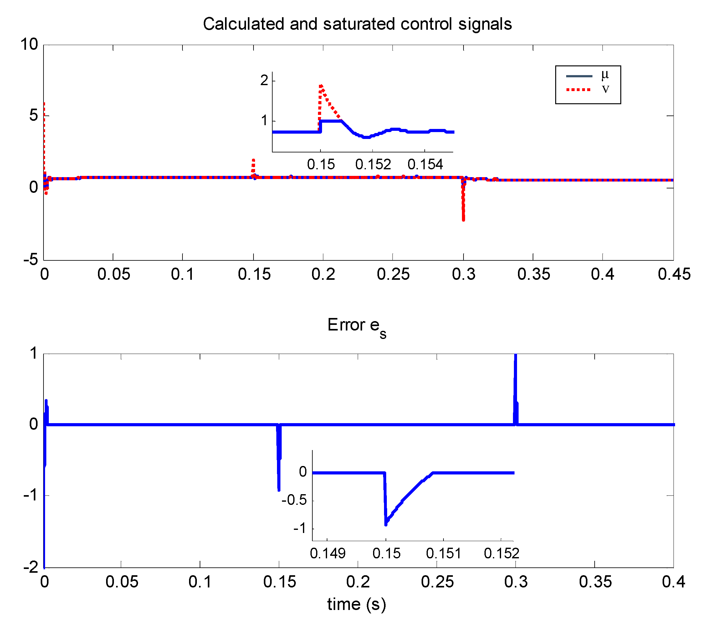
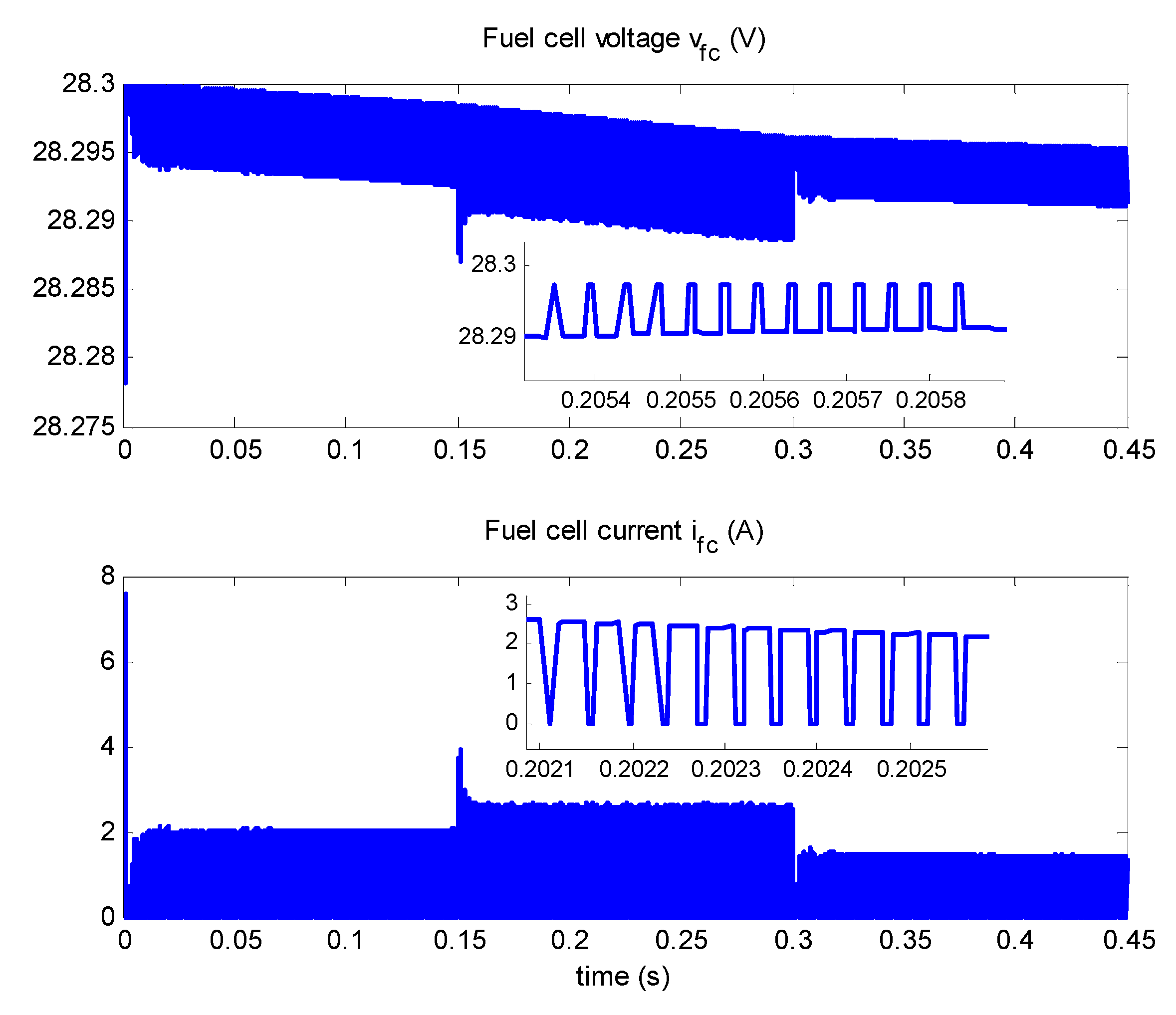
4.2. Simulation of the FC-Buck Association

Using the parameters listed in Table 1 and Table 2, the transfer function of the association consisting of the fuel cell and buck power converter was simulated using MATLAB/Simulink. Equations (110)–(114) were solved using solve function of MATLAB. The parameters of the controller were then obtained. The transfer function and the parameter design of the controller are summarized in

Table 3. Transfer function and controller parameters for the Fuel Cell-Buck system.

Transfer Function $G\left(s\right)$	$G\left(s\right)=\frac{1.028\times {10}^{7}s+5.043\times {10}^5}{s^3+197.7s^2+3.751\times {10}^{5}s+1.883\times {10}^4}$
Controller	$K_p=0.0618$
	$K_i=5.2478$
	$K_d=1.295\times {10}^{-4}$
	${\omega }_d=1830.3\left(rad/s\right)$
	$K_s=0.049$

. The obtained controller was then applied to the instantaneous model (3)–(5) (which actually represents the system) instead of the linearized model which is only used to design the controller. The simulation bench is illustrated by Figure 6. The controller performance is shown in Figure 8, Figure 9, Figure 10 and Figure 11.

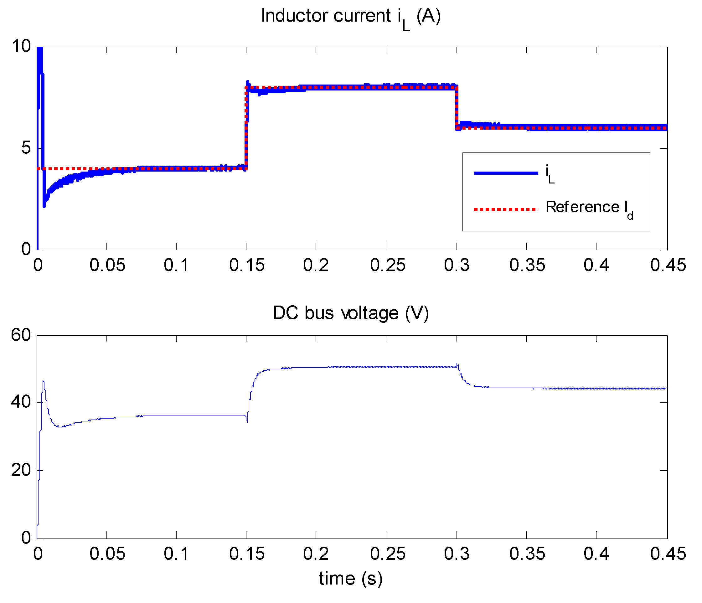
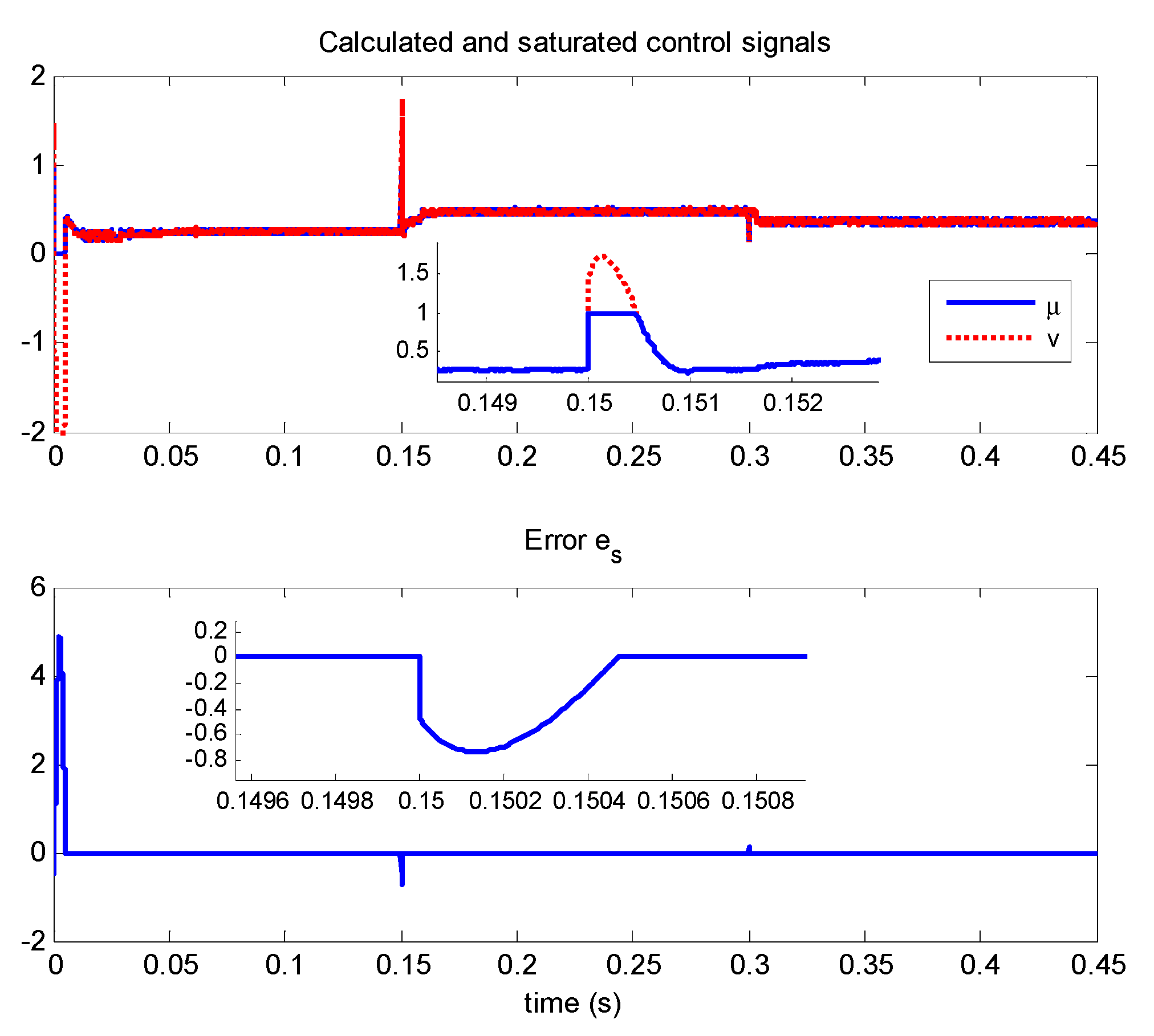
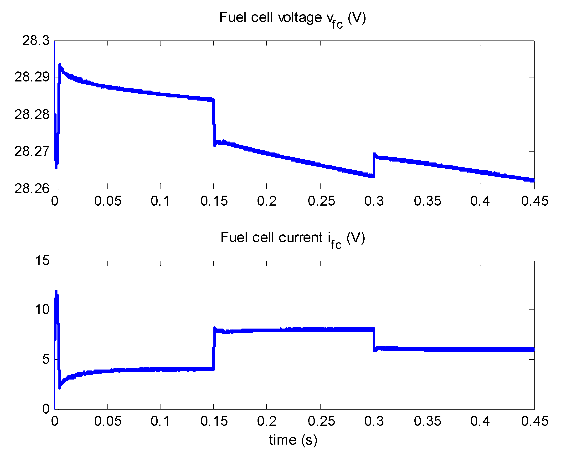
4.2.1. Controller Behavior in the Presence of Output Reference Variations

Figure 8 illustrates the closed-loop behavior in ideal conditions (no model uncertainty: the load resistance is set constant $=10 \mathsf{\Omega }$) when the reference trajectory of the DC bus voltage is a signal switching from 20 V to 24 V at instant 0.15 s and returns to 14 V at instant 0.3 s. It is clearly seen that the DC bus voltage $v_{dc}$ perfectly tracks its reference after the transient time (following the reference signal changes). Figure 9 shows the computed and applied control signals,$v\left(t\right)$ and $\mu \left(t\right)$. It is seen that $\mu \left(t\right)$ tracks $v\left(t\right)$ after a finite transient period. That is, the controller stops saturating after these time intervals, confirming thus the theoretical results of the proposed theorem. Figure 10 shows the fuel cell voltage and current behavior in the presence of a time-varying reference. From this figure one can see that the fuel cell voltage varies, however, despite these variations the output voltage is perfectly regulated to its reference.

In addition, the figure shows a pulsating current which can be harmful for the fuel cell. Indeed, the PEMFC is very sensitive to current ripples, which limit the fuel cell lifetime and reduce its efficiency [35].

This section is divided into subheadings. These provide a concise and precise description of the experimental results and their interpretation, in addition to the experimental conclusions that can be drawn.

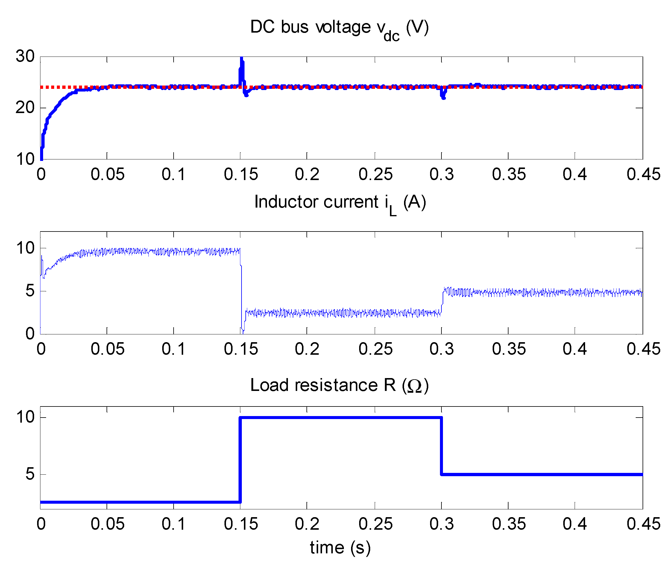
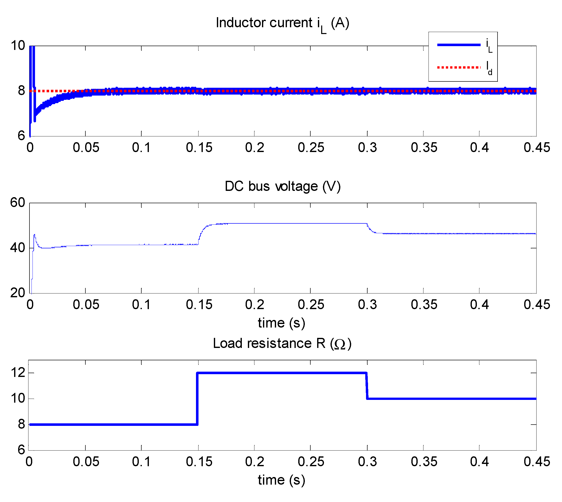
4.2.2. Controller Sensitivity to the Perturbation Caused by Load Uncertainty

In practical situations the load resistance that represents the consumed current of all loads connected to the DC bus perpetually changes, although its value may not be precisely known. Note that these features are accounted for in the control model (59) by the presence of a perturbation signal $w\left(t\right)$. It is seen, from a theoretical point of view, that the saturated controller in (66) and (67) is robust with respect to such a perturbation. This aspect is also confirmed by simulations. Figure 11 and Figure 12 illustrate the response of the closed-loop system to a reference step of 24 V, in the presence of load resistance changes. Specifically, the load switches from 2.5 Ω to 10 Ω at instant 0.15 s and returns to 5 Ω at instant 0.3 s. Even in the presence of these disturbances, Figure 11 shows a good tracking performance, whereas Figure 12 shows that during the transient mode the control system is saturated. In fact, the magnified view of this signal shows explicitly that the control signal is no longer saturated after each transient mode.

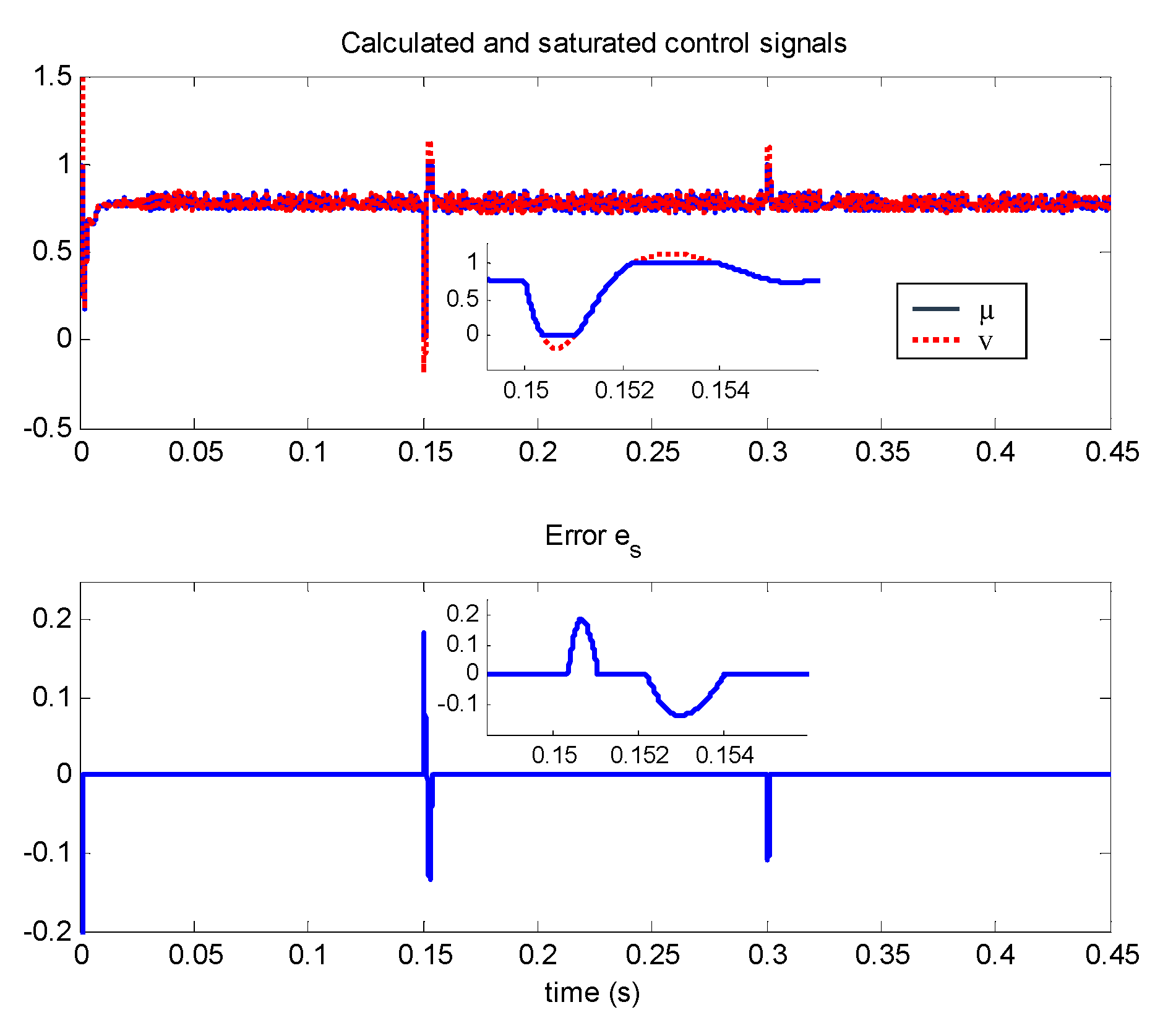
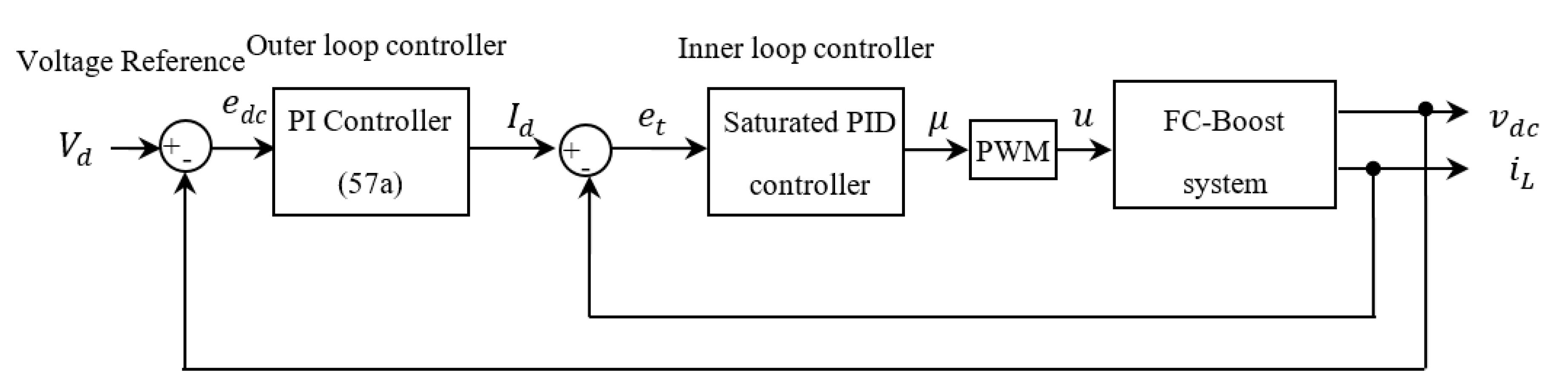
4.3. Simulation of the FC-Boost Association

Given the values of Table 2, the limits of the reference voltage $V_d$ and the load resistance $R$ given, respectively, by the Equations (43) and (44) are obtained as follows: $V_{dmax}=74.8 V$,$R_{min}=4.12 \mathsf{\Omega }$ (for $V_d=48 V$). The transfer function of the association FC-boost and the parameters of the controller obtained by solving Equations (110)–(114) are summarized in

Table 4. Transfer function and controller parameters for the fuel cell-boost system.

Transfer Function $G\left(s\right)$	$G\left(s\right)=\frac{12\times {10}^3{s}^2+3.53\times {10}^{6}s+1.752\times {10}^5}{s^3+197.8s^2+1.072\times {10}^{5}s+5603}$
Controller	$K_p=0.58586$
	$K_i=29.0857$
	$K_d=-4.9557\times {10}^{-5}$
	${\omega }_d=5649.8634\left(rad/s\right)$
	$K_s=2.03$

.

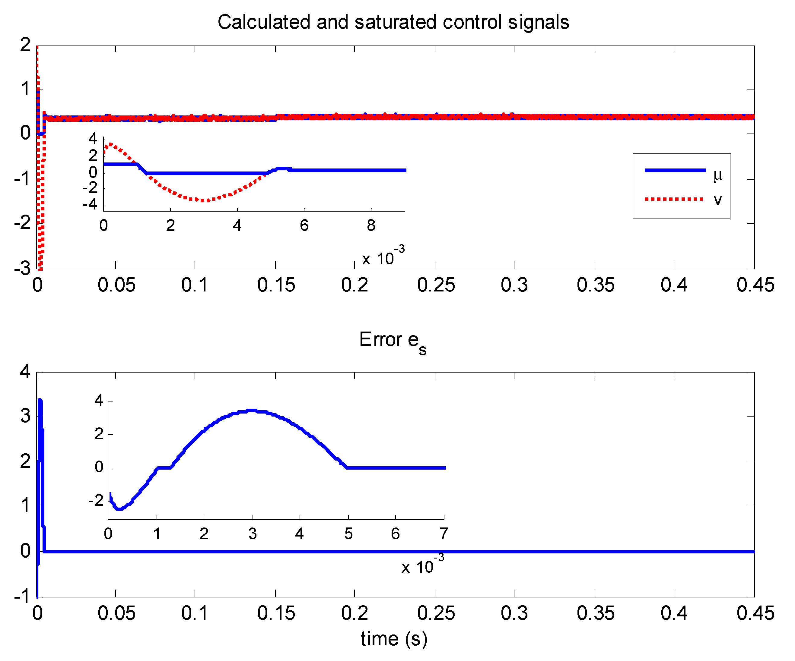
4.3.1. Validation of the Performances of the Current Loop (Inner Loop)

For the boost converter, the controller shown in Figure 6 is designed to regulate the inductor current to its desired value. In this section we validate the performances of this controller (often called the internal loop or current loop controller) in terms of tracking and stopping the saturation effect after a transient as shown by the theoretical result given by theorem. The DC bus voltage regulation is illustrated in the next subsection.

(A)

Controller behavior in the presence of output reference variations:

Figure 13, Figure 14 and Figure 15 illustrate the closed-loop behavior in the presence of step changes of the reference trajectory of the inductor current when the load resistance is set constant at $R=12 \mathsf{\Omega }$. Precisely, the current reference $I_d$ is a signal switching from 4 A to 8 A at instant 0.15 s and returning to 6 A at instant 0.3 s. It is clearly seen from Figure 13 that the inductor current $i_L$ perfectly tracks its reference after a transient time (following the reference signal changes). Figure 14 shows that the error $e_s\left(t\right)$ between the computed and applied control signals vanishes, which confirms the theoretical results of the theorem and shows that the controller stops saturating after a time interval. Figure 15 shows the fuel cell voltage and current. A non-pulsating current of the fuel cell with a small ripple is evident, which proves that the boost converter is better suited to interface with fuel cells. The continuous input-current feature of the boost converter contributes to maintaining the life-time of the fuel cell, which is in sharp contrast with the buck converter whose input current damages the fuel cell and reduces the efficiency.

(B)

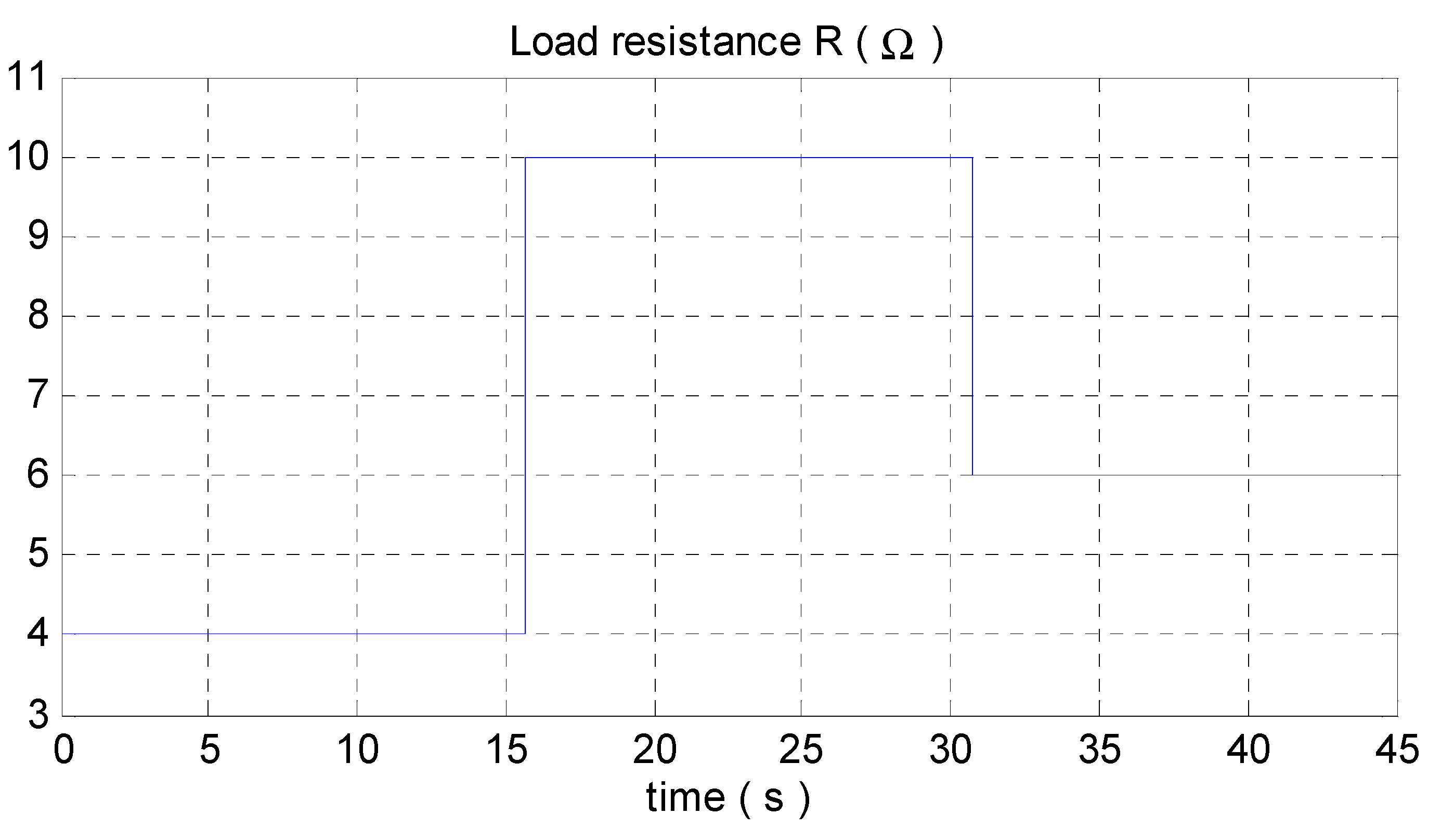
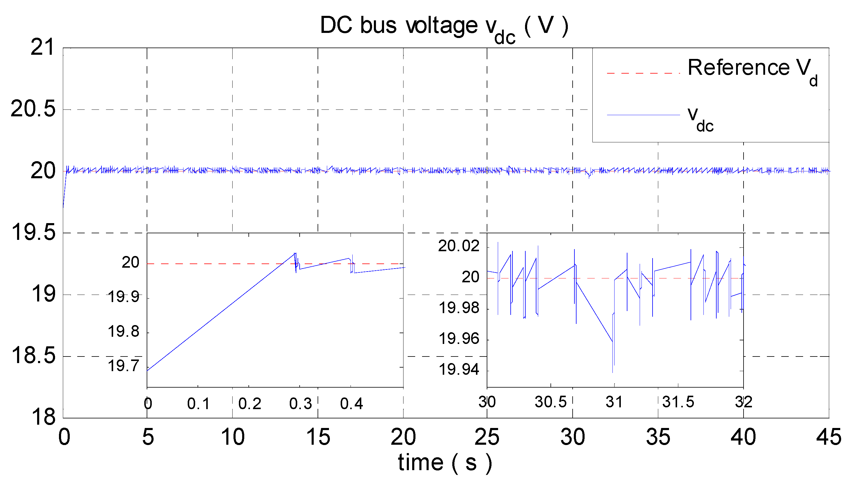
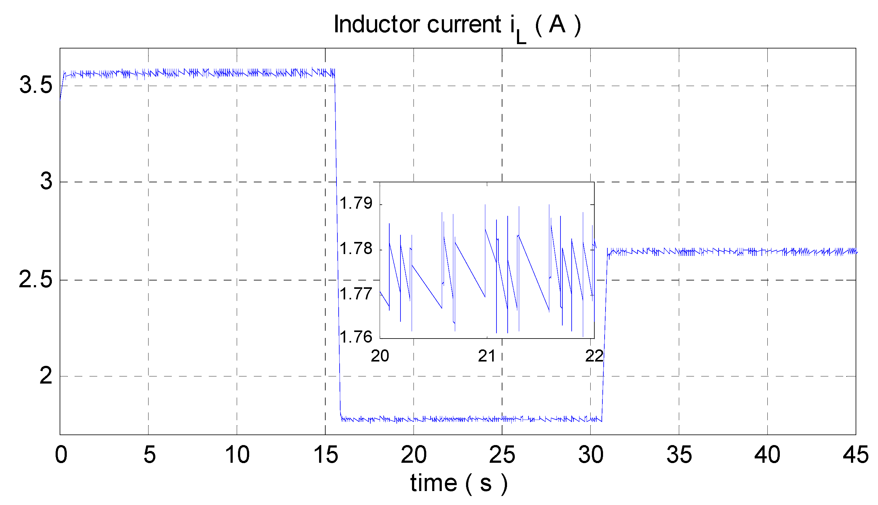
Controller sensitivity to the perturbation caused by load uncertainty.

Figure 16 and Figure 17 illustrate the response of the closed-loop system to a reference step of 8 A, in the presence of load resistance changes. Specifically, the load switches from 8 Ω to 12 Ω at instant 0.15 s and returns to 10 Ω at instant 0.3 s. Even in the presence of load variations the controller ensures a good tracking performance and stops saturating after a transient time, as illustrated by Figure 16 and Figure 17.

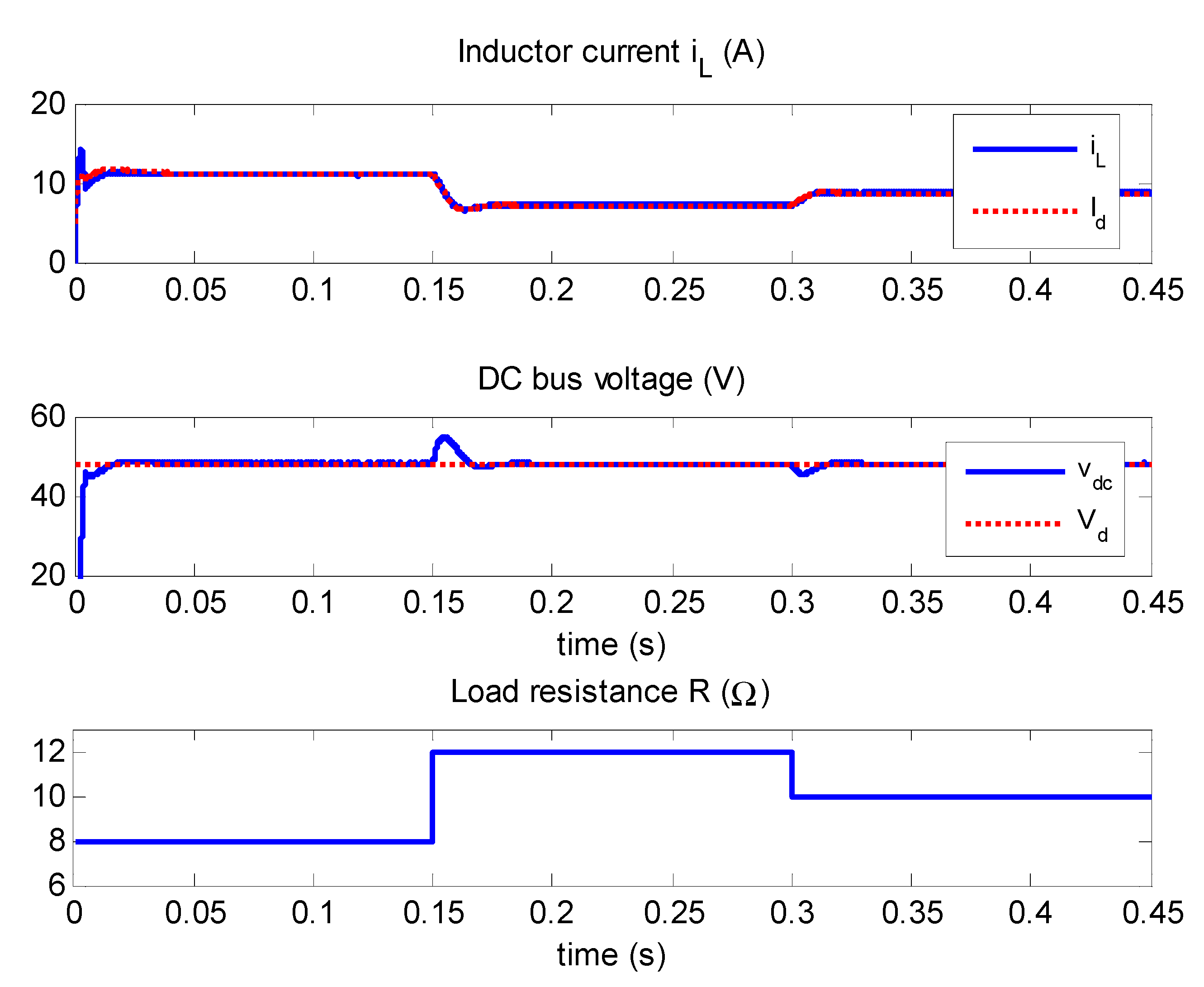
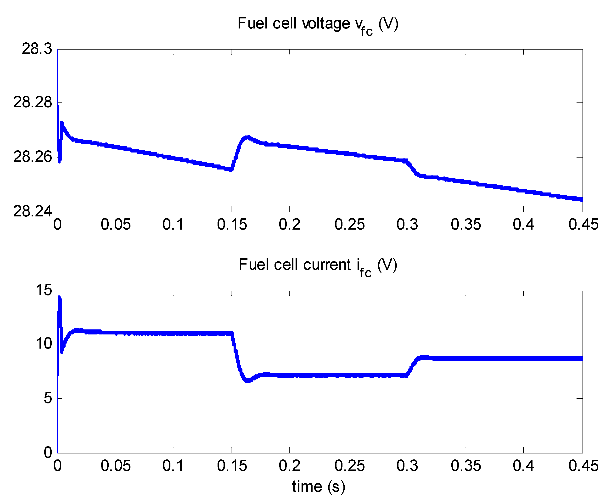
4.3.2. Validation of the Performances of the Voltage Loop (Outer Loop)

In the last subsection we clearly showed that the inner loop controller ensures that the inductor current perfectly tracks its reference and the controller stops saturating after a transient time as shown by the theorem. Nevertheless, the controller is not sufficient to ensure a DC bus voltage regulation. Indeed, in the presence of load resistance variations, the output voltage is not regulated at all. To achieve this objective an outer loop (voltage loop) is performed as illustrated in Figure 18. To determine the outer loop controller, the transfer function representing the behavior of the DC bus voltage $v_{dc}$ with respect to the inductor current $i_L$ must be established. Operating the Laplace transform on the linearized model (91)–(93), the following transfer function is obtained:

$$G_3\left(s\right)=\frac{{\tilde{x}}_2}{{\tilde{x}}_1}=-\frac{b_{32}{s}^2+b_{31}s+b_{30}}{\left({\tau }_{fc}s+1\right)\left(\tau s+{\eta }_0\right)}$$

(115)

where

$$b_{32}=LR{\tau }_{fc}\left(\frac{x_{10}}{x_{20}}\right)$$

(116)

$$b_{31}=R\left[L\frac{x_{10}}{x_{20}}+{\tau }_{fc}\left(\frac{x_{10}}{x_{20}}\left(r+R_o\right)-\left(1-{\mu }_0\right)\right)\right]$$

(117)

$$b_{30}=R\left[-\left(1-{\mu }_0\right)+\frac{x_{10}}{x_{20}}\left(r+R_o+R_{ac}\right)\right]$$

(118)

$${\tau }_{fc}=R_{ac}{C}_{fc}$$

(119)

$$\tau =RC$$

(120)

$${\eta }_0=1+\frac{R{x}_{10}}{x_{20}}\left(1-{\mu }_0\right)$$

(121)

The numerical value of the transfer function is obtained as follows:

$$G_3\left(s\right)=\frac{{\tilde{x}}_2}{{\tilde{x}}_1}=-\frac{-0.1547s^2+91.1s+4.522}{\left(20.15s+1\right)\left(6.8\times {10}^{-3}s+2\right)}$$

(122)

For the outer loop a PI controller is simply chosen as:

$$G_3\left(s\right)=K_{pv}+\frac{K_{iv}}{s}$$

(123)

where the parameters were tuned using the PID tuning tool of MATLAB. The following values were obtained, which are tuned to ensure good transient and fast response times:

$$K_{pv}=0.1022; K_{iv}=72.395$$

(124)

Figure 19 illustrates the behavior of the cascade controller structure (consisting of the saturated inner loop PID controller and the outer loop PI controller) for the FC-boost association in the presence of a constant DC bus voltage reference $V_d=48 V$, and load resistance variations. One can see from this figure that, despite load variations, the DC bus voltage is tightly regulated to its desired value. It is worth noting that the obtained tracking performances and robustness against load resistance changes are ensured despite the fuel cell voltage variations as shown in Figure 20.

5. Experimental Results

Figure 21 illustrates the laboratory prototype used for experimental validation. It consists of the Ballard Nexa 1200 fuel cell module, which has a rated power of 1.2 kW, and its monitoring software; three metal hydride canisters from Heliocentris with storage capacities of 800 NL hydrogen; an H2 connection Kit 15 bar to connect the metal canisters; a Hall effect sensors to measure voltage and current variables; a programmable DC electronic load from BK Precision and power resistors to make load changes; a MicroLabBox-dSPACE with Control Desk software plugged into a personal computer for signal acquisition and power and measurement cards. The system parameters are similar to those in Table 4. The technology of dSPACE via MicroLabBox DS 1202 simplified the implementation of the control law via the link between the control Desk^® and MATLAB^®/Simulink^®, to test the systems and measure its quantities (voltage, current). The simulation bench of the fuel cell association with DC-DC power converters controlled by a robust anti-windup PID is shown in Figure 6. The control system was implemented in dSPACE DS1202 via MicroLabBox and used with a real-time interface (RTI). The DS1202 was fully programmable from the Simulink^® block diagram environment, and all inputs/outputs were configured graphically.

Using a programmable DC electronic load, variations of the load resistance were programmed similar to those performed for simulation. The parameters of the control design are listed in

Table 5. Control design parameters.

Parameter	Buck Converter	Boost Converter
kd	10−4	$-4.9557\times {10}^{-5}$
wd	1830.3 rad/s	5649.8634 rad/s
ki	0.9	11
kp	10−3	0.09
ks	0.049	2.03
kpv	-	0.09

, whereas the experiment results of buck and boost power converters are illustrated in Figure 22, Figure 23, Figure 24, Figure 25, Figure 26, Figure 27, Figure 28, Figure 29, Figure 30 and Figure 31.

5.1. Validation of the FC-Buck Association

The resulting performance is illustrated in Figure 22, Figure 23, Figure 24, Figure 25 and Figure 26.

Figure 22 describes the load resistance profile. The load switches from 4 Ω to 10 Ω at instant 15 s and returns to 6 Ω at instant 30 s. Figure 23 shows that, despite load variations, the DCbus voltage ${\mathrm{v}}_{\mathrm{dc}}$ perfectly tracks the reference signal, which is set to $v_d=20\mathrm{V}$. The overshoot at that moment was almost zero. The system response time was around 0.3 s and the DC bus voltage signal ripple was tolerable, with a value of less than 0.06 V due to measurement noise.

Figure 25 shows the fuel cell voltage and current behavior in the presence of a time varying reference. From this figure one can see that the output voltage is perfectly regulated to its reference despite the variations of input voltage, which represent the fuel cell voltage and load variations.

We can note that the obtained tracking performance and robustness against load resistance changes are ensured despite the fuel cell voltage variations shown in Figure 25, which confirms that the controller performance is good.

5.2. Validation of the FC-Boost Association

The load switches from 48 Ω to 96 Ω and returns to 48 Ω. The reference signal of the DC bus voltage is set to $V_d=48 \mathrm{V}$. The resulting performances is illustrated in Figure 27, Figure 28, Figure 29, Figure 30 and Figure 31.

Figure 27 describes the shape of the programmed profile of the load resistance. In Figure 28 we note that the controller ensures the first objective. Indeed, the DCbus voltage $v_c$ perfectly tracks its reference $v_d=48\mathrm{V}$despite load variations. The overshoot at that moment was almost 1.5 V. The system response time was around 0.2 s and the signal ripple was tolerable, at less than 0.06 A due to measurement noise. Figure 29 represents the inductor current, which is a non-pulsating current of the fuel cell with a tolerable ripple (less than 0.02 A). This proves that the boost converter is more convenient to interface with fuel cells. The continuous input-current feature of the boost converter contributes to maintaining the life-time of the fuel cell, which is better than the performance of the buck converter, whose input current damage the fuel cell and reduces the efficiency. We can note that the simulation and experimental results responded perfectly to the theoretical approach used in this paper, namely, perfect tracking performance despite fuel cell and load variations; removing the windup effect and then ensuring closed-loop stability; and short response time.

6. Conclusions

In this study, we present three main contributions. The first contribution addresses the association of the set consisting of a PEMFC and DC-DC converters. A mathematical model of this association for each converter (buck and boost) is elaborated. Secondly, the analysis of the studied system, in particular, the equilibrium point, emphasizes the importance of properly choosing the reference signal of the DC bus voltage and the load resistance to ensure the feasibility of the association. From the simulation and experimental results, we conclude that the DC boost converter is better suited to interface with the fuel cell because of the continuous input current. This feature contributes to protecting and maintaining the life-time of the fuel cell. This is in contrast to the buck converter where it pulsating input current damages the fuel cell and reduces its efficiency in the long term.

Thirdly, a robust PID controller with an anti-windup scheme is proposed and rigorously analyzed. Using absolute stability tools, sufficient conditions are established for the closed-loop system to be L₂-stable. Simulation and experimental results confirm our theoretical analysis and show that the regulator ensures the objectives of closed-loop stability, output reference tracking, and robustness against perturbations. It is important to stress that the modeling, analysis, and design of the controller is performed by taking the fuel cell dynamics and the non-linear characteristic of the fuel cell into account. Indeed, the obtained tracking performance and robustness against load resistance changes are ensured despite variations in the fuel cell voltage.

Finally, we observe that formal analysis, numerical simulations, and experimental results show that the designed robust anti-windup PID controller meets all of the desired objectives.

References

1. Zubi, G.; Dufo-López, R.; Carvalho, M.; Pasaoglu, G. The lithium-ion battery: State of the art and future perspectives. Renew. Sustain. Energy Rev. 2018, 89, 292–308. [Google Scholar] [CrossRef]
2. Kwan, T.H.; Katsushi, F.; Shen, Y.; Yin, S.; Zhang, Y.; Kase, K.; Yao, Q. Comprehensive review of integrating fuel cells to other energy systems for enhanced performance and enabling poly generation. Renew. Sustain. Energy Rev. 2020, 128, 109897. [Google Scholar] [CrossRef]
3. Khaligh, A.; Li, Z. Battery, Ultracapacitor, Fuel Cell, and Hybrid Energy Storage Systems for Electric, Hybrid Electric, Fuel Cell, and Plug-In Hybrid Electric Vehicles. State Art. IEEE Trans. Veh. Technol. 2010, 59, 2806–2814. [Google Scholar] [CrossRef]
4. Ferriz, A.; Bernad, A.; Mori, M.; Fiorot, S. End-of-life of fuel cell and hydrogen products: A state of the art. Int. J. Hydrog. Energy 2019, 44, 12872–12879. [Google Scholar] [CrossRef]
5. Moradisizkoohi, H.; Elsayad, N.; Mohammed, O.A. Experimental Verification of a Double-Input Soft-Switched DC–DC Converter for Fuel Cell Electric Vehicle with Hybrid Energy Storage System. IEEE Trans. Ind. Appl. 2019, 55, 6451–6465. [Google Scholar] [CrossRef]
6. Fathabadi, H. Combining a proton exchange membrane fuel cell (PEMFC) stack with a Li-ion battery to supply the power needs of a hybrid electric vehicle. Renew. Energy 2019, 130, 714–724. [Google Scholar] [CrossRef]
7. Zhang, Y.; Liu, H.; Li, J.; Sumner, M.; Xia, C. DC–DC Boost Converter With a Wide Input Range and High Voltage Gain for Fuel Cell Vehicles. IEEE Trans. Power Electron. 2019, 34, 4100–4111. [Google Scholar] [CrossRef]
8. Kolli, A.; Gaillard, A.; De Bernardinis, A.; Bethoux, O.; Hissel, D.; Khatir, Z. A review on DC/DC converter architectures for power fuel cell applications. Energy Convers. Manag. 2015, 105, 716–730. [Google Scholar] [CrossRef]
9. Kabalo, M.; Blunier, B.; Bouquain, D.; Miraoui, A. State-of-the-art of DC-DC converters for fuel cell vehicles. In Proceedings of the 2010 IEEE Vehicle Power and Propulsion Conference, Lille, France, 1–3 September 2010; pp. 1–6. [Google Scholar]
10. Ahmed, O.; Bleijs, J. An overview of DC–DC converter topologies for fuel cell-ultracapacitor hybrid distribution system. Renew. Sustain. Energy Rev. 2015, 42, 609–626. [Google Scholar] [CrossRef]
11. Daud, W.R.W.; Rosli, R.E.; Majlan, E.H.; Hamid, S.A.A.; Mohamed, R.; Husaini, T. PEM fuel cell system control: A review. Renew. Energy 2017, 113, 620–638. [Google Scholar] [CrossRef]
12. Wang, J.; Zhang, C.; Li, S.; Yang, J.; Li, Q. Finite-Time Output Feedback Control for PWM-Based DC-DC Buck Power Converters of Current Sensorless Mode. IEEE Trans. Control Syst. Technol. 2016, 25, 1359–1371. [Google Scholar] [CrossRef]
13. Ma, R.; Xu, L.; Xie, R.; Zhao, D.; Huangfu, Y.; Gao, F. Advanced Robustness Control of DC–DC Converter for Proton Exchange Membrane Fuel Cell Applications. IEEE Trans. Ind. Appl. 2019, 55, 6389–6400. [Google Scholar] [CrossRef]
14. Zuniga-Ventura, Y.A.; Langarica-Cordoba, D.; Leyva-Ramos, J.; Diaz-Saldierna, L.H.; Ramirez-Rivera, V.M. Adaptive Backstepping Control for a Fuel Cell/Boost Converter System. IEEE J. Emerg. Sel. Top. Power Electron. 2018, 6, 686–695. [Google Scholar] [CrossRef]
15. Huangfu, Y.; Li, Q.; Xu, L.; Ma, R.; Gao, F. Extended State Observer Based Flatness Control for Fuel Cell Output Series Interleaved Boost Converter. IEEE Trans. Ind. Appl. 2019, 55, 6427–6437. [Google Scholar] [CrossRef]
16. Tahri, A.; El Fadil, H.; Rachid, A.; Eric, M.; Giri, F. A Nonlinear Controller Based on a High Gain Observer for a Cascade Boost Converter in a Fuel Cell Distributed Power Supply System. IFAC-PapersOnLine 2019, 52, 91–96. [Google Scholar] [CrossRef]
17. Thounthong, P.; Pierfederici, S. A New Control Law Based on the Differential Flatness Principle for Multiphase Interleaved DC–DC Converter. IEEE Trans. Circuits Syst. II Express Briefs 2010, 57, 903–907. [Google Scholar] [CrossRef]
18. Zumoffen, D.; Basualdo, M. Advanced control for fuel cells connected to a DC/DC converter and an electric motor. Comput. Chem. Eng. 2010, 34, 643–655. [Google Scholar] [CrossRef]
19. Somkun, S.; Sirisamphanwong, C.; Sukchai, S. A DSP-based interleaved boost DC–DC converter for fuel cell applications. Int. J. Hydrog. Energy 2015, 40, 6391–6404. [Google Scholar] [CrossRef]
20. Zhang, Y.; Fu, C.; Sumner, M.; Wang, P. A Wide Input-Voltage Range Quasi-Z-Source Boost DC–DC Converter with High-Voltage Gain for Fuel Cell Vehicles. IEEE Trans. Ind. Electron 2018, 65, 5201–5212. [Google Scholar] [CrossRef] [Green Version]
21. Yang, C.; Sun, J.; Zhang, L. Anti-windup controller design for singularly perturbed systems subject to actuator saturation. IET Control Theory Appl. 2016, 10, 469–476. [Google Scholar] [CrossRef]
22. El Fadil, H.; Giri, F.; Chaoui, F.; El Magueri, O. Accounting for Input Limitation in the Control of Buck Power Converters. IEEE Trans. Circuits Syst. I Regul. Pap. 2009, 56, 1260–1271. [Google Scholar] [CrossRef]
23. Xiao, W.; Wen, H.; Zeineldin, H. Affine parameterization and anti-windup approaches for controlling DC-DC converters. In Proceedings of the 2012 IEEE International Symposium on Industrial Electronics, Hangzhou, China, 28–31 May 2012; pp. 154–159. [Google Scholar]
24. Tarakanath, K.; Patwardhan, S.C.; Agarwal, V. Implementation of an internal model controller with anti-reset windup compensation for output voltage tracking of a non-minimum phase dc-dc boost converter using FPGA. In Proceedings of the 2016 IEEE 2nd Annual Southern Power Electronics Conference (SPEC), Auckland, New Zealand, 5–8 December 2016; pp. 1–6. [Google Scholar]
25. Moreno-Valenzuela, J. A Class of Proportional-Integral With Anti-Windup Controllers for DC–DC Buck Power Converters With Saturating Input. IEEE Trans. Circuits Syst. II Express Briefs 2020, 67, 157–161. [Google Scholar] [CrossRef]
26. KazimierczukMarian, K. Pulse-Width Modulated DC-DC Power Converters, 2nd ed.; Wiley: Hoboken, NJ, USA, 2015. [Google Scholar]
27. Larminie, J. Fuel Cell Systems Explained, 2nd ed.; Wiley: Hoboken, NJ, USA, 2003. [Google Scholar]
28. Wang, C.; Nehrir, M.; Shaw, S.R. Dynamic models and model validation for PEM fuel cells using electrical circuits. IEEE Trans. Energy Convers. 2005, 20, 442–451. [Google Scholar] [CrossRef]
29. Krein, P.; Bentsman, J.; Bass, R.; Lesieutre, B. On the use of averaging for the analysis of power electronic systems. IEEE Trans. Power Electron. 1990, 5, 182–190. [Google Scholar] [CrossRef]
30. El Fadil, H.; Giri, F. Backstepping Based Control of PWM DC-DC Boost Power Converters. In Proceedings of the 2007 IEEE International Symposium on Industrial Electronics, Vigo, Spain, 4–7 June 2007; pp. 395–400. [Google Scholar]
31. Glattfelder, A.H.; Schaufelberger, W. Control Systems with Input and Output Constraints; Springer: Berlin, Germany, 2003. [Google Scholar]
32. Anderson, B.D.O.; Moore, J.B. Optim. Control: Linear Quadratic Methods; Dover Publications: New York, NY, USA, 2007. [Google Scholar]
33. Ghani, D.; Giri, F.; Chater, E.; Chaoui, F.Z.; Haloua, M. Control of Discrete-Time Systems Composed of Linear Blocks in Series with Saturation Components. Asian J. Control 2003, 17, 1935–1945. [Google Scholar] [CrossRef]
34. Khalil, H. Nonlinear Systems Analysis; Prentice Hall, Inc.: Upper Saddle River, NJ, USA, 2003. [Google Scholar]
35. Valdez-Resendiz, J.E.; Sanchez, V.M.; Rosas-Caro, J.C.; Mayo-Maldonado, J.C.; Sierra, J.; Barbosa, R. Continuous input-current buck-boost DC-DC converter for PEM fuel cell applications. Int. J. Hydrog. Energy 2017, 42, 30389–30399. [Google Scholar] [CrossRef]
Figure 1. Power train of a hybrid fuel cell vehicle
Electronics 09 01889 g001
Figure 2. DC-DC buck and boost power converters. (a) Buck converter. (b) Boost converter.
Electronics 09 01889 g002
Figure 3. Nonlinear i-v characteristic of the fuel cell.
Electronics 09 01889 g003
Figure 4. Equivalent electric RC circuit of a fuel cell stack.
Electronics 09 01889 g004
Figure 5. Different plots of the function g(R) of (13). (a,b) represent respectively the curve of g(R) when R o 2 < 4 × r × R a c and R o 2 > 4 × r × R a c .
Electronics 09 01889 g005
Figure 6. (a) PID controller of power converter with anti-windup. (b) Block diagram of the controlled system.
Electronics 09 01889 g006
Figure 7. Nonlinear feedback relating the derivatives of calculated and constrained control signals.
Electronics 09 01889 g007
Figure 8. Tracking behavior of the controller in presence of a time-varying reference signal V d .
Electronics 09 01889 g008
Figure 9. Computed control signal v ( t ) , the applied value   μ ( t ) , and the error e s ( t ) in the presence of a time-varying reference.
Electronics 09 01889 g009
Figure 10. Fuel cell voltage and current in the presence of a time-varying reference.
Electronics 09 01889 g010
Figure 11. Robustness of the saturated controller in the presence of a load resitance uncertainty.
Electronics 09 01889 g011
Figure 12. Computed control signal ( t ) , the applied value μ ( t ) , and the error e s ( t ) in the presence of load resitance uncertainty.
Electronics 09 01889 g012
Figure 13. Tracking behavior of the inner loop controller in the presence of a time-varying reference signal   I d .
Electronics 09 01889 g013
Figure 14. Computed control signal v ( t ) , the applied value μ ( t ) , and the error e s ( t ) in the presence of a time-varying reference.
Electronics 09 01889 g014
Figure 15. Fuel cell voltage and current in the presence of a time-varying reference.
Electronics 09 01889 g015
Figure 16. Robustness of the saturated controller in the presence of load resistance uncertainties.
Electronics 09 01889 g016
Figure 17. Computed control signal v ( t ) , the applied value μ ( t ) , and the error e s ( t ) in presence of resistance load uncertainty.
Electronics 09 01889 g017
Figure 18. Cascade control structure of the FC-boost association.
Electronics 09 01889 g018
Figure 19. Robustness of the cascade controller in the presence of load resistance uncertainties.
Electronics 09 01889 g019
Figure 20. Fuel cell voltage and current in the presence of load resistance changes.
Electronics 09 01889 g020
Figure 21. Laboratory prototype used for experimental validation.
Electronics 09 01889 g021
Figure 22. Programmed profile of the load resistance.
Electronics 09 01889 g022
Figure 23. DCbus voltage V d c .
Electronics 09 01889 g023
Figure 24. Inductance current i L .
Electronics 09 01889 g024
Figure 25. Fuel cell voltage V f c .
Electronics 09 01889 g025
Figure 26. Duty ratio µ.
Electronics 09 01889 g026
Figure 27. Programmed profile of the load resistance.
Electronics 09 01889 g027
Figure 28. DCbus voltage V d c .
Electronics 09 01889 g028
Figure 29. Inductance current i L = i f c .
Electronics 09 01889 g029
Figure 30. Fuel cell voltage V f c .
Electronics 09 01889 g030
Figure 31. Duty ratio µ.
Electronics 09 01889 g031