Development of Surface Drifting Buoys for Fiducial Reference Measurements of Sea-Surface Temperature

Introduction

Sea-Surface Temperatures (SST) play a key role in the understanding of the ocean-atmosphere interactions, in the characterization of the mesoscale variability of the upper ocean, and also as inputs of numerical weather prediction systems. They have traditionally been measured in situ, and since the 1970s, they are also monitored with a global coverage by satellite-borne radiometers (e.g., Prabhakara et al., 1974; Milman and Wilheit, 1985). These instruments measure the radiance emitted by the sea surface. These radiance measurements are sensitive to ocean skin temperature, but are also sensitive to the atmospheric physical state and constituents, and to the sea state. In order to determine more precisely these sources of inaccuracy, methods have been developed to trace radiance measurement uncertainties (Woolliams et al., 2016, 2018; Banks et al., 2017; Merchant et al., 2019). However, to ensure the validity of retrieved SST, comparisons with independent in situ measurements are necessary (O'Carroll et al., 2008). Only after validation, the resulting SST retrievals can be used to generate global datasets with spatio-temporal consistency (e.g., Titchner and Rayner, 2014).

In situ SST measurements go back at least 200 years (Kennedy, 2014). They have been collected for several purposes and with varying instruments. The first measurements were made from seawater collected by buckets, and after by seawater circulating through the steam condenser of the engine room inlets on ships. Since the 1970s, oceanographic and vessels of opportunity are equipped with hull thermometers. In quiet sea states, they measure temperature at 5 or 6 m under the surface and, for the last 10 years, many have been equipped with high-resolution and stable Sea-Bird Electronics (SBE)-38 sensors (e.g., Gaillard et al., 2015). Argo profiling float temperatures are also used for comparisons. Since January 2005, they offer comprehensive ocean coverage (Hausfather et al., 2017). Argo products provide temperatures at different depths: 2.5, 5, 10, 20, 30 m, or deeper levels with an initial accuracy close to 2 mK. Sensors are generally stopped several meters below the surface to avoid the fouling of the conductivity cell by surface contaminants. A few floats are equipped with SBE STS (Surface Temperature Salinity) sensors which sample the final meters up to the surface, with a degraded accuracy in salinity, but most of Argo temperatures exploited as SST are measured at 5 m under the surface (Roemmich and Gilson, 2009). While only the initial accuracy has been guaranteed so far, first efforts have been made to recover Argo floats, in order to document potential changes in trueness (BIPM, 2012) over time (e.g., Oka, 2005).

Generally, measurements made in the upper 10 m of the ocean are considered as SST measurements. However, satellite infrared radiometers measure radiations emitted from the upper few tens of microns (skin temperatures) or millimeters (subskin temperatures) for microwave radiometers (Donlon et al., 2004). Therefore, surface drifting buoys observations are preferred for comparisons with satellites data, as their sensors are at a nominal depth of between 10 and 20 cm (Merchant et al., 2012). According to the Data Buoy Cooperation Panel (DBCP) about 1,500 drifting buoys cover nowadays the seas of the globe and according to (Kennedy, 2014), they provide about 90% of in situ SST data.

Designed in the 1980s to study ocean currents in the context of the Surface Velocity Program (SVP; World Climate Research Programme, 1988) and for meteorological purposes, these buoys had to be inexpensive, easy to deploy and reliable during at least 18 months. The design specifications of SVP drifters were standardized in 1991. In 1993, it became possible to equip a SVP drifter with a barometer port to measure sea-level air pressure. The result was called a SVP-B drifter. SVP drifters were also equipped with SST sensors. This sensor should have an accuracy of 0.1 K with a stability better than 0.1 K/year (World Climate Research Programme, 1988). There were other documented requirements, though less stringent, with 0.5 K requested in the range from −5 to 30°C (EGOS, 2002). Of note in the SVP-B design manual (Sybrandy et al., 2009), is the requirement that a thermal isolation be included to ensure that the solar heating of the top of the surface float does not impact the SST measurement. The sensor should be accurate to better than 0.1 K when the inside of the float is 1 K warmer than the sea surface.

In his publication, Kennedy (2014, Table 2, p. 8) cites 10 references dealing with estimates of measurement errors or uncertainties of drifting buoys (with no clear distinction between error and uncertainty). They range from 0.12 to 0.67 K. He discusses also the possibility to separate observation errors or uncertainties into random and systematic components, particularly for drifters, from two earlier publications (Kennedy et al., 2011a,b) and from a publication by Kent and Berry (2008). They find similar results with estimated random components of (respectively) 0.56 and 0.6 K and systematic components of (respectively) 0.37 and 0.3 K. These values are close, for example, to the expected accuracy of the Advanced Along-Track Scanning Radiometer (AATSR) launched in March 2002. It is designed to produce SST retrievals to better than 0.3 K accuracy, with a long-term stability of better than 0.1 K per decade (Lewellyn-Jones et al., 2001). Therefore, the corresponding drifting buoys SST measurements collected so far cannot be considered as references from a metrological point of view. Neither can they be considered as references for the more recent EUMETSAT-operated Copernicus Sentinel-3A, the first in a new generation of satellites designed to collect and monitor long-term climate and ocean data with metrological specifications equivalent to AATSR (Donlon et al., 2012).

Separating systematic and random components is not an easy task for SST measurements, because the data from several authors (see Kennedy, 2014 or Castro et al., 2012) suggest a dependency on the time period considered. If random components come from the variability in time and space of the thermal and dynamical states of the sea, in the case of SVP drifters, the biggest part of systematic components can come from the buoy and sensor conception and from the unknown temporal drift of their SST sensors.

This short review underlines the need to develop a new concept of surface drifting float which would be characterized in metrology laboratory. Its design has to comply with the requirements of satellite SST measurement validation and must allow the link through comparisons of its measurements to the Système International d'unités (SI). This need was described in a EUMETSAT tender, the goal of which was to build a Fiducial Reference Measurements (FRM) network of 100 high-resolution SST drifting buoys for the Copernicus Sentinel satellites validation. The development of this network echoes also, for the ocean surface, the need raised by Immler et al. (2010) for upper-air measurements, to constitute an independent infrastructure based on a different measurement principle and for which uncertainties are defined. Beyond the needs underlined by the review, this development answers the necessity of assuring long-term stability of references (World Meteorological Organization, 2016), the uncertainties of which are fully characterized by a metrological approach, for climate change studies.

Conception of the Reference Buoys

A drifting buoy with a novel sensor package has been developed, called SVP with Barometer and Reference Sensor for Temperature (SVP-BRST, see Poli et al., 2018). It is a spherical drifter of 40 cm diameter made of high pressure molded polypropylene (see Figure 2). A 12.5 m-long line (including an elastic section) is attached below the buoy and linked to a stainless bracket. A holey sock drogue centered at 15 m depth is suspended to the line. It is 0.8 m in diameter and 6 m in length. The drogue loss is detected by a strain gauge, instead of a submergence sensor (Lumpkin and Pazos, 2006).

A GPS receiver is included in the buoy to provide position estimates, and various GPS quality parameters. The strain gauge reading and the GPS Time To First Fix (TTFF) are transmitted as indicators of drogue loss. The transmission is made hourly, via a 30-bytes iridium Short-Burst Data (SBD) message, in a new dedicated format (Blouch et al., 2018).

The buoy is based on the SVP-B design (Sybrandy et al., 2009). It is equipped with a Vaisala PTB 110 BAROCAP sensor featuring an accuracy of ±0.6 hPa (according to Vaisala documentation) for temperature variations from 0 to 40°C (±0.3 hPa for the temperature range from 15 to 25°C). It is delivered with a NIST traceable calibration certificate. The measurement of SST is made by two sensors: a regular SST sensor with an initial trueness superior to 0.1°C and a new High-Resolution SST sensor called HRSST. As recommended by best-practices, both are protected from solar and buoy radiations by a cap. The regular sensor for SST (called analog sensor thereafter) is made with two cupronickel bolts of diameters 1.4 and 1.9 cm, protecting a 6 mm tube in which is inserted a thermistor (see Figure 1). This configuration is used on nke Instrumentation SC-40, and is similar to that of other SVP buoys.

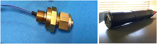
Figure 1. Photo of SST sensor (left) and of MoSens device with HRSST sensor (right).

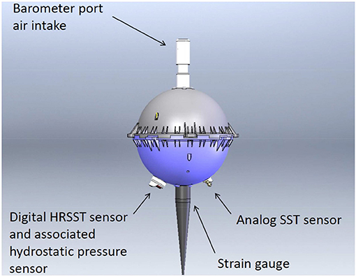
Figure 2. Schema of the buoy with its sensors (the line, the stainless bracket and the holey sock drogue are not represented). Doc. ^® nke Instrumentation.

The HRSST sensor is composed of a thermistor inserted in a small stainless steel needle of 0.9 cm length L and 0.12 cm in diameter D. The resolution is 1 mK and its trueness is expected to be better than 0.01 K.

The HRSST sensor is associated with a hydrostatic pressure sensor in a removable cylindrical housing containing the electronic board of the two sensors. The cylindrical housing is necessary to calibrate these instruments in thermo-regulated baths, but it is removed when these modules are integrated in the buoys. This assembly is called MoSens by nke Instrumentation. The MoSens module hydrostatic pressure sensor presents a theoretical trueness of 0.05% on a range of 0–30 dbar and a resolution of 0.05 dbar. Data are transmitted to the buoy mother-board by a serial link Modbus.

Theoretical Considerations on the Temperature Measurements

de Podesta et al. (2018) demonstrated that “the radiative error for an air temperature sensor, in flowing air depends upon the sensor diameter and air speed, with smaller sensors and higher air speeds yielding values closer to true air temperature.” HRSST and SST analog sensors are protected from direct solar radiations by a cap but one part of the sunlight enters also the ocean. Seawater is close to a blackbody in the infrared part of the spectrum and the blue-green radiations can be reflected at depths as great as 50 m (Le Traon, 2018). In the ocean, light radiations are reflected by particles or phytoplankton, and absorption and scattering decrease strongly their intensity, and hence their effects on exchanged heat flux. This exchange is therefore secondary compared to the impact of convection or conduction. However, one part is backscattered to the surface and can be detected by satellites to measure ocean color. This part can also be detected by sensitive sensors and it is interesting to evaluate the error induced by radiations on the measurement of the true temperature of seawater.

It is therefore interesting to see if de Podesta's affirmation is also true in seawater. He establishes the balance equation between the heat flux exchanged in steady state and the fluxes due to irradiation and self-heating as follows:

where h is the heat transfer coefficient, A = πLD is the surface of exchange of the sensor considered as a cylinder of length L and diameter D, T_S is the temperature of the sensor's surface, T_sw is the true temperature of seawater, I²R is the power of the self-heating due to the current I passing through the sensor resistance R, ϵ_S is the emissivity or absorptivity of the sensor's surface, E is the irradiance, σ is the Stefan-Boltzmann constant, and T_w is the temperature of the walls (surrounding the sensor) assumed to be emitting as a blackbody. The heat transfer coefficient h is the key quantity to understand the intensity of the thermal transfer between the surface of the sensor and the fluid. It takes into account the conjugate effects of conduction, convection, and radiation in the surrounding medium.

We can consider the self-heating as negligible, because the thermistor is fed by a micro-current leading to the maximum error of a few hundred of micro-degrees. If we consider that the radiative environment is almost at the same temperature as the surface of the sensor, T_w ≈ T_S, then the second part of the right-hand-side of Equation (1) can be neglected. The temperature measurement error can then be described by:

For a fluid flowing perpendicularly past a cylinder, h can be approximated by the equation:

where k is the thermal conductivity of the fluid and Nu the Nusselt number for a cylinder in a transverse flow. In the case of water, the following empirical expression is often used to calculate Nu in conditions of laminar flow (Schlichting, 1979):

Pr is the Prandlt number. It describes a fluid with a dynamic viscosity μ and a specific heat capacity C_p:

Re is the Reynolds number. It describes the flow of a fluid which would have a speed V and a density ρ:

The Equation (6) is valid when RePr > 0.2. In the case of a surface seawater with a practical salinity of 35, a temperature of 15°C, even with a very low speed V = 0.001 m s⁻¹, RePr = 8.33 (with D = 1.2 mm). Combining Equations (2–6) gives:

The relation (7) shows that the error due to the irradiance is proportional to the square root of the diameter of the cylindrical sensor (all other parameters assumed equal). Applied to the HRSST sensor with D = 0.12 cm and to the SST analog sensor with an average diameter D = 1.4 cm, the radiative error is divided by 3.4, to the advantage of the HRSST sensor, when the same environmental conditions are considered.

The size difference between the SST analog sensor and the HRSST sensor also has an effect on the response time τ. If we neglect the exchange by radiation, most of the heat exchanged between the sensor and the medium is the result of convection, described by the coefficient h. The quantity of heat propagating in the sensor of mass m and specific heat capacity C_ps, results in a temperature variation dT during the time dt. The balance equation can be written:

Its resolution leads to the equation:

where T₀ is the initial temperature of the sensor and τ is the ratio:

In Equation (9), the time for which t = τ represents the constant 1 – e⁻¹ = 0.632 which defines the response time τ. The Table 1 shows that for a very low seawater velocity and the same environmental conditions, the response time τ is about 7 times larger for the SST analog sensor than for the HRSST sensor. Table 1 also shows the results of (D/V)^0.5 ratios for two flow speeds. Figure 3 shows the response times of both sensors, as a function of velocity.

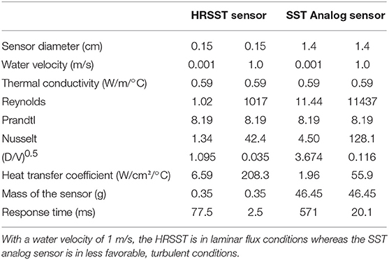
Table 1. Comparison of ratios D/V and response times for the HRSST sensor and the SST analog sensor in a seawater at 15°C and S = 35.

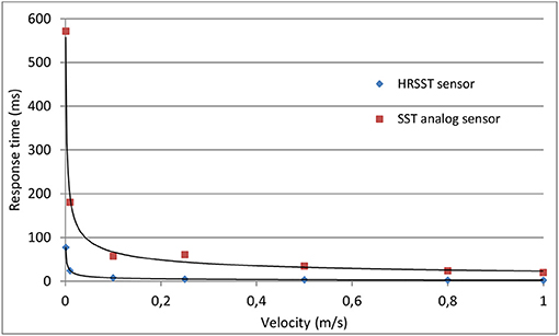
Figure 3. Variation of the sensor response time as a function of the seawater velocity according to relation (8). From at least 0.25 m/s, the SST analog sensor is in turbulent exchange conditions, whereas the HRSST sensor is in laminar conditions even at 1 m/s.

Calibration and Laboratory Tests of the HRSST Sensors

One of difficulties in constituting a 100-buoy reference network is to calibrate all the buoys with an uncertainty close to a few milli-degrees. The solution found was to first calibrate the MoSens devices, then to integrate them in the buoys, and finally to verify the lack of added systematic errors due to the integration. Two prototypes were assembled as proofs of concept.

Calibration and Traceability of Temperature Measurements

The MoSens devices are calibrated by comparison in a calibration bath whose thermal stability shows a standard deviations between 0.1 and 0.3 mK during temperature plateaus. The MoSens sensors are completely immersed and placed close to the sensitive part of an SBE 35 reference thermometer. This thermometer is verified and calibrated periodically in triple point of water (ptH₂O) and fusion point of Gallium (pfGa) cells, to ensure the linkage to the International Temperature Scale of 1990 (ITS-90) of the measured temperatures. The ptH₂O and pfGa cells are calibrated by the French National Institute of Metrology (LNE-CNAM), to 0.1 and 0.26 mK, respectively.

Eight temperature plateaus are created between 1 and 35°C to allow the comparison between the devices and to calculate the coefficients G, H, I, J of the Bennett relation (11), for each MoSens sensor, with a least-squares technique:

where x is the raw value delivered every second by the sensor.

Once the coefficients are obtained and programmed in the MoSens, the calibration verifications are made. For the two prototypes, the residuals of the least squares calculation are between 0 and 1.1 mK, but the verification made in the bath showed that maximum deviations of 2.4 mK could be obtained (see Figure 4), even if most of them are under 2 mK. These deviations can be explained by the thermal inertia and the self-heating of the MoSens modules (see section Measurement of the Response Time of the MoSens Module) equipped with their cylindrical housing. Nonetheless, they remain below the desired threshold values.

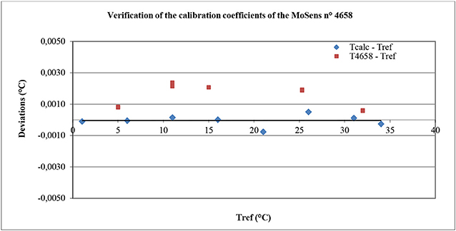
Figure 4. Example of calibration verification made on the MoSens sensor n° 4658. Blue squares represent the residuals and the red squares represent the measured values after the calibration.

Uncertainty of the HRSST Sensors Calibration

The calibration uncertainty budget includes:

– The standard uncertainty on the reference temperatures, u_tref assessed to be 0.9 mK from 0 to 35°C. This includes the calibration of the reference thermometer to the fixed reference points of the ITS-90, its drift over the 12 last months, and its reading uncertainties.

– The uncertainty of the bath stability and homogeneity. According to the standard deviations of the measurement series and to homogeneity measurements made on the bath, the standard uncertainty on the bath stability and homogeneity u_bath can be assessed to be 0.3 mK.

– The reproducibility S and repeatability S_rep of MoSens sensors measurements. The reproducibility is evaluated according to the standard ISO 5725-2 (1994), by calculating the variance of the deviations obtained during the verifications of calibrations. For the prototypes of MoSens n° 4656 and n° 4658, this gives, respectively, S = 1.7 mK and S = 0.9 mK. The repeatability S_rep can be assessed by calculating the average of the standard deviations of the temperatures measured by MoSens sensors. For the two sensors S_rep = 0.3 mK. This repeatability is strongly correlated to the bath stability.

According to this budget, the model used to calculate the combined uncertainty on the deviations D is:

In this equation, T is the average of the series of temperature values given by the sensor under calibration, T_ref is the average reference temperature, δ_rep is the short term variation of the sensor temperature, δ_reprod is the long term variation of the sensor temperature and δ_bath is the difference in temperature due to the stability and the homogeneity of the bath which introduce small errors between T_ref and T at the time of measurements. Applying the GUM method (BIPM, 2008) to relation (12) and assuming a correlation coefficient of 1 between δ_rep and δ_bath yields:

The expanded uncertainty (U_C) on the deviations obtained during the calibration can be calculated by the relation:

Table 2 shows the uncertainty budget and the results of relation (14) for the two buoys. For the n° 4656, U_C = 4.0 mK, and for the n° 4658, U_C = 2.8 mK.

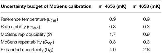
Table 2. Calibration uncertainty budget of the two MoSens prototypes.

Measurement of the Response Time of the MoSens Module

As the MoSens sampling rate is only 1 s, it has been necessary to fix the initial deviation T_sw – T₀ of Equation (9), close to 10°C, to allow the assessment of τ. The τ value has been calculated (see Figure 5) and it gives 0.200 s°C⁻¹ for the n° 4656 instrument and 0.206 s°C⁻¹ for the n° 4658 instrument in nearly static exchange conditions. The time to obtain 99.99% of the final response can be calculated with the relation t_99.99 = τ ln(1 – 0.9999)/1000, and it gives about 1.85 s. The graphical determination of the time to obtain 63.2% of the final response is made with an uncertainty close to 75 ms. It gives a maximum uncertainty value on τ of 17 ms°C⁻¹.

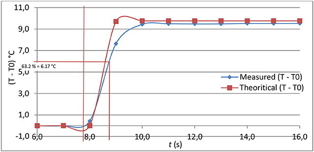
Figure 5. Determination of the response time of MoSens module n° 4656.

The measured values of τ are about 2.5 times the theoretical value given in Table 1 in low flow speed conditions and for the HRSST sensor alone. This can be explained by taking into account the heat exchange of MoSens module, in its PVC housing, with the water by convection and radiation, and with the sensor by conduction. This hypothesis is reinforced by drawing the theoretical response curve of HRSST sensor from the relation (9), in which τ would be equal to 0.2 s (Figure 5). It appears that the slope of the temperature increase is more important that the measured slope. The response of MoSens module cannot be represented by the simple relation (9) and it doesn't represent exactly the response of HRSST sensor.

The PVC housing and the self-heating of the electronic board of MoSens modules have another effect. It takes longer to reach the final temperature to within ±2 mK. The time to obtain T – T₀ = 2 mK is close to 35 min when T_Sw – T₀ is close to 10°C. This time is not representative of the response time at sea because the MoSens devices are integrated in the buoys without their PVC cylindrical housing and it is always at a temperature that is relatively stable or slowly changing. In other words, the operation carried out here to estimate the sensor response time is sub-optimal, and would need repeating with the sensor integrated in the buoy, but this would pose other practical issues.

Verification of the Calibration of HRSST and SST Sensors of Two Buoys

Once calibrated, the two MoSens sensors have been integrated in buoys and these buoys have been placed in the calibration bath. A platinum 100 Ω thermometer has been fixed on one of them and protected from the air temperature variations with a piece of foam (see Figure 6), in order to measure the external temperature of the buoy and to try to detect its influence on the HRSST and SST measurements. In the calibration mode, the buoys acquire data not every second but every 5 s after having taken off the magnet. Even if the bath temperature is very stable, this reduced sampling rate increases slightly the measurement uncertainty.

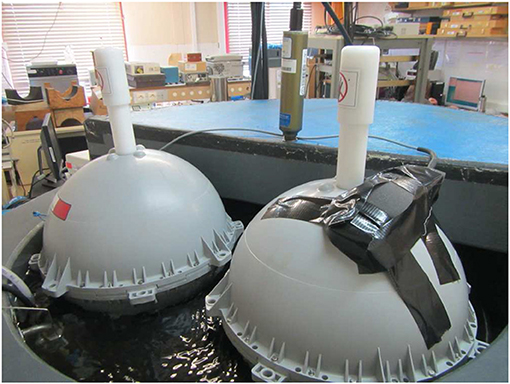
Figure 6. Buoys in the calibration bath, close to the reference thermometer. A pt100 Ω thermometer is fixed on one of them and protected with a piece of foam.

Two verification series have been performed on the two buoys. The first series was from 1 to 34°C, the buoys being in contact with the air in the laboratory. For the second series, from 34 to 1°C, the buoys were covered with a survival blanket. The goal of this second series was to measure the effect, on HRSST and SST analog measurements, of buoy temperatures closer to the water temperature. The blanket has been laid to shield the buoy from radiation within the room and thus to partially insulate the buoy from the room temperature, to enclose the radiations of the bath and to limit the air exchanges.

The results of the first series show that, for the two buoys, the amplitude of the deviations is the same as the amplitudes measured during the verification of MoSens sensors alone (see Figure 7). It means that the integration of MoSens in the buoy does not add systematic errors to the HRSST measurements. Furthermore, this implies that MoSens sensors can be calibrated alone, before integration in the buoys, which is an essential point to develop a fiducial reference network.

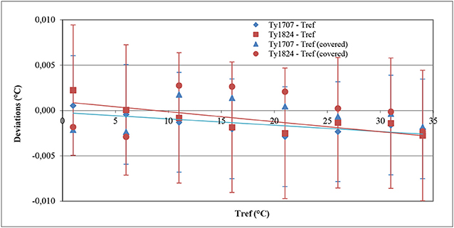
Figure 7. Deviations obtained during the verification of HRSST sensors of two buoys during the two series, with the expanded uncertainty of the verification.

The results of the second series are given in Figure 7 and in Table 3, for the buoy n° Y17-07. The table shows that in spite of buoy temperatures different between the two series (ambient vs. covered) by as much as 3.2°C, the deviations are similar in amplitude to the first series (−0.4 mK at 34°C). It shows also that these deviations are more dependent on the cooling or the warming of the water than of the air temperature, because the maximal deviation is obtained at 16°C and at this temperature, the difference in external buoy temperatures is only 0.7°C. Figure 7 shows that:

– At 35°C the points are superimposed because it is the last point of the first series and the first point of the second series.

– From 27 to 12°C the deviations show the buoy temperatures are higher than the reference temperatures, probably because of the thermal inertia of the ensemble MoSens-Buoy, as the temperatures of the bath is gradually reduced.

– At 1 and 6°C, the deviation is inversed because the temperature has been generated in increasing order.

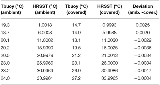
Table 3. Differences between buoys and HRSST ambient and covered temperatures for the buoy n° Y17-07.

The two measurement series realized on the two buoys can be used to assess in details the reproducibility of temperature measurements. By using the deviation (amb.—cover.) (see Table 3 for n° Y17-07), the relation (14) gives another estimation of the expanded measurement uncertainty of two buoys. Table 4 shows the results. The main source of uncertainty comes from the reproducibility of measurements impacted by the thermal inertia of buoys. Expanded uncertainties are expressed with a coverage factor of 2 including 95.5% of measurements in the case of Gaussian distributions. They are inferior to 0.01°C.

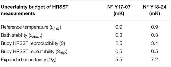
Table 4. Uncertainty budget of buoys HRSST measurements.

During the two series of HRSST calibration, the temperatures of the SST analog sensors have also been recorded. They have been calibrated by the manufacturer in the range 5–35°C. Figure 8 shows the results of the verification. The deviations are inferior to ±0.1°C, even for the point at 2°C, which is outside the calibration range. If we exclude this point, it is possible to improve the trueness and the uncertainty of SST measurements by calculating the coefficients of a straight line. By considering this linear correction, it is possible to assess the measurement uncertainties of these two SST analog sensors by using the same procedure as for the HRSST sensors. However, it is necessary to take into account a residual linearity error. The results are given in Table 5. The expanded uncertainty of SST analog sensors is found to be twice as large as the expanded uncertainty of HRSST sensors. One must keep in mind in addition that the SST analog sensor is much slower to respond than the HRSST sensor, and that it is also more sensitive to radiation effects. All these effects contribute to additional larger systematic errors or measurement uncertainties.

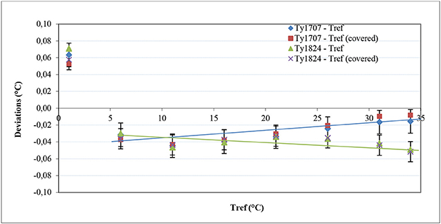
Figure 8. Deviations obtained during the verification of SST sensors of two buoys during the two series, with the expanded uncertainty of the verification.

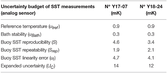
Table 5. Uncertainty budget of buoys SST measurements in the range 6–35°C.

Utility and Laboratory Test of the Hydrostatic Pressure Sensor

In order to try to reduce the uncertainty in the HRSST measurement depth, the MoSens have been equipped with a hydrostatic pressure sensor located near the HRSST sensor. The immersion depth d of the water pressure sensor is given by the buoy geometry, d = R cos(α) where R is the radius of the spherical buoy and α is the angle of placement of the sensor in the spherical buoy (measured from the vertical), but this distance from the waterline can vary with the seawater density ρ_w and the traction made by the drogue, but also with the variations of α during rough sea conditions.

During calm sea conditions, the air pressure sensor measuring p_a is at the level of the waterline. Therefore, d can be obtained from the measurement of the pressure p:

where g is the acceleration of gravity at the buoy location (this value depends on latitude in first approximation, for a body that remains on the ocean surface). In this relation, ρ_w needs an assessment of the salinity to be determined with a sufficient accuracy.

When the buoy is in rough sea conditions, or oscillating (rotating) around its center of gravity, it is submitted also to a vertical acceleration a_g added to g. If a_g values are close to g the measurements of water pressure cannot be used directly to retrieve depth without ad hoc processing and filtering, but the time-series of pressure at high-frequency can provide an indication of the sea state. This information can be of use to determine whether the water is well-stratified or well-mixed, assuming that the air pressure is stationary (this hypothesis does not hold if the buoy is oscillating up and down in waves with heights of several meters). For comparison with satellite measurements, a well-mixed top layer may suggest that emission from the surface is at the measured water temperature, whereas a stratified top layer may suggest that the radiated temperature may need to be corrected (based on wind and radiation conditions).

Results shown by Poli et al. (2016) corroborate these assertions. When two temperatures measured by previous HRSST buoys are compared, the differences can be reduced to within the digital sensor trueness by considering only well-mixed conditions, selected when the waves in the ERA-Interim (Dee et al., 2011) reanalysis are above 3 m in significant wave height. Another application of trying to infer the sea-state is to better parameterize the emissivity to be used for simulating the radiances seen by the satellite, especially for microwave instruments, with rough seas or swell suggesting white caps and foam (Niclòs et al., 2007).

During the temperature verifications of the two buoys, the MoSens pressure sensors data have been recorded to observe their drift with respect to temperature. A reference atmospheric pressure P_atm has been measured with a recently calibrated WIKA CPC 8000 pressure calibrator. It was therefore possible to calculate a reference pressure P_ref = d + (P_atm – 1013.25)/100, to observe the pressure drifts of sensors as a function of the temperature.

The immersion depth d was estimated to be 0.13 m in the bath (without the weight of the drogue, which remained outside the calibration bath). The results show that the external temperature of the buoy has no significant effect on the measured pressures, but that the temperature of the water leads to maximum systematic errors of ±0.15 dbar between 0 and 35°C. They also show that this effect is linear and that this technology of sensor reacts with a good reproducibility to temperature variations. This behavior can hence be corrected for each buoy: a straight line correction curve yields residual errors inferior to ±0.004 dbar (or 4 mm of water). Since the slopes and offsets for the two sensors are very similar, it is possible to consider correcting the two instruments with average coefficients. The residual errors obtained with the average coefficients slope = −0.0077 dbar/°C and offset = 1.499 dbar are inferior to ±0.02 dbar, which is close to the accuracy claimed by the manufacturer, and in relation with the technology of the sensors. The same coefficients may be applied to future buoys.

Trials at Sea and Comparison With a CTD Profiler

While the initial concept of buoy development using a pre-calibrated sensor was demonstrated to work in the laboratory, two further elements are needed to build a FRM drifter network. The first element is to demonstrate that the trueness estimate still holds, once the buoys are deployed in the target environment (at sea). The second element is to demonstrate that the trueness estimate remains valid for the lifetime of the buoy (i.e., no significant temporal drift). While it is too early to study the second element, this section explores the first one.

The two prototype buoys were deployed at sea during an oceanographic cruise in Mediterranean Sea. After unpacking on the ship deck to test the transmission and the good transmission of the Iridium SBD messages, a comparison with a CTD profiler (SBE 911⁺) was set up. The CTD profiler was fixed under a Multi-Bottle Sampling Array (MBSA), with a reference thermometer SBE 35 calibrated in the fixed point cells of the ITS-90. The drifters were held in place near the ship by means of a line. When the MBSA was completely immersed, the CTD and the SBE 35 temperature measurements were recorded at about 1 m under the surface. After the surface measurements were collected, the MBSA was lowered to 15 m depth in order to estimate the temperature profile of the first layers. This profile showed that in the four first meters, the temperature of the water was homogeneous and close to 16.4°C, allowing fair comparison with the HRSST buoy. Between 4 and 5.5 m (the depth where Argo floats surface temperature measurements are sometimes used as reference) there was a strong temperature gradient of −1.25°C m⁻¹. Until 15 m depth, the temperature was still very stable but shifted by about 2°C as compared to the surface.

During the subsurface waiting time, 5 measurement series of 29, 57, 113, 53, and 149 values were made with the SBE 35 sampling at 1 Hz, giving an average temperature of 16.3968°C with a standard deviation of 0.0057°C. The CTD temperature at 1.08 m depth is very close to this value: 16.398°C. Table 6 gives the results of the comparison with the values transmitted by the buoys. The first two lines show the results for the SST analog sensors and the following for the HRSST sensors. In the second column of this array, SST temperatures from the analog sensors have been corrected with the slopes and offsets coefficients of the straight lines of Figure 8, in order to fairly compare with what may be expected, at best, from low-cost SST sensors with ideal calibration.

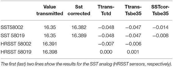
Table 6. Results of the comparison made at sea, between buoys transmitted values, CTD and SBE 35 measurements.

The results of this comparison show that without any correction, HRSST values are in the standard dispersion range of the SBE 35 and the deviations compared to CTD and SBE 35 are inferior to 0.01°C. Without corrections, SST deviations from analog sensors are close to −0.05°C and with the corrections calculated in the metrology laboratory, they are within the calculated expanded uncertainties of buoys SST sensors, and also within the estimated standard deviations from the percentiles transmitted by the buoys.

This comparison at sea shows firstly that the temperature values transmitted by the buoys are not erroneous. Secondly, regarding the HRSST sensors, the deviations obtained in comparison to two independent instruments, are small and probably representative of the dispersion of the medium temperatures. They are inferior to the deviations obtained with the SST analog sensors, even after linear correction of SST transmitted values, probably because of their better response time, resolution and calibration uncertainties.

After this comparison, buoys were released in an eddy feature. The details of this deployment are given by Poli et al. (2018). After initial deployment on 26th April 2018, the buoys were initially separated by <1 km and they remained within 10 km of each other until 23rd May. After that, they quickly diverged until the first one ran ashore. At the time of initial writing of this paper, the second buoy was still drifting with its drogue, five and a half month after its deployment.

According to Poli et al. (2018), this comparison showed that “once freely drifting, the buoys observe that the SST spread within 5 min is usually smaller than 0.1 K, especially when the sea-state is well-mixed and the buoys are within an eddy core. The availability of percentiles from the 5-min distribution of SST sampled at 1 Hz (by a sensor with a fast response time) should help users improve their data processing chain to move toward an ensemble approach.” The results of this other paper suggest also that “it is important to consider the sea-state mixing and the ocean surface circulation to understand the representativeness of the in-situ SST data, as they both affect observed SST variations (within the day and within 5 min). Consequently, they may both be worth taking into account in the process of satellite SST cal/val.”

Conclusion

The goal of this study relates to the conception and the metrological characterization of new surface drifting buoys, design to comply with the requirements of SST satellites measurements validation and to link through comparison these measurements to the SI. This linkage can be achieved by the calibration of each buoy and the assessment of the instrumental measurement uncertainty, taking into account all the elements of the temperature calibration chain.

Calibrating individually 100 drifting buoys in a calibration bath is time-consuming and unrealistic. This study shows that it is possible to calibrate the sensors and their conditioning electronic circuits beforehand, without adding significant errors or uncertainties to in situ measurements even once the sensors have been integrated in buoys, and to keep the instrumental uncertainty under the tolerance of 0.01°C. This was possible through the design of the MoSens modules which include high resolution temperature sensors and hydrostatic pressure sensors. The concept of high resolution includes the possibility to make temperature measurements with a repeatability close to a milli-degree, a fast thermal response time measured in laboratory and a fast sample rate (1 Hz).

The measurements made on the two buoys have also enabled the improvement of the calibration of the SST analog sensors. If, initially, their measurement errors are already included in the ±0.1°C tolerance, it is possible, by using slope and offset correction coefficients, to obtain instrumental expanded measurements uncertainties inferior to 15 mK. With these corrections, in situ comparisons have shown that it is possible to reduce the deviation of 0.047 to −0.014°C for one sensor and −0.008°C for the other. However, this correction procedure requires each buoy to be placed in the calibration bath. This is not feasible for an industrial process to ensure repeated accuracy. Also, one must bear in mind that the large size of the SST analog sensors makes them much slower to respond to seawater variations than smaller HRSST sensors, as shown in this paper.

The temperature-dependence of the MoSens pressure sensor has also been studied. It can lead to errors of ±0.15 dbar in the temperature range 0–35°C. These errors can be compensated with average slope and offset coefficients to improve the determination of HRSST measurements depth during calm sea conditions. In rough sea conditions, this sensor provides an indication of the sea-state, which is essential to understand the deviations between satellites and buoys temperature measurements. The relationship between information contained in the high-frequency data and the sea state should be explored in future work.

The specifications of two prototypes measured in laboratory, have been confirmed during the initial deployment at sea by a comparison to a reference thermometer SBE 35 and a CTD profiler, demonstrating also the good transmission of data and the very good trueness of HRSST measurements in a homogeneous medium.

Future prospects include deploying at least 100 SVP-BRST units, with the aim of closing the metrological loop with buoys that would be recovered from sea, to be verified in a calibration bath. An experiment will also be carried out with a SVP-BRST buoy kept over a long duration at a fixed position at sea, next to a reference moored buoy. This will allow to determine whether or not the SVP-BRST buoys remain within the initial tolerance of 0.01°C.

Author Contributions

MLe: responsible for the metrology part. PP: concept of measurements, deployment of buoys, and data processing. AD and JS: buoy developer. MLu: responsible of the project and data processing. AO'C: initiator of the project and the requirements. MB: metadata transmission and processing. KH: trials at sea.

Funding

This work was a part of the TRUSTED project led by Collecte Localisation Satellite (CLS) following a call to tender by EUMETSAT. TRUSTED is a Copernicus project, funded by the European Commission.

Conflict of Interest Statement

AD and JS were employed by company nke Instrumentation.

The remaining authors declare that the research was conducted in the absence of any commercial or financial relationships that could be construed as a potential conflict of interest.

References

Banks, A. C., Mittaz, J., Bialek, A., Woolliams, E., Nightingale, J., Fox, N., et al. (2017). “Metrology in satellite oceanography,” in Conference: Second National Physical Laboratory (UK) – National Institute of Metrology (China) Joint Symposium (Teddington: NPL).
BIPM (2008). Evaluation of Measurement Data – Guide to the Expression of Uncertainty in Measurement. JCGM 100:2008.
BIPM (2012). International Vocabulary of Metrology – Basic and General concepts and Associated Terms (VIM), 3rd Edn. JCGM 200.
Blouch, P., Billon, C., and Poli, P. (2018). Recommended Iridium SBD Dataformats for Buoys (Version 1.7). Zenodo.
Castro, S. L., Gary, A. W, and William, J. E. (2012). Evaluation of the relative performance of sea surface temperature measurements from different types of drifting and moored buoys using satellite-derived reference products. JGR Oceans 117:C2. doi: 10.1029/2011JC007472
de Podesta, M., Bell, S., and Underwood, R. (2018). Air temperature sensors: dependence of radiative errors on sensor diameter in precision metrology and meteorology. Metrologia 55, 229–244. doi: 10.1088/1681-7575/aaaa52
Dee, D. P., Uppala, S. M., Simmons, A. J., Berrisford, P., Poli, P., Kobayashi, S., et al. (2011). The ERA-Interim reanalysis: configuration and performance of the data assimilation system. Q. J. R. Meteorol. Soc. 137, 553–597. doi: 10.1002/qj.828
Donlon, C., Berruti, B., Buongiorno, A., Ferreira, M.-H., Femenias, P., Frerick, J., Sciarra, R., et al. (2012). The Global Monitoring for Environment and Security (GMES) Sentinel-3 mission. Remote Sens. Env. 120, 37–57. doi: 10.1016/j.rse.2011.07.024
Donlon, C. J., Nykjaer, L., and Gentemann, C. (2004). Using sea surface temperature measurements from microwave and infrared satellite measurements. Int. J. Remote Sens. 25, 1331–1336. doi: 10.1080/01431160310001592256
EGOS (2002). Minimum Specifications and Guidelines for the Operation of EGOS Drifting Buoys. Technical Document.
Gaillard, F., Diverres, D., Jacquin, S., Gouriou, Y., Grelet, J., Le Menn, M., et al. (2015). Sea Surface Temperature and Salinity from French research Vessels, 2001-2013. Nat. Sci. Data 2:150054. doi: 10.1038/sdata.2015.54
Hausfather, Z., Cowtan, K., Clarke, D. C., Jacobs, P., Richardson, M., and Rohde, R. (2017). Assessing recent warming using instrumentally homogeneous sea surface temperature records. Sci. Adv. 3:e1601207. doi: 10.1126/sciadv.1601207
Immler, J. F., Dykema, J., Gardiner, T., Whiteman, D. N., Thorne, P. W., and Vomel, H. (2010). Reference quality upper-air measurements: guidance for developing GRUAN data products. Atmos. Meas. Tech. 3, 1217–1231. doi: 10.5194/amt-3-1217-2010
ISO 5725-2 (1994). Accuracy (Trueness and Precision) of Measurement Methods and Results - Part 2: Basic Method for the Determination of Repeatability and Reproducibility of a Standard Measurement Method. Available online at: https://www.iso.org/
Kennedy, J. J. (2014). A review of uncertainty in in situ measurements and data sets of sea surface temperature. Rev. Geophys. 52, 1–32. doi: 10.1002/2013RG000434
Kennedy, J. J., Rayner, N. A., Smith, R. O., Saunby, M., and Parker, D. E. (2011a). Reassessing biases and other uncertainties in sea-surface temperature observations since 1850 Part 1: measurement and sampling errors. J. Geophys. Res. 116:D14103. doi: 10.1029/2010JD015218
Kennedy, J. J., Smith, R., and Rayner, N. (2011b). Using AATSR data to assess the quality of in situ sea surface temperature observations for climate studies. Remote Sens. Environ. 116, 79–92. doi: 10.1016/j.rse.2010.11.021
Kent, E., and Berry, D. (2008). Assessment of the Marine Observing System (ASMOS): Final Report. Technical Report. National Oceanography Centre, Southampton.
Le Traon, P. Y. (2018). “Satellites and operational oceanography,” in New Frontiers in Operational Oceanography,” eds E. Chassinet, A. Pascual, J. Tintoré, and J. Verron (GODAE Ocean View), 161–190. doi: 10.17125/gov2018.ch07
Lewellyn-Jones, D., Edwards, M. C., Mutlow, C. T., Birks, A. R., Barton, I. J., and Tait, H. (2001). AATSR: global-change and surface-temperature measurements from ENVISAT. ESA Bull. 105, 10–21.
Lumpkin, R., and Pazos, M. (2006). “Chapter 2: Measuring surface currents with Surface Velocity Program drifters: the instrument, its data, and some recent results,” in Lagrangian Analysis and Prediction of Coastal and Ocean Dynamics (LAPCOD), eds A. Griffa, A. D. Kirwan, A. J. Mariano, T. Ozgokmen, and T. Rossby (Cambridge: Cambridge University Press, 39–67. doi: 10.1017/CBO9780511535901.003
Merchant, C. J., Embury, O., Rayner, N. A., David, I. B, Corlett, G. K., Lean, K., et al. (2012). A 20 year independent record of sea surface temperature for climate from Along-Track Scanning Radiometers. J. Geophys. Res. 117:C12013. doi: 10.1029/2012JC008400
Merchant, C. J., Holl, G., Mittaz, J., and Woolliams, E.R. (2019). Radiance uncertainty characterisation to facilitate climate data record creation. Remote Sens. 11:474. doi: 10.3390/rs11050474
Milman, A. S., and Wilheit, T. T. (1985). Sea surface temperatures from the scanning multichannel microwave radiometer on Nimbus 7. J. Geophys. Res. 90, 11631–11641. doi: 10.1029/JC090iC06p11631
Niclòs, R., Caselles, V., Valor, E., and Coll, C. (2007). Foam effect on the sea surface emissivity in the 8–14 mm region. J. Geophys. Res. 112:C12020. doi: 10.1029/2007JC004521
O'Carroll, A., Eyre, J. E., and Saunders, R. W. (2008). Three-way error analysis between AATSR, AMSR-E, and in situ sea surface temperature observations. J. Atmos. Ocean. Technol. 25, 1197–1207. doi: 10.1175/2007JTECHO542.1
Oka, E. (2005). Long-term sensor drift found in recovered argo profiling floats. J Ocean. 61, 775–781. doi: 10.1007/s10872-005-0083-6
Poli, P., Emzivat, G., Blouch, P., Férézou, R., and Cariou, A. (2016). “Météo-France/E-SURFMAR HRSST (re)calibration,” in GHRSST Workshop on Traceability of Drifter SST Measurements (La Jolla, CA: Scripps Institution for Oceanography).
Poli, P., Lucas, M., O'Carroll, A., Le Menn, M., David, A., Corlett, G. K., et al. (2018). The Copernicus Surface Velocity Platform drifter with Barometer and Reference Sensor for Temperature (SVP-BRST): genesis, design, and initial results. Ocean Sci. 15, 199–214. doi: 10.5194/os-2018-109
Prabhakara, C., Dalu, G., and Kunde, V. G. (1974). Estimation of sea surface temperature from remote sensing in the 11- to 13-μm window region. J. Geophys. Res. 79, 5039–5044. doi: 10.1029/JC079i033p05039
Roemmich, D., and Gilson, J. (2009). The 2004-2008 mean and annual cycle of temperature, salinity and steric height in the global ocean from the Argo program. Prog. Oceanogr. 82, 81–100. doi: 10.1016/j.pocean.2009.03.004
Sybrandy, A. L., Niiler, P. P., Martin, C., Scuba, W., Charpentier, E., and Meldrum, D. T. (2009). Global Drifter Programme Barometer Drifter Design Reference. DBCP Technical Report, Published by the Data Buoy Cooperation Panel (DBCP), Geneva, Switzerland.
Titchner, H. A., and Rayner, N. A. (2014). The Met Office Hadley centre sea ice and sea surface temperature data set, version 2: 1. sea ice concentrations. J. Geophys. Res. Atmos. 119, 2864–2889. doi: 10.1002/2013JD020316
Woolliams, E. R., Mittaz, J., Merchant, C. J., Dilo, A., and Fox, N. P. (2016). “Uncertainty and correlation in level 1 and level 2 products: a metrologist's view,” in Living Planet Symposium, Proceedings of the Conference, ed L. Ouwehand (Prague), 80.
Woolliams, E. R., Mittaz, J., Merchant, C. J., Hunt, S. E., and Harris, P. M. (2018). Applying metrological techniques to satellite fundamental climate data records. J. Phys. Conf. 972:012003. doi: 10.1088/1742-6596/972/1/012003
Keywords: drifting buoys, surface temperature, reference, satellite, measurement uncertainty, SST
Citation: Le Menn M, Poli P, David A, Sagot J, Lucas M, O'Carroll A, Belbeoch M and Herklotz K (2019) Development of Surface Drifting Buoys for Fiducial Reference Measurements of Sea-Surface Temperature. Front. Mar. Sci. 6:578. doi: 10.3389/fmars.2019.00578
Received: 08 January 2019; Accepted: 30 August 2019;
Published: 13 September 2019.
Edited by:
Leonard Pace, Schmidt Ocean Institute, United StatesReviewed by:
Shinya Kouketsu, Japan Agency for Marine-Earth Science and Technology, JapanR. Venkatesan, National Institute of Ocean Technology, India
Copyright © 2019 Le Menn, Poli, David, Sagot, Lucas, O'Carroll, Belbeoch and Herklotz. This is an open-access article distributed under the terms of the Creative Commons Attribution License (CC BY). The use, distribution or reproduction in other forums is permitted, provided the original author(s) and the copyright owner(s) are credited and that the original publication in this journal is cited, in accordance with accepted academic practice. No use, distribution or reproduction is permitted which does not comply with these terms.
*Correspondence: Marc Le Menn, Marc.lemenn@shom.fr