The potential of flood forecasting using a variable-resolution global Digital Terrain Model and flood extents from Synthetic Aperture Radar images

Introduction

Globally, flooding accounts for a substantial proportion of the fatalities and economic losses caused by natural hazards. In Europe alone, there were 100 major floods between 1998 and 2011, causing more than 700 deaths, the displacement of over 500,000 people and 25 billion euro of insured losses. In the UK, the devastating floods of summer 2007 cost a total of £3.2 billion, and caused the country's worst peacetime emergency since WW2. The impact of climate change means that the probability of events of a similar scale happening in the future is increasing (Allan and Soden, 2008).

Flood inundation models are commonly used to model river flooding. A basic data requirement of these models is a Digital Terrain Model (DTM) of the river reach being studied. The scale at which modeling is required determines the accuracy required of the DTM. For modeling floods in urban areas, a high resolution DTM such as that produced by airborne LiDAR (Light Detection And Ranging, ~1 m spatial resolution, 0.2 m height accuracy) or airborne InSAR (Interferometric Synthetic Aperture Radar, ~5 m spatial resolution, ~1 m height accuracy) is most useful. Many developed countries in the world, including those in Europe, the USA and Australia have now mapped substantial parts of their terrain, including the main river catchments, using LiDAR. A global low-cost DTM containing all the high resolution DTM data currently acquired (and to which more were added as they became available) would be a useful tool for hydrologic and hydraulic modelers, as suggested by Schumann et al. (2014). For example, a modeler in the UK wanting to model urban flooding in Australia would be able to access the necessary DTM data directly, while at present accessing such data might be a severe impediment to modeling. There are obviously substantial logistical and implementational difficulties in creating such a global high resolution DTM, for example concerning ownership of data, intellectual property rights and the creation of a common data format, but, if these could be overcome, the impact of such a DTM would be significant.

In more remote parts of the world a high resolution DTM would contain no data. However, in these areas it is still possible to model flooding on a larger scale using lower resolution DTMs. Since 2000, the Shuttle Radar Topography Mission (SRTM) Digital Elevation Model (DEM) has been used in a number of studies of large-scale river modeling (see Yan et al., 2015). However, in the near future the global DTM of choice is likely to be that derived from the TanDEM-X DEM produced (like the SRTM DEM) using satellite interferometry. This will have a spatial resolution of 10–12 m, and a relative height accuracy of less than 2 m on slopes less than 20% and 4 m on slopes greater than 40% (Eineder et al., 2012). A variable-resolution global DEM obtained by combining existing high and low resolution data sets would be useful for modeling flood water dynamics globally, at high resolution wherever possible (e.g., in urban areas in developed countries) and at lower resolution over larger rivers in remote areas. For example, with the advent of very high resolution global flood modeling for risk management and forecasting, such a DTM would be of great use to help improve predictions and decision making (e.g., Pappenberger et al., 2012; Beven et al., 2015; Bierkens et al., 2015).

A further important data resource used in flood modeling is the extent of the flood over time. High resolution satellite SAR sensors are commonly used to acquire flood extents because they allow images to be taken from space over a wide area, can see through clouds, and can acquire images at night-time as well as during the day. Flood extents derived from SAR imagery may be used for damage assessment and flood defense design studies, and, if obtained in near real-time, for flood relief management and improved flood forecasting (Mason et al., 2014).

Flood extents become more useful if they are intersected with the DTM of the floodplain (e.g., Raclot, 2006; Matgen et al., 2010; Schumann et al., 2011; Garcia-Pintado et al., 2013). Water level observations (WLOs) at the flood boundary can then be estimated at various points along a river reach, and these can be assimilated into a flood inundation model to keep the model “on track” and improve the flood forecast. When used in hindcast mode, they can be used to obtain better estimates of dynamic footprints of past flood events. Fundamental to this approach are the spatial resolution and height accuracy of the underlying DTM. A global DTM used in conjunction with SAR-derived flood extents would allow WLOs to be estimated remotely for any flood in the world, at a level of accuracy determined by the resolution and accuracy of the DTM at that location.

To illustrate the utility of such a DTM, two examples of recent research involving WLOs at opposite ends of the spatial scale are discussed. The first requires high resolution spatial data, and uses a real sequence of high spatial and temporal resolution SAR images (possibly the best example of the sequential monitoring of flood extent by high resolution SAR currently available). WLOs from this are assimilated into a flood inundation model of a river network, in order to update the model state with observations over time, and to simultaneously estimate river discharge and model parameters, including river bathymetry and friction. For many of the world's rivers, their discharges, river depths (bathymetry) and resistance to water flow (friction) are either unknown or poorly known. The sequence of WLOs is used to constrain the uncertainties in this joint estimation problem.

The second example is at a larger scale, and uses the SAR-derived water level observations to improve a lower-resolution DTM such as that derived from the TanDEM-X DEM in the area covered by the flood extents. This improvement to the DTM can be significant and would be permanent, and could be carried out in addition to using WLOs for assimilation to improve a large-scale flood model.

High Resolution SAR-supported Flood Forecast in River Networks

Introduction

The first example considers the sequential assimilation of SAR-derived WLOs of the floodplain into a hydraulic model to decrease forecast uncertainty, using a sequence of real SAR images in a case study. Full details are given in Garcia-Pintado et al. (2015), and what follows in this section is a summary.

The computer models used for flood forecasting solve the mathematical equations governing the flow of water over the local terrain and predict the water levels as a function of time during the flood. Flood inundation is difficult to model due to the complexity of the mathematical equations describing the flow, and to uncertainties in the input flow rates, the bottom friction parameters and the river bathymetry. These uncertainties can be partly compensated for by updating the model state with observed information as this becomes available, to help keep the model on track. The process of updating the model state with observations is known as data assimilation. This takes into account the uncertainties in the observations and model prediction and provides a more accurate estimate of the current state of the system. As well as correcting the model state, assimilation can also improve the estimates of the input flow rates, bottom friction parameters and river bathymetry.

Previous studies using SAR-derived WLOs for river flood monitoring and forecasting have tended to focus on specific single river transects, albeit sometimes ones that are very large or subject to secondary lateral inflows (e.g., Roux and Dartus, 2008; Matgen et al., 2010; Durand et al., 2014). This study used real SAR data for the sequential monitoring and forecasting of a flood developing on a river network which included tributaries. It had two main objectives:

(a) To investigate whether assimilation was best performed using a local or a global filter. The filter used was an Ensemble Kalman Filter (EnKF) (Evensen, 1994), which is a limited-size ensemble representation of the forecast error covariance matrix that is updated as each set of observations is assimilated. The global ensemble error covariances tend to underestimate the forecast error variance and develop physically unrealistic or spurious correlations. This may lead to ensemble collapse and filter divergence. Filter localization is often used to reduce the problem of spurious correlations. This increases the degrees of freedom available to fit nearby observations in the analysis by decreasing the weight given to observations far from the physical location of the estimated state variable (Hamill et al., 2001; Petrie and Dance, 2010).

(b) To investigate whether it was better to focus simply on model state estimation of the water levels, or to simultaneously attempt model state and model parameter estimation.

Methods

Study Area and Models Employed

The study was based on a real event that occurred on the Lower Severn and Avon rivers in the south-west UK in November 2012. Figure 1 depicts the study area for the flood inundation model, covering a 30.6 × 49.8 km² domain.

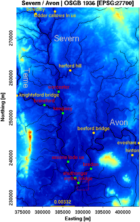
Figure 1. Study domain. OSGB 1936 British National Grid projection, coordinates in meters. Gray labels indicate the three larger rivers (thick black lines). The red polygon surrounds the Tewkesbury urban area. Orange labels/dots refer to the 7 inflow boundary conditions, some of them on smaller tributaries (thin black lines). The yellow line to the South indicates a free-surface boundary condition, with the label indicating the mean bed slope. Red labels/green dots show locations with available stage observations, just used for validation in the forecast model. The background is the ~75 m resolution DEM used for the model, obtained by upscaling the ~5 m NEXTMAP British digital terrain model (after Garcia-Pintado et al., 2015).

In the experimental setup, a real forecast scenario was simulated in which precipitation data was observed rather than forecast, using a network of tipping-bucket gauges sparsely distributed over a 190 W-E × 120 km S-N rectangular area covering seven catchments discharging into the flood domain. With precipitation and potential evapotranspiration as input data, and flow at the outlet of each catchment (yellow names in Figure 1) as calibration data, a single lumped catchment-scale rainfall-runoff hydrologic model (HSPF, Donigian et al., 1995) was calibrated for each catchment using a previous flood event from July 2007. The calibrated discharge of the hydrologic models was used as input to the flood inundation model, to calibrate the latter using time series of water levels at a number of gauges (green points in Figure 1) as calibration data.

The flood inundation model used was LISFLOOD-FP, a coupled 1D/2D model based on a raster grid (Bates and De Roo, 2000). This was applied in the sub-grid formulation of Neal et al. (2012), which utilizes gridded river network data and assumes a rectangular channel geometry. A 75 m resolution grid was employed. After each assimilation step, the model was re-initialized with the updated state vector (i.e., water level).

Using the calibrated hydrologic/flood inundation models, assimilation was conducted with a number of filter configurations for the November 2012 event in a hindcasting scenario.

SAR Image Processing

Satellite SAR observations of the event were acquired by the COSMO-SKyMed (CSK) constellation. A sequence of 7 CSK Stripmap images giving good synoptic views of the flooding was acquired on roughly a daily basis covering the period 27 November—4 December 2012 (Figure 2). The first image in the sequence was acquired just before the flood peak in the Severn (see Figure 3).

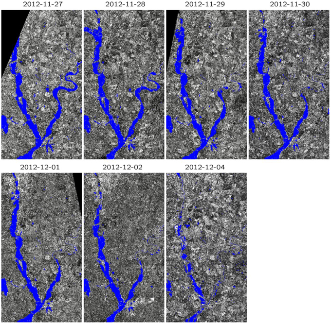
Figure 2. Flood extents (blue) for the event of November 2012, overlain on SAR imagery of the flooded domain of Figure 1 (©CSK) (after Garcia-Pintado et al., 2015).

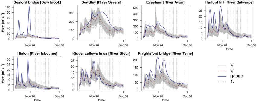
Figure 3. Inflows into the flood domain for the event of November 2012. Blue lines (gauge) are inflows as measured by standard gauges (not used as data input here). Gray lines are the 150-member forecast ensemble (Ψ) from the hydrologic models, used as input by the flood model. Dashed red lines are the ensemble means ($\overline{\Psi }$). Vertical dashed lines show COSMO-SkyMed overpass times (t_y) (after Garcia-Pintado et al., 2015).

In the absence of significant surface water turbulence due to wind, rain or currents, flood water generally appears dark in a SAR image because the water acts as a specular reflector, reflecting backscatter away from the satellite. Detection of the flood extent in each image was performed using the segmentation technique described in Mason et al. (2012a), which groups the very large numbers of pixels in the scene into homogeneous regions. A critical step is the automatic determination of a threshold on the region mean SAR backscatter, such that regions having mean backscatter below the threshold are classified as flooded, and others as un-flooded. The accuracy of the flood inundation maps in rural areas using the algorithm has been determined to be about 90% (Mason et al., 2012a). Figure 2 shows the flood extents detected in the images overlain on the SAR data in the flood inundation model domain. The sequence shows the flood wave moving down the river, and the flood at Tewkesbury gradually dying away, starting on the Avon.

Water level observations (WLOs) were extracted from the flood extent waterlines by intersecting the extents with high resolution floodplain topography from airborne LiDAR using the method described in Mason et al. (2012b). The method selects candidate waterline points in flooded rural areas having low slope and vegetation, so that small errors in waterline position have little effect on waterline level. The standard deviation of the selected WLOs was estimated to be 0.25 m.

Bathymetry Estimation

Field surveyed river cross-sections were available along the Avon and part of the Severn from its junction with the Avon to ~10 km upstream. These were transformed into rectangular equivalents as required by the flood model. Then, for both the Severn and Avon, river widths and depths were interpolated along the river chainage. For the other rivers in the network, as their widths were known, depths were calculated from the widths using a power law relationship (see Garcia-Pintado et al., 2013). The resulting bathymetry was treated as an uncertain parameter in the assimilation procedure. This reflected the fact that detailed river bathymetry is unknown for many of the world's rivers.

The Ensemble Filter

Assimilation was conducted at the time of the corresponding CSK overpasses, so that the flood model simulations were sequentially interrupted. Uncertain friction, bathymetry and errors in inflow boundary conditions were simultaneously estimated at the time of the assimilation by using state space augmentation, in which the model state vector is augmented with these model parameters (Friedland, 1969). An advantage of this approach is that the assimilation scheme is able to take into account correlations between the errors in the parameters and the errors in the model variables (Smith et al., 2013).

The Ensemble Kalman Filter (EnKF) is characterized by a two-step feedback loop i.e., a prediction followed by an observation-based state update. In the prediction phase, each individual ensemble member is evolved forward in time by the forecast model until the time of the next observation. This means that the model states (water-levels) are forecast by the hydrodynamic model with appropriate forecast boundary conditions. At the time of an observation, an ensemble approximation of the Kalman filter equations is used to update the ensemble. This update may be thought of as a linear combination of the forecast and the observations, weighted by the relative uncertainties in the model and observation data. The weights involved are contained within the Kalman gain matrix K (see Garcia-Pintado et al., 2015). An ensemble size of 150 samples was used. An outlier analysis was employed to remove any unlikely observations not accounted for in the model dynamics.

Filter Localization

Typically the number of ensemble members is much smaller than the dimension of the state vector, leading to under-sampling. This often manifests itself as spurious (unphysical) forecast error correlations, which contribute to significant increments updating the state at locations further from the location of the observation than is plausible. Localization techniques are often used to ameliorate the problem. In this study, localization was performed using a domain localization method (Hunt et al., 2007), whereby assimilation is applied independently to a series of disjoint local domains in physical space. For each local assimilation, only observations within some defined cut-off radius are considered. Furthermore, the weight of observations is reduced as a function of their distance from the local analysis domain by increasing their assumed error variance.

The study of localization techniques and parameters is an active area of research (e.g., Kirchgessner et al., 2014). A highlight of the research presented here was the development of a novel distance metric based on an along-network distance, which made it possible to distinguish between flows in adjacent channels that may be close together in a Euclidean sense. For floods developing in a channel network, one may expect the physical connectivity of flows to influence the development of the forecast error covariance. Thus a localization taking into account the along-network distance would not only be more physically meaningful than an “as-the-crow-flies”-based localization, but should also lead to an improved forecast skill. To this end, assuming that the flood is developed around a pre-existing (river) network, the channel network can be vectorised and the chainage of the network used for calculating along-network distances.

Results

The results section is structured around three major topics: (i) influence of localization on the system updating and flood forecast, (ii) capability of inflow estimation and its influence on the flood forecast, and (iii) capability of model parameter estimation (friction and bathymetry) and its influence of the flood forecast. This structure is to ease discussion. However, the three topics are strongly inter-related, and cross-references are included where necessary.

Influence of the Localization Metric

This section compares the use of a global filter with filtering schemes using localization, using either a standard Euclidean distance or an along-network distance.

Figure 4 is used as an example for discussion. This depicts a symbolic representation of elements in the Kalman gain matrix for these filter configurations. The size of the individual elements of the Kalman gain provides information about the relative importance of each local observation on the analysis. The updated forecast error covariance between the level at Bredon and levels elsewhere is also shown. The figure focuses on the situation pertaining to the assimilation of WLOs from the last CSK overpass, as this summarizes the cumulative feedback of the different filters over the whole event.

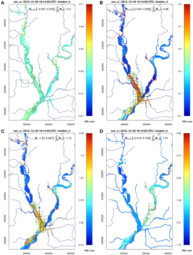
Figure 4. Updated error covariance between the state variable (water level) at Bredon and the state vector (water level elsewhere) at the last assimilation step (7th CSK overpass), for (A) global filter, (B) local filter with Euclidean distance localization, (C) local filter with along-network distance localization, and (D) as (C) but with parameter estimation. Color scales are independent for each plot to ease visualization. The red circle indicates the location of Bredon. The squares are centered at the observation locations, the length of their sides being a symbolic representation of the element of the Kalman gain K_i used to update Bredon at the corresponding assimilation step and filter. The sum of the absolute Kalman gain values for all p observations is indicated by ${\Sigma }^{\text{pi}=1}|K_{\text{i}}|$. Green/red squares are positive/negative gain values (after Garcia-Pintado et al., 2015).

In Figure 4A, the global filter is shown to produce sparsely distributed non-negligible Kalman gain values throughout the domain, with many distant observations influencing the updating at Bredon. The situation is far from what one would expect from a properly constructed assimilation system. Spurious correlations tend to have a dominant effect, leading to relationships which appear unlikely. Moreover, the water levels at observation locations surrounding Bredon have a negative correlation with the level at Bredon, leading to negative gain values (red squares), which are likely to be unphysical.

On the other hand, in Figure 4B the filter with Euclidean distance localization shows a very different situation. The significant Kalman gain values are now much closer to Bredon, and more observations share a fair contribution to the updating. Overall, the spurious correlations seem to have been quite effectively filtered out.

Figure 4C shows that the filter with along-network distance localization seems to be an improved version of the Euclidean distance filter. It does not contain any negative gain values, and there are also a good number of observations with roughly equal high gain values, leading to a robust situation regarding outliers in the WLOs. The distant WLOs in the Severn now have lower gain values, and the highest gain values are closer to Bredon. Overall, this seems the best filter of the three.

The influence of simultaneous inflow and parameter estimation is discussed in the following sections. However, Figure 4D shows the results of a filter similar to the along-network localization filter, but which also includes simultaneous estimation of inflow, global channel friction and distributed bathymetry. This seems to lead to a situation that seems even more physically sound than that of Figure 4C from the point of view of the spatial distribution and share of the Kalman gain values. The higher gain values are now very well distributed around Bredon, and this filter seems to give the best results of all.

Figure 5 shows the time series of water levels predicted by the filter corresponding to Figure 4C (i.e., water levels and joint inflow estimation using along-network distance localization) at Worcester on the Severn. At each assimilation time, the WLOs are used to correct the predicted water levels. While the first satellite overpass misses the peak of the flood, once the SAR data are available, the processing chain is able to successfully adjust the sequential forecast and keep the flood model on track.

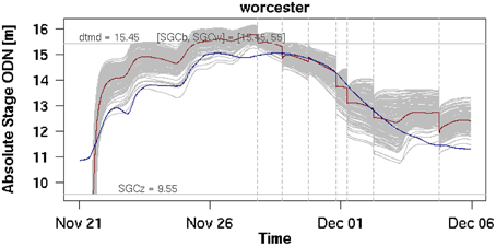
Figure 5. Water level forecast at Worcester, whose major inflows come from Bewdley (river Severn), Kidder Callows (river Stour), and Harford Hill (river Salwarpe). The plot is for a filter configuration involving along-network localization and inflow and parameter estimation. Gray lines are the forecast ensemble, the red line is the mean forecast and the blue line is the gauged water level, used here as a reference and not for modeling or assimilation. Vertical dashed lines indicate the times of the CSK overpasses/assimilation. Horizontal lines indicate the bank level (labeled as “dtmd”), and the mean channel bottom level (labeled as “SGCz”) (after Garcia-Pintado et al., 2015).

Inflow Estimation

A number of filter configurations were compared that performed simultaneous estimation of inflow errors at the times of assimilation, and used these error estimates to correct the inflows from the hydrologic models, assuming a constant bias error forecast model. In this study, the 7 inflow boundary conditions were set from the output of the hydrological models, and no provision was made for lateral inflows along the river network, inflows from smaller tributaries, or groundwater infiltration/exfiltration. These unaccounted inflows/outflows in the flood model may lead to increased/decreased local water levels. Indeed, the satellite-based WLOs may well provide information to improve the estimation of total inflows into the system that are not contained in the prior inflows (i.e., the forecast from the catchment-scale hydrologic models). This fact tended to complicate the analysis somewhat. However, in summary, it was clear that, (a) for the global filter, simultaneous inflow updating promoted ensemble collapse and divergence, and (b) overall the best filter for simultaneous inflow estimation, but without parameter estimation (i.e., friction and bathymetry estimation) was the one with along-network distance localization. This was preferable as a forecast error covariance moderation process, and helped to prevent the development of spurious correlations, which should be adequate for local parameter estimation.

Parameter Estimation

This section focuses on filter configurations with simultaneous friction and/or bathymetry estimation as well as estimation of channel stage and inflows. It was investigated whether these parameters could be simultaneously estimated, and also if this simultaneous estimation lead to an improvement in the flood forecast.

A global Manning's friction coefficient was estimated for the three major channels Severn, Avon, and Teme (the ones with the highest influence on general water levels). The friction coefficient appeared to converge systematically across all the filter configurations. Figure 6 shows this convergence for a filter estimating friction but not bathymetry, but all filters showed similar behavior. However, an important finding was that, despite the likely adequate estimation of channel friction in the major channels, the feedback of friction estimation on the flood forecast within this event seemed negligible.

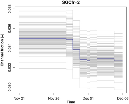
Figure 6. Evolution of the estimate of the global Manning's friction coefficient during the sequential assimilation steps for the three major rivers (Severn, Avon, and Teme) for a filter estimating friction but not bathymetry. Gray lines show the ensemble, and blue line is the mean (after Garcia-Pintado et al., 2015).

Figure 7 shows the evolution of bathymetry during the event for the rivers Severn and Avon and filter configuration in which bathymetry is estimated but not friction (though all filters showed similar behavior). The chainage 0 for the Avon refers to its junction with the Severn, very close to Mythe Bridge. The sequential updating converges systematically toward a profile in which, after the event, the lower part of the Severn is nearly 2 m higher than the prior bathymetry, and the transect between the Saxons Lode and Kempsey gauges is lower than the prior (at some points by 1.5 m). The updating summarizes the influence of the channel conveyance on the flood development. Globally, the SAR WLOs seem to indicate that the prior bathymetry was leading to a model which overestimated the release of water from the flooded domain during the early stages of the event. The sequential increments in the bathymetry along the Avon are also systematic, leading to a raised channel bed profile with respect to the prior. In both rivers, the effect of the localization is clearly visible, as, moving upstream, the increments gradually become smaller as the bed locations move away from the observations. However, as with friction estimation, despite the consistency in bathymetry estimation, the flood forecast did not improve as a result of the updated bathymetry.

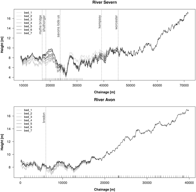
Figure 7. Evolution of the estimate of bathymetry during the seven sequential assimilation steps for the river Severn (top), and the Avon (bottom), for a filter configuration in which bathymetry but not friction was estimated. The ticks at the bottom indicate the location of the available cross sections. The vertical dashed lines and corresponding labels indicate the location of level gauges used for water level validation (after Garcia-Pintado et al., 2015).

Discussion

The study showed that, in a relatively complex scenario with simultaneous uncertain inflows into a flooded domain, a satellite-based forecast of the flood was possible with high accuracy through the assimilation of satellite-derived WLOs into a flood forecast model. However, several aspects needed to be taken into account for a successful operational application of EnKF-based assimilation of WLOs. First, a moderation of the forecast error covariance based on spatial localization was necessary to avoid filter divergence. Second, provided localization was applied, inflow estimation also improved the forecast. Third, the implementation needed to consider the possible uncertainty in model parameters and their simultaneous online estimation.

The study was a hindcasting rather than a forecasting process, as the COSMO-SkyMed constellation (in common with TerraSAR-X) does not provide near real-time geo-registered imagery from which WLOs can be extracted and assimilated to provide a flood forecast. However, other high resolution satellite SARs, specifically RADARSAT-2 and Sentinel-1, do provide near real-time data. The European Space Agency is in the process of launching the Sentinel-1 two-satellite SAR constellation which will give almost daily coverage of floods at European latitudes. The first satellite of the pair was launched in April 2014, and the second is scheduled to follow in 2016. The system allows processed multi-look geo-registered SAR images to be available to the user only an hour or so after download to the ground station. It should therefore be possible to use the techniques developed here to help to provide flood forecasts in near real-time.

Use of Sar-derived Water Level Observations to Improve a Global DTM

Introduction

Many floodplains in the developed world have now been imaged with high resolution airborne LiDAR or InSAR, giving accurate DTMs that facilitate accurate flood inundation modeling. This is not always the case for remote rivers in developing countries. However, the accuracy of DTMs produced for modeling studies on such rivers should be enhanced in the near future by the high resolution TanDEM-X World DEM.

Yan et al. (2015) point out that there was a lack of globally-available DEM data for use as input data for hydraulic modeling before the launch of the Shuttle Radar Topography Mission (SRTM) in 2000. The SRTM DEM covers all land between 60N and 56S, about 80% of the Earth's land surface. Until recently the DEM pixel size has been 3 arc seconds at the equator (about 90 m globally) and 1 arc seconds (about 30 m) in the USA and Australia, thought the latest release data are now 30 m globally. The relative height error ranges from 4.7 to 9.8 m at the continent scale The SRTM heights include vegetation canopy heights so the DEM is not a bare earth DTM. A number of studies have used the SRTM DEM for large-scale hydraulic modeling in river and delta areas (for details see Yan et al., 2015). These have covered many aspects of hydraulic modeling, including water level and water surface slope retrieval, flood extent simulation and water level and discharge prediction. A further near-global DEM which could be used for flood modeling is that produced by the Advanced Spaceborne Thermal Emission and Reflection Radiometer (ASTER). This is a 30 m DEM produced by stereo-photogrammetry, whose second version (ASTER GDEM2) was released in 2011. However the vertical resolution of ASTER GDEM2 ranges from 7 to 14 m and the DEM contains anomalies and artifacts, leading to high elevation errors on local scales and so hampering its use for flood modeling purposes.

The new TanDEM-X DEM produced by DLR (German Aerospace Centre) will produce pole-to-pole coverage with unprecedented accuracy, and should eventually replace the SRTM DEM for large-scale hydraulic modeling. It will have a spatial resolution of 0.4 arc seconds at the equator (10–12 m globally), and a relative height accuracy of less than 2 m on slopes less than 20% and 4 m on slopes greater than 40%. The global DEM is expected to be completed by the end of 2015 (Zink, 2012). Scientific assessment of the DEM is presently at an experimental stage, though there are already assessments of the Intermediate DEM (IDEM), the intermediate product of TanDEM-X based on only one coverage of the globe. Results show that, for the flat and sparsely vegetated terrain found in many floodplains, the IDEM accuracy achieved is better than the design specification (Gruber et al., 2012). As with SRTM, TanDEM-X measures heights to top of canopy so is a Digital Surface Model (DSM) rather than a DTM. However, TanDEM-X combines polarimetric with interferometric measurements to gain additional information from semi-transparent volume scatterers, which will allow extraction of vegetation density and vegetation height (Papathanassiou and Cloude, 2001), potentially aiding the production of a DTM from the DSM. First observations seem to indicate that the TanDEM-X DEM might allow for the first time more detailed local flood studies at the global scale (Yan et al., 2015).

Figure 8A shows a sub-area of the IDEM using airborne LiDAR at 2.5 m resolution. In contrast, Figure 8B shows the SRTM tiles covering the same area at 90 m resolution, the best global DEM that has been available for flood modeling to date. Figure 8C shows the TanDEM-X IDEM tiles for the area, showing the great increase in resolution and accuracy provided by the TanDEM-X global DEM at 12.5 m resolution.

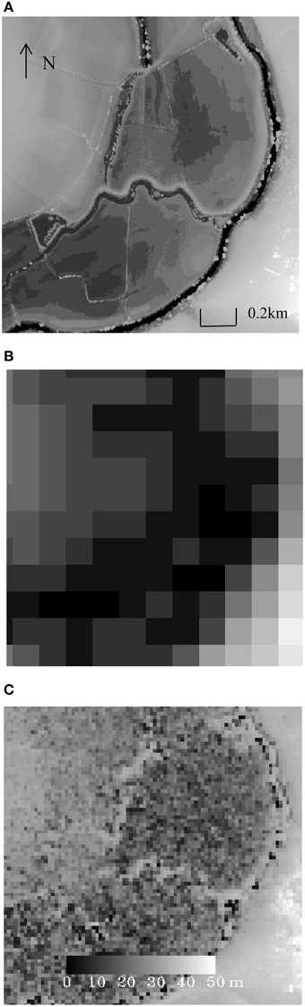
Figure 8. (A) LiDAR DEM of a sub-area of Figure 9 (2.5 m pixels, 1 × 1 km), (B) SRTM DEM (90 m pixels), (C) TanDEM-X IDEM (12.5 m pixels, DLR 2007) (after Mason et al., submitted).

In a related development, increasing use is now being made of flood extents derived from high resolution SAR images for calibrating, validating and assimilating observations into flood inundation models in order to improve these. The model generally uses the SAR images in conjunction with a DEM of the reach, which could be the TanDEM-X DEM. This section discusses an additional use of SAR flood extents to improve the accuracy of the TanDEM-X DEM in the floodplain covered by the flood extents, thereby permanently improving the DEM for future flood modeling studies in this area.

A more accurate DEM would generally result in more accurate modeling and more accurate measurement of WLOs. Though in some cases (e.g., the use of a sub-grid model, e.g., Neal et al., 2012), the TanDEM-X DEM might be spatially averaged to produce a DEM of lower resolution and higher accuracy, in others (e.g., modeling of urban flooding) the full resolution of the TanDEM-X DEM might be required. If it is required to extract WLOs from the SAR flood extents, these would be most accurate using the highest resolution of the TanDEM-X DEM.

The method is based on the fact that for larger rivers the water elevation changes only slowly along a reach, so that the boundary of the flood extent (the waterline) can be regarded locally as a quasi-contour. As a result, heights of adjacent pixels along a small section of waterline can be regarded as a sample of heights with a common population mean. The height of the central pixel in the section can be replaced with the average of these heights, leading to a more accurate height estimate because a substantial portion of the IDEM height error is a random component.

While this will result in a reduction in the height errors along a waterline, the waterline is a linear feature in a two-dimensional space. However, improvements to the DEM heights between adjacent pairs of waterlines can also be made, because DEM heights enclosed by the higher waterline of a pair must be at least no higher than the corrected heights along the higher waterline (otherwise they would emerge from the flood extent), whereas DEM heights not enclosed by the lower waterline must be no lower than the corrected heights along the lower waterline. In addition, DEM heights between the higher and lower waterlines can also be assigned smaller errors because of the reduced errors on the corrected waterline heights. Note that no averaging of height values is performed in correcting heights between waterlines (so that no spatial resolution is lost), whereas the averaging of heights along waterlines is justified because the latter are locally isolines. Full details of the method are given in Mason et al. (submitted).

Study Area and Data Set

The method was tested on a section of the TanDEM-X Intermediate DEM (IDEM) covering an 11 km reach of the Warwickshire Avon, England (Figure 9A). Figure 9B shows the height error map associate with this section of IDEM.

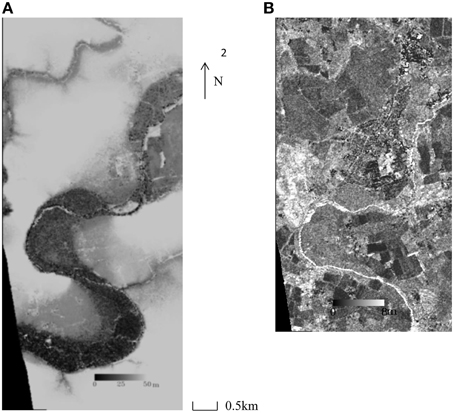
Figure 9. (A) TanDEM-X IDEM of the flooded reach (a sub-area of Figure 1) and, (B) IDEM height error map of the flooded reach (lowest part not supplied) (© DLR 2014) (after Mason et al., submitted).

Flood extents from four of the COSMO-SKyMed images of Figure 2 at various stages of the flood in November 2012 were used (Figure 10).

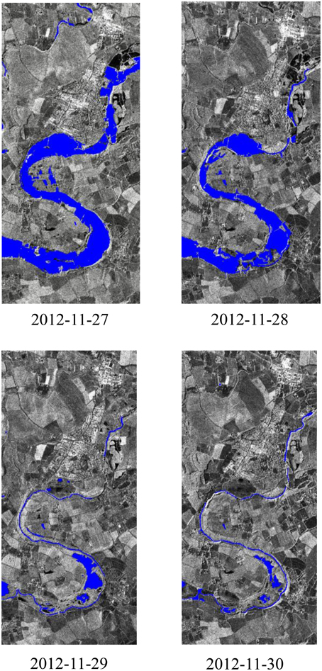
Figure 10. Flood extents (blue) for the event of November 2012 overlain on SAR imagery of the flooded 11 km reach of Figure 9A (© CSK) (after Mason et al., submitted).

Method

Preprocessing

The 12.5 m resolution IDEM and its height error map were re-sampled to the 2.5 m resolution of the CSK images using nearest neighbor interpolation, so that blocks of 5 × 5 pixels in each corrected map contained the same values.

Flood Extent Extraction

Waterlines were detected automatically in the CSK images using the method described in Mason et al. (2012a). No information from the IDEM was used at this stage.

Candidate Waterline Pixel Selection in Rural Areas

Candidate waterline pixels were selected from the flood extent in rural areas. Sections of waterline in the interior of the flood extent caused by regions of emergent vegetation (e.g., hedges) may have erroneously low water levels associated with them. While most of these will have been removed at the segmentation stage, residual sections must be removed prior to further processing. This was facilitated by performing a dilation and erosion operation on the binary flood extent, as described in Mason et al. (2012b).

To cope with the fact that in some regions there were systematic as well as random errors in the IDEM, false positives were further suppressed by selecting waterline points in regions of low or medium DEM slope within a certain height range centered on the mean water height in the area. A waterline point may be heighted more accurately if it lies on a low slope rather than a high slope because any error in its position will cause only a small error in height. The slope threshold was set quite high (0.6) because there was substantial noise in the IDEM slope values due to the large random error in the IDEM heights. In order to find the allowed waterline level range in the area, a histogram was constructed of the waterline levels, and the position of the mean was found. A normal distribution N(μ, σ²) was fitted around the mean μ, and candidate waterline points with levels more than 2.5σ away from μ were suppressed.

Allowance was also made for the fact that the IDEM is a DSM rather than a “bare-earth” DTM. Ideally the IDEM should be processed to remove the heights of surface objects to leave a DTM that can be used in the subsequent processing. This step was approximated in this case by using a land use map to select only candidate waterline pixels in regions of short vegetation, namely grassland and arable classes. It was assumed that any height bias due to failure to remove short vegetation heights would be small compared to the random height error. The majority of the floodplain in the study area was comprised of grassland or arable classes.

Correction of Candidate Waterline Pixel Heights

For each candidate waterline pixel, a window centered on the pixel was examined to select adjacent heights within the window. A window size of 11 × 11 pixels in the 12.5 m IDEM image space was selected as providing a good trade-off between spatial resolution and number of adjacent heights. Because the processing at this stage was in the 2.5 m CSK image space, only one pixel height in each 12.5 m IDEM pixel was selected to avoid introducing spurious height correlations. Provided sufficient surrounding heights were detected, their mean and standard deviation were estimated. If the standard deviation was less than that of the central pixel in the IDEM height error map, the central pixel's height was corrected to be the mean of the surrounding heights, and its IDEM height error map entry was updated.

Adjustment of the IDEM between Adjacent Higher and Lower Waterlines

Each pair of adjacent waterlines was examined sequentially to update the section of IDEM between the current pair of waterlines if possible. The updating process was based on the heights and height errors associated with the candidate waterline pixels on the two waterlines. All IDEM pixels between the waterlines were first modified below the higher waterline of the pair wherever possible. If an IDEM pixel had a height that exceeded that of the nearest candidate waterline pixel on the higher waterline, the IDEM pixel height (h_i) and error (σ_i) were set to those of the waterline pixel (h_w, σ_w). Otherwise, the IDEM pixel height was not modified, but its height error could be reduced to σ_i' if

using

The IDEM pixels between the waterlines were then modified if possible above the lower waterline, using similar rules to the above, in conjunction with the candidate waterline pixel heights and errors of the lower waterline.

An important requirement of the method was that locally the higher waterline of the pair should never be lower than the lower waterline, and to this end lower waterline candidate pixels higher than nearby higher waterline candidate pixels were suppressed in a pre-processing step. In addition, any IDEM pixels enclosed within the lowest waterline boundary were assessed for possible modification to this waterline height. On the other hand, no attempt was made to modify the IDEM outside the boundary of the highest waterline.

Results

On average about 45% of the waterline pixels in each flood extent became candidate pixels able to satisfy the selection criteria of having a low/medium slope, not being a height outlier, and coinciding with short vegetation.

Original and corrected IDEM candidate waterline pixel heights were compared to corresponding airborne LiDAR heights (Table 1). Averaged over the four waterlines considered, it was found that the difference between the original IDEM candidate pixel height and the corresponding LiDAR height had a standard deviation of 1.25 m and a bias of 0.38 m, while for the corrected heights the difference had a standard deviation of only 0.74 m and a similar bias. The corrected heights therefore had a standard deviation only 59% that of the original heights.

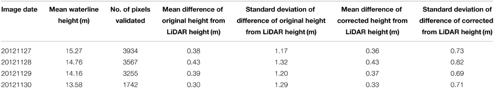
Table 1. Comparison of original and corrected IDEM waterline heights to LiDAR heights.

A floodplain area of 4.3 km² was covered by the waterlines along the 11 km reach. Considering the IDEM pixels between the waterlines, 33% of IDEM heights were above the higher waterline, and 30% below the lower waterline of an adjacent pair (Table 2). When compared to LiDAR, the original higher heights had a mean difference from the LiDAR height of 1.60 m with standard deviation 2.10 m, while after correction the mean difference was 0.19 m with standard deviation 0.86 m. The corrected heights below the lower waterline were similarly improved (see Table 2). Considering the 63% of pixels whose heights were modified in this way, the original heights had a mean difference from the LiDAR of 0.61 m with standard deviation 2.05 m, while after correction the mean difference was 0.26 m with standard deviation 0.74 m. The height errors of a further 23% of IDEM heights between the higher and lower waterlines were also reduced, because of the reduced errors on the corrected waterline heights. The mean error of the original heights was 1.13 m, whereas the mean error of the corrected heights was 0.79 m (Table 3).

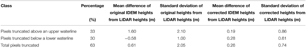
Table 2. Correction of truncated IDEM pixel heights and errors between the waterlines.

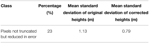
Table 3. Errors for IDEM pixels between the waterlines not truncated but reduced in error.

Discussion

From the above results it can be concluded that the standard deviation and bias of the corrected IDEM heights can be significantly reduced compared to their original counterparts using SAR-derived flood extents. It should also be possible to use the method to improve the final TanDEM-X DEM when this becomes available. This may allow improved large-scale flood inundation modeling with the TanDEM-X DEM in the future.

Although the method presented here has been aimed at improving the TanDEM-X DEM in a river floodplain, it could also be used to improve the DEM in an inter-tidal zone, using a sequence of high resolution SAR images obtained at varying states of the tide between the high and low water marks (e.g., Mason et al., 1999; Thornhill et al., 2012). It could also be applied to a variety of DEMs used for flood inundation modeling other than the TanDEM-X DEM, employing flood extents from higher resolution images at both microwave and optical wavelengths from a variety of satellite and aerial platforms (e.g., SRTM DEM data could be corrected using Sentinel-1 SAR flood extents). The method should also have relevance for the SWOT (Surface Water and Ocean Topography) satellite to be launched in 2020 (JPL, 2015) (see Mason et al., submitted).

Conclusion

These studies have illustrated the utility of a variable-resolution global DEM obtained by combining existing high and low resolution data sets for modeling flood water dynamics globally, at high resolution where possible and at lower resolution over larger rivers in remote areas. They have been based on the symbiosis that exists between DEM data and SAR-derived flood extents.

The two studies have been chosen because they illustrate aspects of two of the main types of hydrologic/hydraulic modeling that are commonly carried out. The variable-resolution DTM is the common denominator linking them. Flood inundation modeling of urban areas requires a high resolution LiDAR DSM and modeling carried out at a local scale, and has been illustrated here using the first example of high resolution SAR-supported flood forecast in river networks. The lower-resolution realization of the DTM could be used for performing global flood modeling, or hydrologic modeling over local areas at lower scales. The second example using SAR-derived WLOs to improve the lower-resolution DTM falls into this category, though is limited to improving the DTM for future modeling studies rather than performing any modeling as such.

The problems to be overcome in constructing a variable-resolution global DTM obviously increase dramatically as the resolution of the data increases. The lower resolution data (e.g., the TanDEM-X WorldDEM) could be sourced from just a few or even one supplier. However, the high resolution data of urban areas would generally be LiDAR data that would have to be licensed from a large number of individual aerial survey companies from all over the world. There are obviously great logistical and implementational difficulties involved in ensuring that low cost high resolution height data can be integrated into the DTM on a global scale, but it is to be hoped that such a DTM may become a reality at some point in the future to aid flood modeling.

Author Contributions

DM wrote the paper, carried out the study on SAR-derived WLOs to improve the TanDEM-X DEM, and was responsible for acquiring the SAR data. JG carried out the study on high resolution SAR-supported flood forecast in river networks, and assisted with the acquisition of the SAR data. HC had overall responsibility for managing the work, assisted with the acquisition of the SAR data, reviewed the manuscript and gave approval for publication. SD assisted with the data assimilation theory and provided a critical review of the manuscript.

Conflict of Interest Statement

The authors declare that the research was conducted in the absence of any commercial or financial relationships that could be construed as a potential conflict of interest.

Acknowledgments

This work was supported by NERC through the DEMON project (NE/I005242/1) within the NERC SRM (Storm Risk Mitigation) programme, and the SINATRA project (NE/K00896X/1) within the NERC FFIR (Flooding From Intense Rainfall) programme. The authors are grateful to DLR for the provision of the TanDEM-X IDEM data. We thank the EA for the precipitation and standard flow/level gauge datasets. Thanks are due to Moira Mason for assistance with the satellite image acquisition.

References

Allan, R. P., and Soden, B. J. (2008). Atmospheric warming and the amplification of precipitation extremes. Science 321, 1481–1484. doi: 10.1126/science.1160787
Bates, P. D., and De Roo, A. (2000). A simpled raster-based model for flood inundation simulation. J. Hydrol. 236, 54–77. doi: 10.1016/S0022-1694(00)00278-X
Beven, K., Cloke, H., Pappenberger, F., Lamb, R., and Hunter, N. (2015). Hyperresolution information and hyperresolution ignorance in modelling the hydrology of the land surface. Sci. China Earth Sci. 58, 25–35. doi: 10.1007/s11430-014-5003-4
Bierkens, M. F. P., Bell, V. A., Burek, P., Chaney, N., Condon, L., David, C. H., et al. (2015). Hyper-resolution global hydrological modelling: what is next? Hydrol. Process. 29, 310–320. doi: 10.1002/hyp.10391
Donigian, A., Bicknell, B. R., and Imhoff, J. C. (1995). “Hydrological simulation program – fortran (hspf),” in Computer Models of Watershed Hydrology, ed V. Singh (Littleton, CO: Water Resources Publications), 395–442.
Durand, M., Neal, J. C., Rodriguez, E., Andreadis, K. M., Smith, L. C., and Yoon, Y. (2014). Estimating reach-averaged discharge for the river Severn from measurements of river water surface elevation and slope. J. Hydrol. 511, 92–104. doi: 10.1016/j.jhydrol.2013.12.050
Eineder, M., Fritz, T., Jaber, W., Rossi, C., and Breit, H. (2012). “Decadal earth topography dynamics measured with TanDEM-X and SRTM,” in Proceedings of IEEE International Geoscience and Remote Sensing Symposium (Munich). doi: 10.1109/igarss.2012.6351130
Evensen, G. (1994). Sequential data assimilation with a nonlinear quasi-geostrophic model using Monte Carlo methods to forecast error statistics. J. Geophys. Res. 99, 10143–10162. doi: 10.1029/94JC00572
Friedland, B. (1969). Treatment of bias in recursive filtering. IEEE Trans. Autom. Control 14, 359–367. doi: 10.1109/TAC.1969.1099223
Garcia-Pintado, J., Mason, D. C., Dance, S. L., Cloke, H. L., Neal, J. C., Freer, J., et al. (2015). Satellite-supported flood forecast in river networks: a real case study. J. Hydrol. 523, 706–724. doi: 10.1016/j.jhydrol.2015.01.084
Garcia-Pintado, J., Neal, J. C., Mason, D. C., Dance, S., and Bates, P. (2013). Scheduling satellite-based SAR acquisition for sequential assimilation of water level observations into flood modelling. J. Hydrol. 495, 252–266. doi: 10.1016/j.jhydrol.2013.03.050
Gruber, A., Wessel, B., Huber, M., Breunig, M., Wagenbreener, S., and Roth, A. (2012). “Quality assessment of first TanDEM-X DEMs for different terrain types,” in 9th European Conference on Synthetic Aperture Radar (Nuremberg), 101–104.
Hamill, T. M., Whitaker, J. S., and Snyder, C. (2001). Distance-dependent filtering of background error covariance estimates in an Ensemble Kalman filter. Mon. Wea. Rev. 129, 2776–2790. doi: 10.1175/1520-0493(2001)129<2776:DDFOBE>2.0.CO;2
Hunt, B. R., Kostelich, E. J., and Szunyogh, I. (2007). Efficient data assimilation for spatiotemporal chaos: a local ensemble transform Kalman filter. Phys. D 230, 112–126. doi: 10.1016/j.physd.2006.11.008
JPL. (2015). SWOT: The Surface Water and Ocean Topography Mission, eds, L.-L. Fu, D. Alsdorf, R. Morrow, and E. Rodriguez. Available online at: https://swot.jpl.nasa.gov/files/swot/SWOT_MSD_1202012.pdf
Kirchgessner, P., Nerger, L., and Bunse-Gerstner, A. (2014). On the choice of an optimal localization radius in ensemble Kalman filter methods. Mon. Wea. Rev. 142, 2165–2175. doi: 10.1175/MWR-D-13-00246.1
Mason, D. C., Amin, M., Davenport, I. J., Flather, R. A., Robinson, G. J., and Smith, J. A. (1999). Measurement of recent intertidal sediment transport in Morecambe Bay using the waterline method. Estuarine Coast. Shelf Sci. 49, 427–456. doi: 10.1006/ecss.1999.0508
Mason, D. C., Davenport, I. J., Neal, J. C., Schumann, G. J.-P., and Bates, P. D. (2012a). Near real-time flood detection in urban and rural areas using high resolution Synthetic Aperture Radar images. IEEE Trans. Geosci. Remote Sens. 50, 3041–3052. doi: 10.1109/TGRS.2011.2178030
Mason, D. C., Garcia-Pintado, J., and Dance, S. L. (2014). Improving flood inundation monitoring and modelling using remotely sensed data. Civ. Eng. Surveyor 2014, 34–37.
Mason, D. C., Schumann, G. J.-P., Neal, J. C., Garcia-Pintado, J., and Bates, P. D. (2012b). Automatic near real-time selection of flood water levels from high resolution Synthetic Aperture Radar images for assimilation into hydraulic models: a case study. Remote Sens. Environ. 124, 705–716. doi: 10.1016/j.rse.2012.06.017
Matgen, P., Montanari, M., Hostache, R., Pfister, L., Hoffman, L., Plaza, D., et al. (2010). Towards the sequential assimilation of SAR-derived water stages into hydraulic models using the particle filter: proof of concept. Hydrol. Earth Sys. Sci. 14, 1773–1785. doi: 10.5194/hess-14-1773-2010
Neal, J. C., Schumann, G. J.-P., and Bates, P. D. (2012). A subgrid channel model for simulating river hydraulics and floodplain inundation over large and data sparse areas. Water Resour. Res. 48:W11506. doi: 10.1029/2012wr012514
Papathanassiou, K. P., and Cloude, S. R. (2001). Single-baseline polarimetric SAR interferometry. IEEE Trans. Geosci. Rem. Sens. 39, 2352–2363. doi: 10.1109/36.964971
Pappenberger, F., Dutra, E., Wetterhall, F., and Cloke, H. L. (2012). Deriving global flood hazard maps of fluvial floods through a physical model cascade. Hydrol. Earth Syst. Sci. 16, 4143–4156. doi: 10.5194/hess-16-4143-2012
Petrie, R. E., and Dance, S. L. (2010). Ensemble-based data assimilation and the localisation problem. Weather 65, 65–69. doi: 10.1002/wea.505
Raclot, D. (2006). Remote sensing of water levels on floodplains: a spatial approach guide by hydraulic functioning. Int. J. Rem. Sens. 27, 2553–2574. doi: 10.1080/01431160600554397
Roux, H., and Dartus, D. (2008). Sensitivity analysis and predictive uncertainty using inundation observations for parameter estimation in open-channel inverse problem. J. Hydr. Eng. 134, 541–549. doi: 10.1061/(ASCE)0733-9429(2008)134:5(541)
Schumann, G. J.-P., Bates, P. D., Neal, J. C., and Andreadis, K. M. (2014). Fight floods on global scale. Nature 507, 169. doi: 10.1038/507169e
Schumann, G. J.-P., Neal, J. C., Mason, D. C., and Bates, P. D. (2011). The accuracy of sequential aerial photography and SAR data for observing urban flood dynamics: a case study of the UK summer 2007 floods. Rem. Sens. Environ. 115, 2536–2546. doi: 10.1016/j.rse.2011.04.039
Smith, P. J., Thornhill, G. D., Dance, S. L., Lawless, A. S., Mason, D. C., and Nichols, N. K. (2013). Data assimilation for state and parameter estimation: application to morphodynamic modelling. Q. J. R. Meteorol. Soc. 139, 314–327. doi: 10.1002/qj.1944
Thornhill, G. D., Mason, D. C., Dance, S. L., Lawless, A. S., and Nichols, N. K. (2012). Integration of 3D Variational Data Assimilation with a coastal area morphodynamic model. Coast. Eng. 69, 82–96. doi: 10.1016/j.coastaleng.2012.05.010
Yan, K., Di Baldassarre, G., Solomatine, D. P., and Schumann, G. J.-P. (2015). A review of low-cost space-borne data for flood modelling: topography, flood extent and water level. Hydrol. Processes 29, 3368–3387. doi: 10.1002/hyp.10449
Keywords: digital terrain model, flood extent, Synthetic Aperture Radar, flood modeling, data assimilation
Citation: Mason DC, Garcia-Pintado J, Cloke HL and Dance SL (2015) The potential of flood forecasting using a variable-resolution global Digital Terrain Model and flood extents from Synthetic Aperture Radar images. Front. Earth Sci. 3:43. doi: 10.3389/feart.2015.00043
Received: 27 April 2015; Accepted: 24 July 2015;
Published: 06 August 2015.
Edited by:
Guy Jean-Pierre Schumann, University of California, Los Angeles, USAReviewed by:
Tim Van Emmerik, Delft University of Technology, NetherlandsPatrick Matgen, Luxembourg Institute of Science and Technology, Luxembourg
Copyright © 2015 Mason, Garcia-Pintado, Cloke and Dance. This is an open-access article distributed under the terms of the Creative Commons Attribution License (CC BY). The use, distribution or reproduction in other forums is permitted, provided the original author(s) or licensor are credited and that the original publication in this journal is cited, in accordance with accepted academic practice. No use, distribution or reproduction is permitted which does not comply with these terms.
*Correspondence: David C. Mason, Department of Geography and Environmental Science, University of Reading, Russell Building, Whiteknights, PO Box 227, Reading RG6 6AB, Berkshire, UK, d.c.mason@reading.ac.uk