Using the Ocean Health Index to Identify Opportunities and Challenges to Improving Southern Ocean Ecosystem Health
 Catherine S. Longo1
  Melanie Frazier2
  Scott C. Doney3
  Jennie E. Rheuban3
  Jennifer Macy Humberstone4,5
  Benjamin S. Halpern2,5,6*
- 1Marine Stewardship Council, Marine House, London, UK
- 2National Center for Ecological Analysis and Synthesis, University of California, Santa Barbara, Santa Barbara, CA, USA
- 3Marine Chemistry and Geochemistry, Woods Hole Oceanographic Institution, Woods Hole, MA, USA
- 4SCS Global Services, Emeryville, CA, USA
- 5Bren School of Environmental Science and Management, University of California, Santa Barbara, Santa Barbara, CA, USA
- 6Faculty of Natural Sciences, Department of Life Sciences (Silwood Park), Imperial College London, Ascot, UK
The Antarctic coast and seas are considered some of the most pristine marine systems on Earth. Their comprehensive assessment is critical because meeting ambitious conservation objectives while maintaining sustainable human uses will be increasingly challenging with growing climate change impacts, recovery from past overharvesting, and potential revision of activities permitted with future revisions of the existing governance structure. We used the Ocean Health Index (OHI) to deliver an integrated assessment of the Antarctic marine ecosystems' evolving ecological and social dimensions. The OHI provides a framework to evaluate sustainable delivery of benefits people want from healthy oceans by measuring progress toward 10 widely-held societal goals. These goals include, conservation objectives, as well as other objectives, so as to identify tradeoffs across multiple priorities. We adapted the Index to the unique aspects and data availability of Antarctica. OHI scores were calculated for each sub-region defined by the Convention for the Conservation of Antarctic Marine Living Resources (CCAMLR) as well as the region overall. OHI scores for conservation-related goals (biodiversity, clean water) were generally high, though with some stressor impacts (i.e., climate-driven decline of sea-ice, and pathogen pollution). However, a sensitivity test on the sea-ice habitat indicator showed biodiversity scores might be much lower in the vicinity of the Antarctic Peninsula. Preservation of lasting special places, captured in the sense of place sub-goal, scored relatively low due to limited extent of Marine Protected Areas in the Southern Ocean. In several cases, scores are low due to under-utilization of resources, rather than environmentally unsustainable practices (e.g., food provision, natural products, tourism, and recreation). However, increased human activities would intensify the risk of pollution, pathogen contamination, and disturbance to wildlife, particularly if compounded with future climate change impacts. Therefore, scores may reflect the need to select more conservative targets for human use, articulated in international treaties, taking future risks into account. Our results highlight the need for more research on both natural and social science aspects of the Antarctic system, as well as the need to evaluate targets under different scenarios, so as to provide robust science-based advice for future decision-making in the region.
Introduction
Marine systems are affected by anthropogenic stressors worldwide (Halpern et al., 2008, 2015a), and many of these human pressures are increasing with time (Halpern et al., 2015a). Even one of the most inaccessible regions, the Southern Ocean, is no longer pristine. Anthropogenic stressors reported in the region include local and remote sources of debris, contaminants, oil leaks, and alien species (Tin et al., 2009; Aronson et al., 2011); lingering effects of historical whaling (Ainley et al., 2010; Surma et al., 2014); legal, illegal, and unregulated fishing (Ainley and Pauly, 2014; Österblom et al., 2014); wildlife disturbance from tourism and scientists (Tin et al., 2009; Aronson et al., 2011; Ainley and Pauly, 2014); as well as, perhaps most importantly, climate change (Schofield et al., 2010; Doney et al., 2012; Chown et al., 2015).
The Antarctic Treaty System (ATS), the set of multi-national agreements governing the continent and the surrounding ocean poleward of 60°S since 1961, explicitly recognizes the existence, aesthetic, and scientific value of Antarctica (http://www.ats.aq/e/ats.htm). The Protocol on Environmental Protection to the Antarctic Treaty (Madrid, 1991) defines the whole of Antarctica “as a natural reserve, devoted to peace and science.” At the same time, the ATS allows and regulates human activities in the region, including tourism, fishing, marine mammal harvest, and permanent settlements tied to scientific missions. While conservation is a priority, the international community also clearly recognizes that a healthy Antarctic system includes people and provides a broad range of societal goals. Here we ask whether these goals are being satisfied, whether they are being pursued sustainably, and what future data collection and governance priorities for the region should be.
In order to do so, a comprehensive and integrated assessment of ecological and social dimensions of ocean health for the Antarctic is needed. The Ocean Health Index (OHI) provides a useful framework for such an integrated assessment (Halpern et al., 2012, 2015b). The OHI evaluates how well marine systems sustainably deliver 10 widely held societal goals that people have for healthy oceans. The index assesses goals related to human use (e.g., food provision from fisheries, natural products extraction, and tourism and recreation) as well as conservation objectives (e.g., clean waters and biodiversity). Because the index captures ecological and socio-economic aspects of ecosystem health simultaneously, rather than treating them as separate or independent, it provides a key tool for producing the integrated evaluations required for ecosystem-based management.
The OHI is explicitly quantitative, calculated by combining individual indicators via a structured framework designed to measure progress toward each of the 10 goals (4 of which are further subdivided in sub-goals). Each goal/sub-goal is assessed for its current state, measured against a reference point representing its full, sustainable delivery, i.e., a score of 100, as well as its recent trend, existing cumulative pressures that negatively impact its delivery, and resilience characteristics that can respond or mitigate those pressures (Halpern et al., 2012). The index is designed to represent the health of the system through a human lens, because communicating ecosystem health in terms of losses and gains in benefits that people value is a powerful communication tool for managers and wider audiences. Importantly, describing the ecosystem in terms of benefits allows for simultaneously evaluating intangible benefits, such as sense of place, as well as economic benefits, such as revenues from marine sectors, and ecosystem provisioning and supporting services, such as food provision and biodiversity preservation. Nevertheless, with this type of approach it is crucial to set targets and reference points appropriately for each of the components of the index, so as to capture societal objectives that are compatible with the system's carrying capacity and resilience (Samhouri et al., 2012).
The index is not designed to capture long-term sustainability issues, since these are not likely to be adequately estimated through a static indicator that assumes “business as usual” characteristics of the system. Instead it uses current data and indicators to anticipate the near-term future state of the goal as an indication of sustainability (Halpern et al., 2012). Longer-term projections of ocean health are better evaluated through dynamic mechanistic models.
To assess the condition of Antarctica's ocean and coastal regions, we calculated OHI scores by adapting the existing OHI framework to the particular characteristics of the Antarctic region, using regionally specific data-sets and established benchmarks. Environmental preservation is one of multiple goals for management; however, conservation priorities may be deemed particularly important for Antarctica. In conducting a tailored OHI assessment for Antarctica, we aim to inform ongoing discussions on how to use or protect Southern Ocean resources (e.g., Jacquet and Brooks, 2015; Jacquet et al., 2016). Because the OHI is designed to capture the tradeoffs across a complete range of, often conflicting, societal goals for healthy oceans, it also provides a framework to evaluate and discuss the relative importance of different goals. Ultimately, this information can be used to establish goal targets that better reflect our values. These Index scores are an effective decision-support tool because they can be clearly communicated to a broad audience and importantly, a variety of resources and tools (Lowndes et al., 2015; http://ohi-science.org/resources/tools/) exist to facilitate updating scores every year so changes over time can be monitored. Additionally, we use this exercise to identify what information would contribute to more reliable future assessments.
Materials and Methods
Here, we provide a brief overview of the OHI framework, however, methods for calculating the Index, and the conceptual framework and rationale for how it is constructed, are detailed extensively elsewhere (Halpern et al., 2012, 2015b; ohi-science.org).
The Ocean Health Index (Halpern et al., 2012, 2015b) evaluates a broad range of benefits and services that people value and want from healthy oceans. These are assessed globally as 10 widely held public goals for ocean ecosystems, four of which are further subdivided into two sub-goals (Table 1). Goals are scored on a scale of 0–100, with 100 being the best possible score. Each goal score, Gi, is calculated as the average of current status, xi, and the likely future status, :
where current status is a measure of the current performance relative to a reference value that represents the maximum sustainable performance of that goal. Likely future state is intended to capture whether status is likely to increase or decrease in near term, and is calculated as:
Likely future status takes into account: recent trends in status, Ti, calculated using a linear regression model of the change in status as a function of time, in years; known pressures, pi, that threaten the delivery of each goal (scaled from 0 to 1, with 1 being the worst possible score predicted to negatively affect goal scores); and resilience factors, ri, that can mitigate those stressors (scaled from 0 to 1, with 1 being the best possible score predicted to positively affect goal scores). The assumption is that, under current conditions, the status will continue on its recently observed trajectory, i.e., its recent trend, but stressors and resilience can modify that trajectory up or down, depending on which is strongest. Ti is then the slope of the regression model multiplied by 5, corresponding to the estimated future status 5 years from now, under current conditions, to which then the ri and pi modifiers are applied. A weighting factor, β, establishes the relative importance of the trend versus resilience and pressure factors in influencing the likely future state score. Following previous assessments (e.g., Halpern et al., 2012), we used β = 0.67 to give the trend twice as much importance as the pressure and resilience scores, as it is considered a more reliable indicator of near future state because it directly captures the goal's historical status change. The assumption that the recent trend contains more information about the likely near future state is based on expert opinion, in the absence of a better understanding of the mechanistic interactions between these variables. Note that we do not include a discount rate because, on a short-term horizon, it is generally set to 0; however, it may be incorporated into the calculation if desired (Halpern et al., 2012). Because these are indicators based on best current knowledge, and not mechanistic predictive models, they work best on a short time horizon where departure from currently observed conditions is less likely. For this reason a short timeframe of 5 years was chosen for the likely future state.
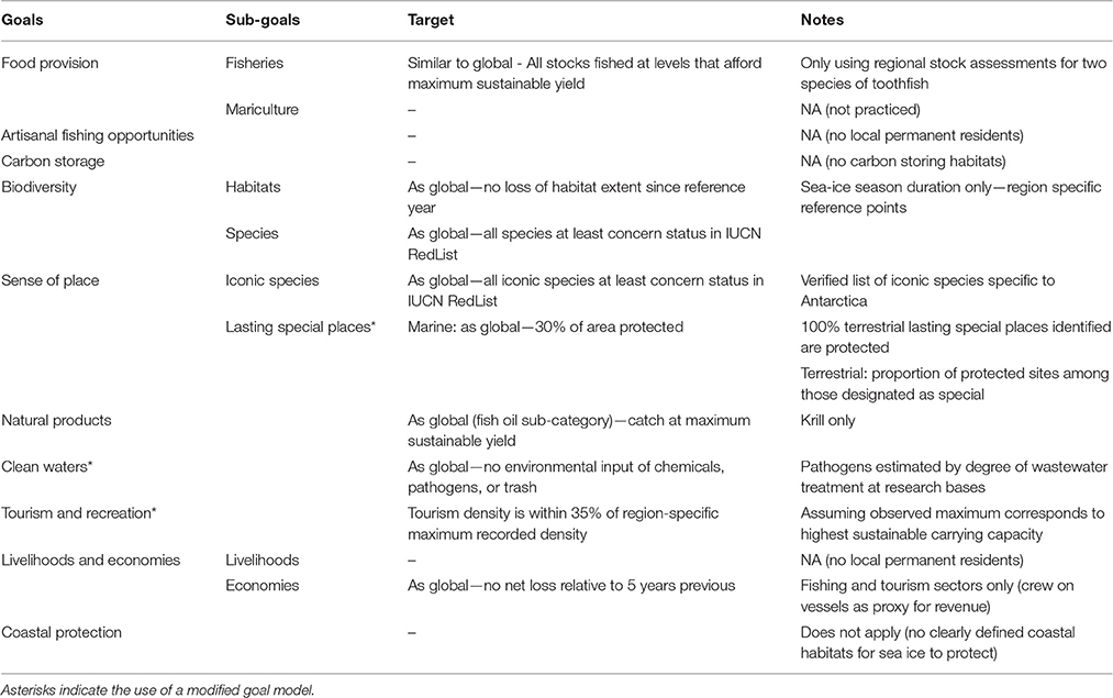
Table 1. Differences between Antarctica and global goal models.
To obtain each region's overall Index score, goal scores were averaged, which assumes all goals are equally important. Goals are all given equal weights when there is no information on the relative societal importance of the goals. These individual subregion index scores were then averaged using an area-weighted mean to derive an overall score for the Antarctica region.
Given the composite nature of the index, and the high number of data-sets, models, parameters, weights, and assumptions required for its calculation, it is very challenging to evaluate the uncertainty associated to the estimation of the goals or the overall index. Although an approach was developed to capture risk of error associated with poor data quality, by using as proxy the degree to which a score relies on gap-filled data (i.e., indirectly derived or modeled), this is mainly suited for large scale applications of the Index, and only addresses one type of source of uncertainty (Frazier et al., 2016). Here, we try to address these concerns by thoroughly documenting the data sources and methods in the Supplement, and discussing the main caveats to the interpretation of the scores.
We describe below, the data and general methods we used to estimate status/trend, pressures, and resilience components of the OHI model for Antarctica.
Study Area
We used the boundaries of the Food and Agricultural Organization of the United Nations (FAO) major fishing areas identified in Antarctica as larger reporting regions (Figure 1). These regions coincide with those monitored under the Convention for the Conservation of Antarctic Marine Living Resources and the associated Commission (CCAMLR, CCAMLR, 2014a). CCAMLR statistical regions extend equatorward beyond the 60°S jurisdictional boundary of the Antarctic Treaty, thus they incorporate some international waters as well as areas belonging to other exclusive economic zones (EEZs). These EEZs were assessed elsewhere (Halpern et al., 2015b; ohi-science.org) and thus are excluded from the results presented here. Each larger region was further divided into sub-regions according to CCAMLR data sampling and reporting sub-regions (Atlantic sub-regions coded 48.X, Indian 58.X, and Pacific 88.X) (Figure 1). This choice allows for comparability with CCAMLR studies and matches the resolution of available data and management units.
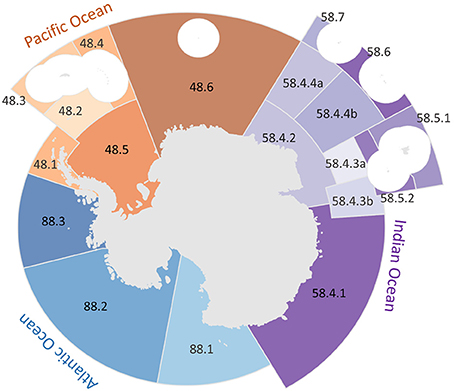
Figure 1. CCAMLR region boundaries. CCAMLR areas are identified by color group: blue regions are located in the Pacific Ocean, orange in the Atlantic Ocean, and purple in the Indian Ocean. We calculated scores for each of the CCAMLR sub-areas, which are differentiated by shading. Area codes follow CCAMLR naming conventions with the first two digits identifying the FAO region and following numbers specific to the CCAMLR sub-areas. White circles are EEZ areas of island regions that were not included because they were analyzed in the Ocean Health Index global assessment.
Modifications to Global OHI
One of the strengths of the OHI is that it can be adapted to the specific needs of an assessment region. If a goal is not relevant to a specific location, it can be omitted from the calculation of the Index. In the case of Antarctica, several goals did not apply anywhere in the study region, while others were only relevant for specific sub-regions. For the Antarctic region, we thus focus on a regionally relevant subset of seven OHI goals and six corresponding sub-goals. For each subregion within Antarctica, a score for each of the seven goals, Gi, and, where applicable, for the sub-goals, is calculated. Further details on what was excluded, and why, are provided under Section Goal status calculations.
The models used to calculate goal status scores were similar to those used in the most recent Ocean Health Index (2015) global assessment (Halpern et al., 2012, 2015b). However, the Antarctic region is distinct from the rest of the world's EEZs, and the models and data were tailored to accommodate the region's unique characteristics (Table 1). Three key factors drove decisions about how OHI goal models were adapted, the first two relating to social aspects and the third stemming from bio-physical properties: (1) Antarctica has no indigenous residents, (2) the governing authority is distributed across multiple nations, and (3) there is higher exposure and sensitivity to climate change drivers due to species' highly specialized traits and presence of sea-ice as a key habitat (Aronson et al., 2011 and references therein). Changes made for this study are briefly described below, and detailed in the Supplementary Materials.
An important aspect of calculating an indicator for goal status is defining the indicator's reference point, which is the value of the indicator that is assumed to correspond to a fully achieved goal, and thus a perfect score. The choice of reference points is thus fundamental to interpreting each goal score as well as the overall index score. The types of reference points used for each goal and sub-goal are consistent with those in Halpern et al. (2015a), but the way that reference points were defined changed in a few goals and sub-goals based on the availability of better data or a region-specific understanding of how to determine appropriate reference points (Table S1).
Goal Status Calculations
This section describes the calculations for the status and trend (i.e., recent change in status) components of the goals calculated for the Antarctica assessment.
Food Provision
The food provision goal is meant to capture whether the seafood provisioning potential of the region is utilized to its full sustainable potential, through wild or cultured harvest. The assumption is that food provision is a global priority, so it is important to maximize sustainable harvest, regardless of whether it is consumed locally. This goal does not however take into account more complex issues surrounding unequal access to these resources (captured instead in the artisanal opportunities goal) and food security. The goal is measured through two sub-goals, one for wild capture harvest, the fisheries sub-goal, and one for cultured harvest, the mariculture sub-goal.
Food provision: fisheries sub-goal
The fisheries sub-goal captures whether fisheries are being exploited to their maximum sustainable yield (MSY), while being managed with adequate precaution. Status for this sub-goal was calculated using the ratio of current catch to the legally set, region-specific catch limit (i.e., the reference point) for each of the relevant fishery stocks. For Antarctic fisheries, commercial harvest is only allowed for four species (i.e., two toothfish species, mackerel ice-fish, and krill), all of which have formal stock assessments. Since krill is not sold for direct food provision, it was evaluated within the natural products goal (see below). Mackerel ice-fish is only found in the EEZ's of South Georgia Island and Heard Island, both outside the area covered by this study, and was not included. The calculation of the food provision status is therefore derived only from the catches of the Antarctic (Dissostichus mawsoni), and Patagonian (Dissostichus eleginoides) toothfish species. There are a few by-catch species for which legal catch limits exist. However, these represent conservation measures rather than food provision targets, such that the management objective is to catch as little as possible and harvest cannot be landed. Therefore, catching those species would not contribute to food provision. As such, non-target species were not included in the food provision calculation.
There is known under-reporting of toothfish catches due to illegal fishing (Agnew et al., 2009; Österblom et al., 2010). There have been previous attempts on the part of the Working Group for Fish Stock Assessment at quantifying illegal catches of toothfish, particularly in the Indian Ocean Sector of the Convention Area. These estimates however are not considered reliable and thus are no longer reported (SC-CAMLR-XXIX). Thus, we could not quantify or fully account for this in measuring the status of food provision. However, this aspect is taken into consideration by managers in setting regional targets or, in some cases, fisheries closures. Thus, we account for this within the fisheries management score that was used for the resilience calculation (see Supplementary Materials). For details on how the catch time-series data were treated, see Supplementary Materials.
Food provision: mariculture sub-goal
The mariculture sub-goal was excluded because there is no mariculture in Antarctica at present or in the planned future. The “food provision” goal is thus equivalent to the “fisheries” sub-goal.
Artisanal Fishing Opportunities
This goal is intended to capture the desire to maintain access to sustainable coastal fishing resources for small-scale commercial, subsistence, or traditional practices. Although some artisanal harvest is allowed to support scientific expeditions, this is not pursued in any measurable amount in Antarctica, so this goal was not evaluated.
Carbon Storage
The Carbon Storage goal, as defined in the global OHI, is measured through the level of preservation of coastal habitats that have long-term carbon storage properties, such as mangroves, seagrasses, and wetlands (i.e., not corals or seaweed because in that case there is no long-term net positive storage). The objective is to quantify short-term changes in carbon reservoirs that are directly attributable to human management and protection, or lack thereof, leading to habitat degradation and carbon release. The carbon storage goal is excluded in our analysis because none of the coastal habitats that provide this service are present in Antarctica. Carbon storage, as represented in the OHI goal, differs from carbon storage in the open-ocean that is governed by a combination of the solubility and biological pumps. The Southern Ocean in particular contributes a substantial fraction of the net global ocean carbon uptake of anthropogenic carbon dioxide associated with basin-scale upwelling of old subsurface waters (Khatiwala et al., 2013). This form of carbon storage service offered by the water column is not included in either the global or Antarctic OHI for two reasons: (1) the oceanic uptake of anthropogenic carbon dioxide is controlled primarily by physical chemistry and large-scale ocean circulation and thus is not directly responsive to human management (other than through global mitigation approaches such as reducing carbon dioxide emissions to the atmosphere) (Doney et al., 2014); and (2) uptake of anthropogenic carbon dioxide leads to ocean acidification, with the potential for negative impacts on several different taxa, including coral and mollusks, and thus, does not represent a sustainable long-term carbon storage service (Doney et al., 2009).
Coastal Protection
The Coastal Protection goal is intended to capture coastal protection of habitats in the water and fringing the coastline, but not habitats that are considered inland. The coastal protection goal was excluded because there are no well-delimited coastal Antarctic habitats to protect from erosion and inundation and essentially no human structures along the coast that would be at risk from coastal erosion. Indeed it is true that sea-ice melting entails reduced protection of sea-ice itself as a coastal habitat. However, the key habitat for most of the Antarctic food-web is really the sea-ice edge, while the sea-ice surface far from the edge is used as a habitat by a handful of species. Moreover the health of sea-ice related ecosystems is already captured in the sea-ice indicator used to calculate the Habitats sub-goal. Using the same indicator for this goal would result in double-counting.
Biodiversity
The biodiversity goal is meant to capture the desire to preserve biodiversity for future generations for its aesthetic, existence, as well as supporting service values. It is measured through two proxies, species status and habitat health, which are meant to be complementary indicators.
Biodiversity: habitats sub-goal
For the global analysis (Halpern et al., 2012, 2015a), the status of the habitats sub-goal is calculated as current habitat area or, when possible, habitat quality compared to a historical benchmark. The only habitat assessed in this study was sea-ice because insufficient data exist for any other habitats (e.g., benthic communities). Annual sea-ice season duration was used as a proxy for habitat health, following Stammerjohn et al. (2008, 2012), using the number of days between ice advance and ice retreat. Ice season duration takes into account both changes in sea-ice extent and the length of the ice season, as ice-free areas are given a value of zero for ice season. Because ice-season varies across the CCAMLR regions, we defined region-specific reference points as the mean of the ice season during the first decade of available data (1980–1989).
Biodiversity: species sub-goal
The status of the species sub-goal was calculated using global OHI data and methods (Halpern et al., 2012). The reference point for this sub-goal is to have all species at a risk status of Least Concern, and status is scaled to equal 0 when 75% of species are extinct, a level comparable to the five documented mass extinctions. The conservation status of each species is based on the species-specific risk categories (e.g., vulnerable, not threatened) reported by the International Union for Conservation of Nature (IUCN, 2015), which is converted to a numerical score (Table S2). Species distributions are determined using IUCN and Aquamap (Kaschner et al., 2015) species range maps. The species scores are averaged for each 0.5 degree raster, and then, the raster scores are averaged for each region (adjusting for the area of the raster cell). Individual populations may have experienced significant declines, which may affect ecosystem functioning, but as long as they are viable (i.e., of least concern status) the goal will score well.
Sense of Place
The sense of place goal is meant to capture the desire to preserve areas and species that contribute to people's connectedness to the oceans, and hold a socio-cultural value for local communities that might have traditions tied to their existence, or are iconic and valued for their existence by people who may never experience them directly (e.g., the Great Barrier Reef, blue whales, etc).
Sense of place: iconic species sub-goal
This sub-goal was calculated using the same methods as the global OHI assessment. The average conservation status (i.e., IUCN data converted to a numerical score) is calculated for all the species within a region that have iconic significance, due to social or ecological reasons. The reference point for this sub-goal is to have all species at a risk status of Least Concern. In the Antarctic region, we identified 32 iconic species (Table S2). As described for the species diversity sub-goal, this goal is assessed independently of any loss of functional role of these species in the ecosystem.
Sense of place: lasting special places sub-goal
This goal was calculated using the same methods as the global OHI assessment, except the reference point for marine lasting special places was 30% of the entire CCAMLR region (vs. 3 nm offshore). The benchmark of 30% was chosen as a relatively arbitrary reference point (Halpern et al., 2012). The goal for terrestrial lasting special places (1 km inland) was assigned a perfect score of 100 because the ATS has a regulatory process whereby any place identified as special by any member country is given protected status. The relative contribution of land versus water was equally weighted, so the lasting special places status scores was the average of these two scores within each CCAMLR region. Although the whole Antarctic region may be considered a lasting special place, according to the Antarctic Treaty System, we deemed it appropriate to focus on areas with special designation because they exist and there have been strong debates on creating additional ones (Jacquet and Brooks, 2015), suggesting that some areas are viewed as particularly important for the conservation of Antarctic ecosystems.
Natural Products
This goal captures whether natural products for which there is demand are harvested to their full, sustainable potential. The only natural product assessed in Antarctica is the krill fishery, which produces krill oil and krill meal. Status is calculated in the same way as the fisheries sub-goal, using the ratio of current reported krill catch to the current precautionary catch limit (i.e., the goal reference point). The total allowable catch takes into account krill biomass that needs to be reserved for the consumption of the other predators in the food-web. A status score is computed for each CCAMLR region where krill catch is reported.
Clean Waters
The goal for clean waters is to maintain them free of contamination, pathogens, and anthropogenic toxic algal blooms or anoxia for people to enjoy as well as for environmental health purposes. For Antarctica, the clean waters goal was calculated using three types of pollution data: trash (marine plastics), chemical (shipping and ports), and pathogen (sewage waste); other types of pollution are either negligible or do not have available data. The raw pollution data was scaled from 0 to 1, with 1 indicating the highest level of pollution (Halpern et al., 2015a). To calculate goal status, we subtracted the geometric mean of all the rescaled pollution scores from 1, i.e., (1–geometric mean of pollution scores).
Data for trash and chemical pollution are from the 2015 gloal OHI assessment (Halpern et al., 2015b). Some data are available indicating elevated pathogen levels and other contaminants near some Antarctic bases (Tin et al., 2009) and near wastewater outfalls (Martins et al., 2012; Corbett et al., 2014, 2015; Emnet et al., 2015). ATS regulations require stations with more than 30 residents to treat wastewater. However, as reported in Gröndahl et al. (2009), 37% of permanent and 69% of summer research stations do not have wastewater treatment at all, for either gray water or sewage. Many stations with treatment report challenges with their systems, from spinning them up at the beginning of the season to handling increased loads during the summer season (Gröndahl et al., 2009). It is reasonable to assume this type of contamination is extremely low compared to any other part of the world, given the low density of human presence. However, because of the value placed on Antarctica's unique environment and because a major goal of the ATS is to minimize human impacts on the region, we applied a pathogen pollution score based on the temporary residents, degree of wastewater treatment at scientific bases, and area of impact within each CCAMLR region (see Supplementary Materials).
Tourism and Recreation
The tourism and recreation goal measures the ability to visit and enjoy coastal habitats and fauna for recreational purposes. It is not intended to measure the economic gains, which are instead captured in the livelihoods and economies goal, but rather accessibility and desirability for tourists.
Globally, this goal's status is based on the proportion of direct employment in the tourism industry relative to the total labor force, with the reference point corresponding to the 90th quantile of this proportion across regions. For a near-pristine region such as Antarctica, however, it may be appropriate to be more conservative about defining sustainable tourist densities. Furthermore, some CCAMLR regions have few tourists due to a lack of accessibility and should not be penalized.
Because there are no established models to estimate the level of tourism that is ecologically sustainable, we identified the reference point as the highest observed tourism within a given CCAMLR region during the years 2008–2015. Because we did not want to penalize regions that instituted more conservative tourism policies, we applied a buffer so if tourist numbers are within 35% of the reference point, the status score is 100. This similarly conservative approach was used in the global OHI assessment for the natural products goal, due to a lack of knowledge on sustainable extraction levels. We excluded regions with fewer than 500 tourist visits (which may represent a single cruise ship) during their maximum year from 2008 to 2015 because these regions had extremely high variability, suggesting they did not have well-established tourism programs.
Livelihoods and Economies
This goal captures the ability of marine-related sectors in the area to provide and maintain jobs, adequate salaries, and economic revenues.
Livelihoods and economies: livelihoods sub-goal
The livelihoods sub-goal was excluded here because global employment data from individual countries does not allow distinguishing employment derived from national activities from those in the Antarctic region. Additionally, these datasets do not track employment from scientific expeditions. Therefore, it is difficult to quantify livelihoods relying on the Antarctic region.
Livelihoods and economies: economies sub-goal
The lack of indigenous residents notwithstanding, it is important to assess the revenue-generating value of the region to identify important trade-offs with other goals. The global assessment status was based on a relative measure, i.e., no net loss in revenue compared to 5 years prior. We thus used a measure of no net loss in number of crew members on fishing and tourist ships as proxies for commercial fishing and tourism revenues, respectively. The only other locally-relevant sector is scientific research, however no centralized data-base of numbers of scientists present each year was available (only an average estimate across years is currently available). It is worth noting that the global model includes adjustments to global economic trends so as to parse out effects that may be unrelated to local conditions. In the case of the model utilized here, this correction was not possible for lack of a suitable comparison and this was taken into account in interpreting results.
Resilience
Resilience provides a measure of ecological and social factors expected to mitigate pressures acting on systems. Two important forms of resilience are: (1) regulatory, which describes the rules and regulations that address ecological pressures, and (2) social integrity, which describes the processes internal to a community that promote the effective governance and social progress needed to adapt to existing challenges and address new challenges.
As detailed in the Supplement, we incorporated several regulatory resilience variables into our assessment, such as regulations and treaties that aim to control pollution from ships and ballast water, manage regional fisheries, mitigate climate change, and establish marine protected areas.
We decided to not include any resilience variables associated with social integrity because the majority of societal contribution to governance measures is independent of local residents, be they temporary or semi-permanent.
Data for the resilience variables are scaled from 0 to 100, with 1 indicating the highest resilience, and are specific to each region. Ultimately, all the resilience variables are combined into a single resilience score specific to each region and goal (based on a resilience matrix that describes which resilience variables are relevant for each goal). For more methodological details see the approach described in previous OHI assessments (Halpern et al., 2012, 2015b).
Pressures
Pressures describe the stressors that reduce the ability of a system to sustainably deliver each goal. Similar to global OHI assessments, we included stressor variables for five broad categories of ecological stressors: water pollution, species introductions, habitat destruction, fishing pressure, and climate change.
For the water pollution category, we included pressure data for chemical, trash, and pathogen pollution. Chemical and trash pollution were calculated with data used for the global OHI assessment. Pathogens were derived from the wastewater treatment score and population of Antarctica stations (see clean waters status description).
Species introduction pressures used the same data as the global OHI assessment (Molnar et al., 2008), which was verified through an updated literature review (Tin et al., 2009, and references therein).
Sea-ice was the only marine-based habitat destruction pressure that was assessed. As sea-ice is an essential habitat for the Antarctic ecosystem (Ducklow et al., 2007, 2012), habitat scores were rescaled such that a 50% reduction in sea-ice season would lead to significant disruption of ice-dependent ecosystems and pressure scores were given a value of 1 (i.e., the highest possible pressure score). This reference point represents an arbitrary choice, in the absence of a mechanistic model that can relate the reduction in sea-ice season to a quantifiable impact on habitat health. However, the explorations discussed in the Supplementary Information (Sections Habitats: Sea Ice, Reference point change exploration and Table S4) show that this choice can have strong localized effects, but overall results were not highly sensitive to this assumption.
For the fishing pressure data, we used the commercial high and low-bycatch from the 2015 global OHI assessment.
For the climate change pressure data, we used sea surface temperature and ocean acidification from the 2015 global OHI assessment.
Data for the pressure variables are scaled from 0 to 100, with 100 indicating the highest pressure, and are specific to each region. Ultimately, all the pressure variables are combined by weighted sum into a single pressure score that describes the cumulative pressures acting on each region and goal. The weights are determined based on the assumed magnitude with which each pressure is likely to impact each goal as suggested by literature review, e.g., sea surface temperature anomalies will have a moderate impact on fishing harvest, but a strong effect on iconic species due to sea-ice dependence (see Table S5). We use the same methods described in previous OHI assessments (Halpern et al., 2012, 2015b).
Exploring Reference Points
As an example of how the calculations might be sensitive to the choice in reference point, we estimated an alternate version of the habitats biodiversity sub-goal, using a less conservative reference point (Table S4). We currently don't have a mechanistic model to predict exactly how a decline in sea-ice duration translates into degradation of the sea-ice edge ecosystem. Therefore, for the indicator used to estimate habitat health of sea-ice edge, we made an assumption of a linear decline. We also made a conservative assumption that, for a given area, the goal scores 0 only when sea-ice disappears completely. We tested here how scores would change if sea-ice loss produces habitat degradation twice as fast as assumed in our “base” calculation (i.e., the main results presented here). For further details see the Supplementary Materials.
Results
Averaged across regions and goals, Antarctica scored 75 out of 100 (Figure 2). Scores varied substantially across Convention for the Conservation of Antarctic Marine Living Resources (CCAMLR) sub-regions (Figure 3, Figures S2–S4), from 58 in sub-region 58.5.1 (subpolar Indian Ocean near Kerguelen Island) to 89 in sub-region 58.4.3a (central polar Indian Ocean) and sub-region 88.3 (Bellingshausen Sea and eastern Amundsen Sea) (Figure 4).
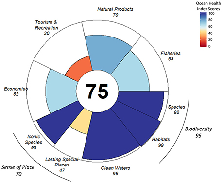
Figure 2. Ocean Health Index scores for the overall index (white center) and 7 goals (with the food provision goal only represented by the fisheries sub-goal, and the livelihoods and economies goal only represented by the economies sub-goal), and the sub-goals of biodiversity and sense of place, (petals with color ranging from red for low scores to blue for high scores). Scores for CCAMLR subareas are provided in Supplementary Materials.
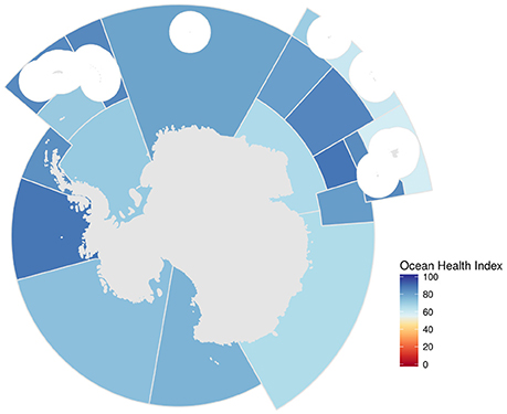
Figure 3. Map describing overall Ocean Health Index scores for CCAMLR areas. Scores can range from 0 (bad) to 100 (good). White circles are EEZ areas of island regions that were not included because they were analyzed in the Ocean Health Index global assessment.
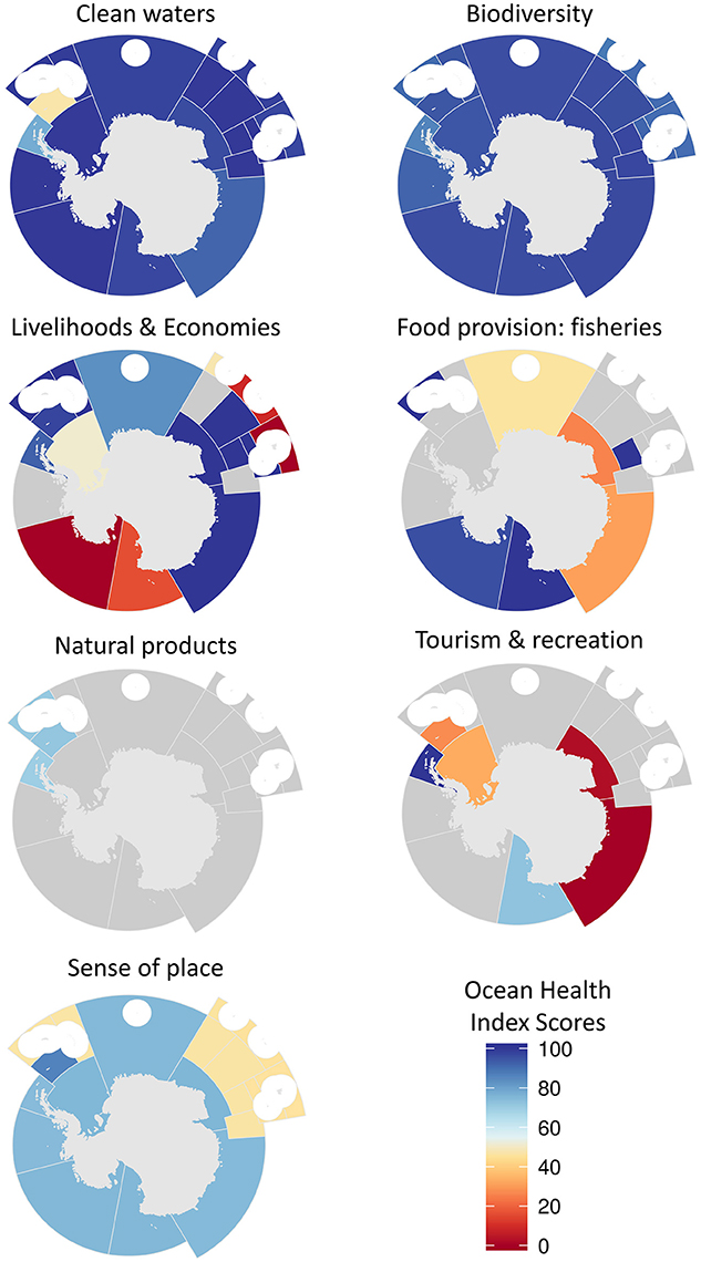
Figure 4. Maps of Ocean Health Index goal scores for CCAMLR areas. Scores range from 0 (bad) to 100 (good). Gray regions indicate the goal was not relevant to that area and thus not assessed. White circles are EEZ areas of island regions that were not included because they were analyzed in the Ocean Health Index global assessment.
The highest scoring goals/sub-goals, averaged across the Antarctic, were associated with conservation goals (Figure 2): clean waters (96) and biodiversity (96), with the habitat sub-goal within biodiversity scoring a near-perfect 99 and the species sub-goal 92. Sense of place (70) scored an intermediate value, reflecting a relatively low score for the lasting special places (47) sub-goal, whereas the iconic species (93) sub-goal achieved close to the highest score. Intermediate scores were also found for the two extraction-related goals: fisheries (63) and natural products (70). The final two goals were livelihoods & economies (62) and tourism and recreation (30), the lowest scoring goal for the Antarctic.
Clean waters scores were above 90 in all regions except for sub-region 48.1 (western Antarctic Peninsula) and 48.2 (Atlantic, south Scotia arc), scoring 78 and 47, respectively (Figure 4).
Biodiversity scores were relatively high within all regions (Figure 4). The species conservation sub-goal scored between 88 and 94 across sub-regions (Figure 5, Figures S2–S4), because most species are in the two lowest threat categories (i.e., near threatened and least concern, see Table S2). The habitat sub-goal scores, calculated using sea-ice season duration, were lower in regions near the Antarctic Peninsula, in particular along the western side of the peninsula (sub-region 48.1) (Figure 5, Figures S2–S4).
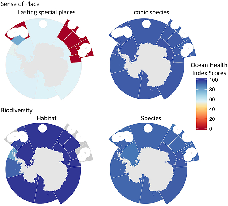
Figure 5. Maps of Ocean health Index scores for the sub-goals of biodiversity and lasting special places goals. Scores range from 0 (bad) to 100 (good). Gray regions indicate the goal was not relevant to that area and thus not assessed. White circles are EEZ areas of island regions that were not included because they were analyzed in the Ocean Health Index global assessment.
The results of testing an alternate version of the sea-ice indicator (Table S4) show some localized differences in scores around the Antarctic Peninsula and South Orkney Islands, namely for regions 48.1, 48.2, 48.4, and 88.1. These areas, would have lower biodiversity scores, with region 48.1, the Bellinghausen Sea, displaying the biggest difference of 20 points, changing from a score of 80 to 60. This modification of the model however would have a very small effect on the index calculated for the whole Antarctic region overall, i.e., a decline of just 1 point for the biodiversity score, and less than one for the overall index score.
Sense of place scores tended to be low in several regions (Figure 4), primarily because the lasting special places sub-goal received a score of 0 in several areas with no MPAs and no adjacent land (CCAMLR regions with coastal zones, received a score of 50, even with no MPAs because inland areas are considered protected; Figure 5, Figures S2–S4), and the highest score of 78 was obtained in region 48.2 (Bellinghausen Sea).
Fisheries data were present for only 7 regions (Figure 4, Figures S2–S4). Scores varied widely from 26 in 58.4.2 (western and central polar Indian Ocean adjacent to continent and including Prydz Bay) to 100 in the adjacent equatorward area 58.4.3a (central polar Indian Ocean).
The livelihood and economy goal scores (Figure 4, Figures S2–S4) ranged from 0 in region 88.2 (Amundsen Sea and eastern Ross Sea), and 9 in 58.6 (subpolar western Indian Ocean near Crozet Islands), to seven sub-regions that all scored 100 (48.3, 48.4, 58.4.1, 58.4.2, 58.4.3a, 58.4.b, and 58.5.2).
Natural products were only assessed in three sub-regions, 48.1-3 (western Antarctic Peninsula, South and North Scotia Arc), all with values close to 70 (Figure 4, Figures S2–S4).
Tourism (Figure 4, Figures S2–S4) scored well in areas 88.1 (western polar Pacific and Ross Sea) and 48.1 (western side of Antarctic Peninsula) (73 and 100, respectively), but scored very poorly in the other regions where it had been assessed (i.e., sub-regions 48.2, 48.5, and 58.4b in the Scotia Sea, Weddell Sea, and near Prydz Bay, respectively) (scores 27, 33, and 2, respectively).
Pressures mostly indicated very low stressor levels (scores closer to zero) (Figure 6), with sea-ice loss having a few higher values in 48.1 (western Antarctic Peninsula) and 48.2 (Bellinghausen Sea) due to declining ice-cover over time. Sea surface temperature showed some moderate pressure levels, mainly in the Southern Indian Ocean and Atlantic Ocean sides. Ocean acidification on the other hand showed unusually high values nearly everywhere, while pathogens reached a pressure value of 100 in the Southern Indian Ocean area.
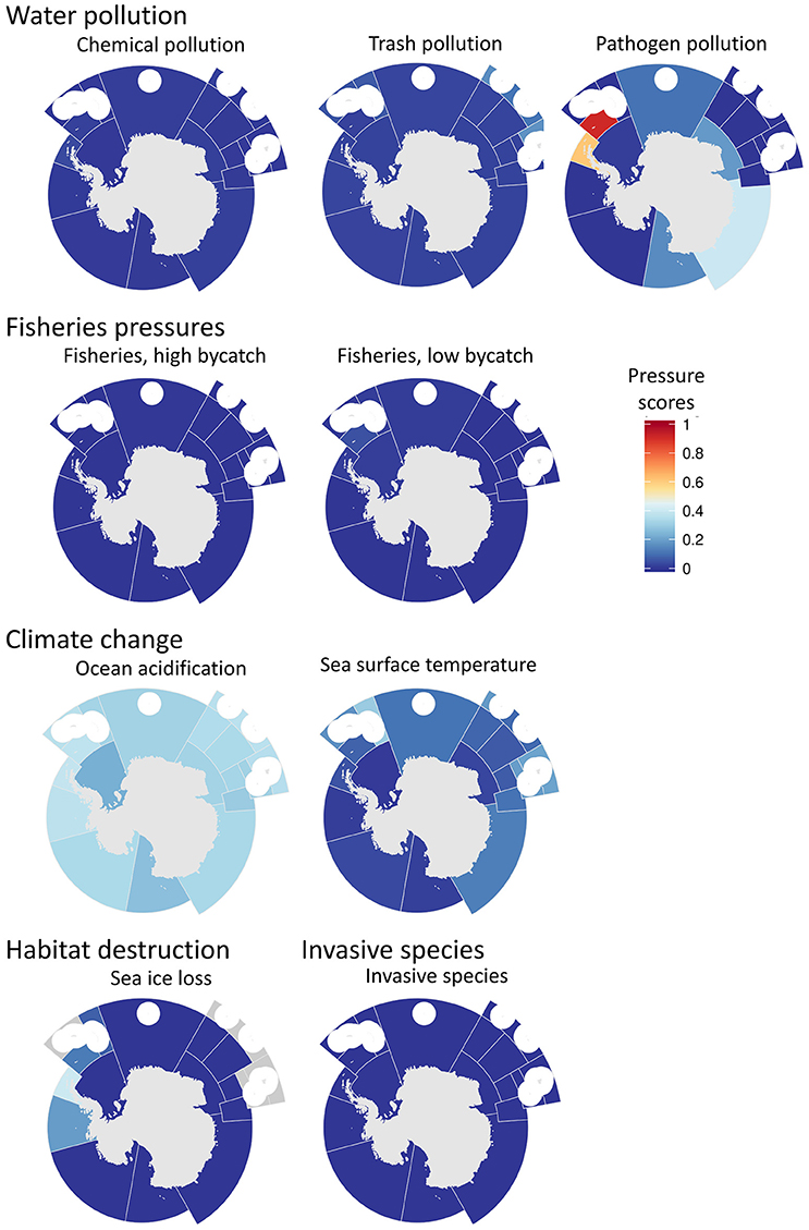
Figure 6. Maps of the pressure scores used in goal index score calculations, organized by pressure group (water pollution, fisheries pressures, climate change, habitat destruction, and invasive species). The pressure score describes the cumulative pressures acting on a goal, resulting in an expected decrease in the goal score. Note that the color ramping is reversed from other figures such that low (good) scores are blue and high (bad) scores are red. White circles are EEZ areas of island regions that were not included because they were analyzed in the Ocean Health Index global assessment.
Discussion
Understanding Scores in the Context of Antarctica
Biodiversity was the highest scoring goal, with the species sub-goal scoring well in part because of the successful rebuilding of once heavily exploited whale species (Leaper and Miller, 2011; Ainley and Pauly, 2014), seabird species as by-catch (Cox et al., 2007), and fur seals (Magera et al., 2013). However, of the species with known trends based on IUCN RedList assessments, 41 are stable or increasing while 38 are declining. There are 9 species that are endangered or critically endangered (baleen whales and an albatross species), and only one that is recovering (the blue whale), while the others are either declining or unknown. Moreover, of 132 species assessed, 53 have unknown trends. The knowledge gaps are also marked for iconic species, where 6 out of 38 species are data-deficient for their extinction risk and 19 have unknown population trends. Importantly, while the assessments produced by the International Union for Conservation of Nature (IUCN) and used here are representative of the entire species, regional studies, particularly those focusing on different penguin populations, suggest that the same species may respond differently in different parts of its distribution. For example, populations of the ice-obligate Adélie penguin have declined with time over much of the northern portion of the Western Antarctic Peninsula (48.1) but have been stable or grown further south along the Peninsula (Ducklow et al., 2007, 2013) and in the Ross Sea (88.1) (Lyver et al., 2014). This is explained, in part, by the different changes in sea-ice occurring simultaneously in different regions, although other factors such as food availability, ocean conditions, and weather conditions are also at play (Fraser et al., 2013).
The high habitat scores may be due to lack of sensitivity of the metric used to capture the health of sea-ice related ecosystems. First, ice season duration, as calculated from satellite images, captures the spatial and temporal extent of sea-ice coverage but does not account for sea-ice thickness, which may be critical to some organisms that use sea ice habitats (Stammerjohn et al., 2012). Second, accounting for changes in ice season across the vast spatial extent of the CCAMLR regions may smooth out higher resolution changes in sea ice, and fine-tuned phenology of organisms that adapted their life history to sea-ice season cycles (Stammerjohn et al., 2012). Third, although there has been notable sea-ice loss in the regions near the Antarctic Peninsula, both sea-ice extent and season duration has grown in many of the other regions of the Antarctic (Stammerjohn et al., 2008, 2012). Loss of sea ice as a critical habitat will have widespread effects throughout the Antarctic ecosystem, but the overall impact of increasing sea ice is less clear. It is possible that increasing sea-ice extent or season will have negative impacts on some species and positive impacts on others, as different penguin population trajectories seem to suggest (e.g., Dugger et al., 2014; Wilson et al., 2016). Thus, our treatment of the sea-ice status and pressure scores, negatively scoring only sea ice-loss, is likely a conservative estimate of the potential impact of habitat change on the Antarctic ecosystem as a whole.
The sensitivity test on the sea-ice reference point did show that, assuming a more rapid decline in biodiversity for habitats associated with sea-ice edge, would result in lower scores particularly in the regions around the Antarctic Peninsula and South Orkney Islands, particularly Bellinghausen Sea. However, this analysis didn't consider potential negative (or positive) effects of sea-ice extent increase. Importantly, we did not capture the impacts of increasingly unpredictable and variable annual sea-ice cycles on the phenology of species with very specialized life-history adaptations (Stammerjohn et al., 2012; Lyver et al., 2014).
The lasting special places goal scored relatively low due to the lack of Marine Protected Areas (MPAs) in the Southern Ocean (Brooks, 2013). Specifically, the only MPA large enough to have a notable effect on a sub-region's score is the South Orkney MPA (in sub-region 48.2). Other areas of special designation (Antarctic Specially Protected Areas, or ASPAs, and Antarctic Specially Managed Areas, or ASMAs), though valuable, had a relatively minor impact on OHI scores because of their extremely small spatial footprint.
The low food provision scores were due to catch levels below the maximum allowed, rather than unsustainable practices. The two stocks analyzed, Patagonian toothfish and Antarctic toothfish, are often well below their allowable catch, but in some cases they are shut down as fisheries when incidental (by-catch) species such as king crab, flying short-fin squid fisheries, lizardfish, sharks, and rays, and different species of bony fish reach their quotas. Any of the assessed by-catch species are managed based on very precautionary targets, rather than bioeconomic optimizations, and not marketable. Nevertheless, despite the fact that the management of fisheries in the Antarctic Treaty System area is regarded as better than most high-seas areas, challenges remain for enforcement and compliance in such a remote region (Österblom et al., 2014). Although Southern Ocean Illegal Unreported Unregulated fishing appears to have peaked in the late 1990s (Agnew et al., 2009), reports still indicate that IUU vessels are active, particularly in the Indian Ocean sectors (CCAMLR, 2014b). Enhanced satellite monitoring may help improve enforcement, i.e., through new software products that use vessel tracking data to infer the nature of vessel activity (e.g., such as Global Fishing Watch http://skytruth.org/2016/07/global-fishing-watch/). However, this would only be a partial solution as these products cannot provide proof, but only highlight potential problems that will need direct inspection to lead to prosecution. CCAMLR working groups try to use rough estimates of illegal catches to ensure toothfish catch quotas are robust to unreported harvests and are sufficiently precautionary, although these have not been officially reported since 2011, reportedly due to methodological issues (SC-CAMLR-XXIX, paragraph 6.5). Catches that are well below sustainable limits may be imposed in certain areas to take into account unreported removals by illegal fisheries (CCAMLR, 2014b).
The intermediate natural products scores reflect that harvested krill biomass is well below the current catch limits. In the three regions open to fishing, krill catch was 24, 12, and 12% of current precautionary catch limits in the 2014/2015 fishing season, leading to natural products scores of 70, 72, and 71 (Figure 4).
Tourism and recreation scored relatively poorly everywhere, except for the most visited region, the Antarctic Peninsula (sub-region 48.1). The sub-regions with low scores had declining local trends in visitors, which is not surprising, given the reduced overall number of tourists, likely due to recent global economic trends. It is worth noting that the same difficulties of enforcing rules as mentioned for fisheries regulations apply here. The establishment and enforcement of regulations restricting tourism currently rely largely on voluntary efforts on the part of tour operators themselves.
The revenues sub-goal, although measured with an imperfect proxy (i.e., changes in the number of crew on-board scientific or touristic vessels), was included to be able to explore potential tradeoffs or synergies with the other goals. The lowest scores were observed in the Ross Sea, the Weddell Sea, and a small region of the Indian Ocean close to Heard and MacDonald Islands. These spatial patterns in scores do not seem to match those observed for the food provision or tourism goals, although fishing and tourism are the activities used to measure it. Declines might reflect externally-driven increases in costs and/or declines in market demand rather than recent trends in fishing and tourism activity. This is coherent with the assumption that logistics and cost of fuel, rather than resource abundance, are the main constraints regulating the pursuit of commercial activities in the area.
The highest stressors were related to climate change and pathogens pressures (Figure 6). The strong presence of climate change impacts is expected, both because there are fewer opportunities for direct anthropogenic impacts and because of the greater exposure to elevated UV-radiation (high latitude and Antarctic Ozone Hole) and vulnerability to warming impacts (sea-ice is the main habitat we studied). Interestingly, the pressure from changing sea surface temperature was not consistent with the loss in sea-ice; rather, sea surface temperature pressures were higher in the Indian and Pacific regions around Antarctica.
Pressures from pollution were assessed using global models for chemical pollutants, nutrients and trash and local models for pathogen pollution, where the only major source of pathogens to Antarctic waters is from scientific research bases and ships (Tin et al., 2009; Martins et al., 2012; Corbett et al., 2014, 2015; Emnet et al., 2015). The volume of wastewater inputs and pathogen contamination in the Antarctic is small relative to many more populated coastal ocean regions. However, a more conservative reference point, taking into account sensitivity to small increments of pollutants, was used for the Antarctic compared to global assessments to capture the value placed on keeping Antarctica as pristine as possible. Consequently, relatively low clean water scores and high pathogen pressures were found for sub-regions with a large number of scientific research bases, even though the absolute amount of pollution was relatively small.
Finally, given the special conservation significance and existence value of the Antarctic to the global community, a more realistic overall ocean health assessment would require assigning different weights to the Ocean Health Index goals based on elicited values, which could lead to assigning higher weights to the scores for conservation-type goals (see Supplementary Materials). This would result in a higher overall score, as these are the goals that scored best. It would also be an incentive to focus governance efforts on maintaining these scores, or at the very least to carefully consider tradeoffs of enhancing other uses, such as increased harvests of krill and seafood and increased tourism.
Setting Reference Points in Antarctica
Some of the lower Ocean Health Index scores suggest an under-utilization of Antarctic resources. Although this might appear to suggest that the OHI score could be increased by intensifying extraction and use, intensified human activities are likely to increase the risk of pollution, pathogen contamination, and disturbance to wildlife, thus negatively affecting conservation-oriented goals such as clean waters and biodiversity conservation. In keeping with the principles that inspired the Antarctic Treaty, if Antarctica is to be preserved as a lasting special place that is valued by the international community for its existence value, it is reasonable to use conservative target values for human use and stressor intensity. Moreover, the Antarctic food web is likely more vulnerable and exposed to strong climate change impacts, both due to UV exposure and to the key importance of sea ice as a habitat, such that it may be prudent to adopt more conservative thresholds and reference points (Aronson et al., 2011).
We used the best available science to determine reference points, modifying them from those used in the global version of the Ocean Health Index (Halpern et al., 2015b). However, there were many challenges that arose due to limited or patchy data availability, in part because of the remoteness of the Antarctic region and limited observational coverage. This led us to develop region-specific reference points within the study area for many of the goals and pressures. Moreover, a poor understanding of the functional relationships between the indicators developed and the benefits they are meant to track, such as, for example, sea-ice habitat health, required making several simplifying assumptions in the analysis. Below, we describe the limitations of the data and reference points chosen for the various goals.
For fisheries, reference points were based on those set through formal species assessments. CCAMLR has made efforts to bring fisheries under stricter control by reducing harmful practices, for example by requiring changes to gear deployment methods to reduce bird bycatch, or by implementing move-on rules to avoid concentrating fishing effort on both target and by-catch species in one area (CCAMLR; https://www.ccamlr.org/en/compliance/compliance). CCAMLR is also inspecting landing ports in order to control illegally-caught toothfish, further incentivized by chain of custody certification programs such as the Marine Stewardship Council (Roheim and Sutinen, 2006) however, there are still several anecdotal sources reporting the presence of illegal unreported and unregulated fisheries (IUUs) in some of the areas (e.g., CCAMLR, 2014b). Illegal fishing can lead to underestimation of the actual overall level of harvest, can bias stock assessments, and increase the chance of overexploitation and stock collapse (Agnew et al., 2009). Although this may have, in part, affected our estimates, in order to reduce this risk, the CCAMLR working group on fish stock assessments (https://www.ccamlr.org/en/science/working-group-fish-stock-assessment-wg-fsa) attempts to estimate illegal harvest and incorporate it into the assessments used to determine legal catch quotas.
Regarding natural products, the krill fishery was one of the earliest fisheries to receive an ecosystem-based management target. This process allocates a sustainable harvest target after accounting for other predators' needs, and the under-exploitation of the krill fishery suggests that current predator populations have sustainable levels of krill biomass. The catch limit applies to large areas for which region-specific harvest control rules have not been set, and a precautionary harvest target that is much lower than what is assumed to be the Maximum Sustainable Yield was set, i.e., roughly 1% of assumed stock biomass, due to concerns of localized impacts on predators if fishing effort were to concentrate in small areas (Plagányi and Butterworth, 2012; Watters et al., 2013). Additional precaution might be warranted, though, given that the contemporary population abundances of predators (e.g., baleen whales) used to compute krill fishery catch limits may not properly take into account the ecological impact of historical overharvesting of marine mammals (e.g., Ainley et al., 2010; Surma et al., 2014). In other words, if the objective is rebuilding these predator populations to their pristine population abundances, it could result in lower krill biomass available for fishing than currently estimated, if predators' food requirements are to be fully taken into account (e.g., Ruzicka et al., 2013).
Because there were no data available on pathogen pollution to Antarctic waters, an Antarctic-specific pathogen model was chosen to highlight the impacts of untreated or partially-treated wastewater discharge. Reference points for this model were set based on research bases with the best possible wastewater treatment per annual average number of residents (see Supplementary Materials); however, more detailed data on the spatial extent of discharge impacts would increase this model's accuracy. For other contaminants, regionally-targeted models and reference points are needed for the Antarctic. Most pollution effects are likely too diluted, given the relatively small size of the sources and large area assessed in comparison to most other parts of the globe. If the pressure scores are calculated using the reference points adopted in the global Ocean Health Index, the Antarctic values are likely too small or too localized to greatly affect the index scores (Halpern et al., 2015a,b). Nonetheless, if these sources of contamination have influential local impacts, or are increasing, and the indicators are not sensitive enough to detect this change, this may be cause for concern and require finer-scale information so as to increase sensitivity.
Lacking any established benchmarks for tourism and recreation, we created a model based on best available knowledge. Most tour operators in the region belong to the International Association of Antarctic Tour Operators (IAATO). Although some guidelines for sustainable tourism are provided by the ATS, it is IAATO that established specific restrictions (e.g., no more than 500 tourists can land at a given site simultaneously; size limits on the boats allowed to approach land) that are enforced through self-regulation (Tin et al., 2009). Our assumption for using region specific reference points as a benchmark for tourism is that IAATO identified appropriate thresholds, and that most tour operators obey them. The highest observed density of visitors, by definition, would then be a sustainable amount. This approach also ensures that there is no penalty for avoiding places that are too arduous or distant to reach, and no incentive to visit pristine locations. The current method implies that, to improve health scores, tourism should be encouraged in accessible regions of Antarctica that at some point or other were visited by tourist cruises. However, sensitive regions may have already experienced negative impacts from too many tourist visitors (e.g., seabird rookeries, terrestrial vegetation, historical, and cultural artifacts; Tin et al., 2009), such that these past visitation rates are not appropriate reference values. In the future, the tourism and recreation goal should be reevaluated to consider possible mechanistic models for estimating the optimal amount of sustainable tourists, incorporating data on tourist disturbance rates and localized negative impacts into reference values.
Although the sensitivity test on the sea-ice habitat health reference point didn't produce a large difference on the overall index score, there were marked localized differences around the Antarctic Peninsula, which is also the area where most temperature warming has been observed in recent years. This exploration shows that important biodiversity threats may be currently overlooked due to the limitations of the information available. Importantly, it shows how the index can be used to explore the different assumptions that are made around reference points, exploring the range of possible values as different scenarios that could help highlight future risk. For example, different simulations on expected changes in sea-ice features could be used for the habitats indicator, as well as different assumptions about how this might impact biodiversity, by modifying the functional model used to calculate the goal status and trend.
Despite the creation of a whaling sanctuary in the Southern Ocean since 1994, Japan has continued harvesting minke whales (Balaenoptera bonaerensis), claiming a special permit due to scientific research purposes (see https://iwc.int/permits). In 2014 the International Court of Justice ruled that Japan's Special Permit programme in the Antarctic (known as JARPA II) did not meet special permit requirements (http://www.icj-cij.org/docket/index.php?p1=3&p2=3&k=64&case=148&code=aj&p3=4) and Japan ended it. The International Whaling Commission (IWC), responsible for overseeing the sanctuary's management, following the ruling, issued Resolution 2014-5 that calls for more thorough scientific justifications in granting future research permits. It is telling of the divided opinions within the Commission that it did not find consensus and had to be approved by majority vote (https://archive.iwc.int/pages/view.php?ref=3723&search=%21collection72&order_by=relevance&sort=DESC&offset=0&archive=0&k=&curpos=0). Since then, Japan has set out to capture 333 minke whale individuals in 2015, under a research plan purportedly meeting IWC requirements, but that instead raised new controversy (e.g., http://news.nationalgeographic.com/news/2014/09/140918-japan-scientific-whale-hunt-animals-ocean-science/).
Although the conservation status of minke whales is captured within the biodiversity and iconic species goal calculations, it would be possible to add a pressure layer that accounts for risks to the minke whale population due to harvest pressure. The lack of clarity and consensus over this type of issue on the part of the Whaling Commission may also be seen as a weakness in governance that would warrant assigning a lower biodiversity resilience score. Although it is an important issue to consider from both an ecological and a social perspective, such modifications would probably have a negligible effect on the overall scores of the region's health. We felt that these detailed modeling questions went beyond the scope of the current study, but could be addressed in future calculations of the index.
Governance and Long-Term Sustainability
Several countries have championed initiatives to designate large areas of the Southern Ocean as protected, but to date these efforts have systematically failed. At the time these analyses were performed, negotiations over a proposed system of protected zones championed by the US, New Zealand, and several NGOs in the Ross Sea were vetoed by Russia and the Ukraine, exposing vested interests in future resource extraction options (once the current moratorium is lifted in view of the 2048 review of the Antarctic Treaty System, or possibly earlier) (Brooks, 2013; Jacquet and Brooks, 2015). During the revision phase of the manuscript, thanks to Russia's change of position, this proposal was finally accepted during CCAMLR's 35th Annual meeting in Hobart (https://www.ccamlr.org/en/news/2016/ccamlr-create-worlds-largest-marine-protected-area). This can be seen as a sign of effectiveness of the ATS, as a multi-national governance system that can make important decisions, such as protecting an area as large as 1.55 Km2 of ocean, with unanimous agreement of its members. Nevertheless, the agreement was reached by changing the time frame of the Marine Protected Area from being in perpetuity, down to a time-bound limit of 35 years. Under these circumstances, whether this MPA could be included in the calculation of the sense of place goal, in the component valuing special places meant to be “lasting,” is up for debate. Moreover, the length of negotiations, the amount of stake-holder engagement required, and the fact that this represents one of the areas with more data and research (CCAMLR, 2014c), as this study also highlighted, suggest that adding more protected areas in the Southern Ocean in the future will not be a simple task.
A global region such as Antarctica that has been identified by the international community as a conservation priority, and that is especially fragile compared to other more resilient ecosystems (Aronson et al., 2011), should likely have more conservative benchmarks. For example, there is increasing evidence that tourists and scientists visiting Antarctica have been a source of invasive species, and climate change may open up a window for an accelerated rate of biological invasions (Frenot et al., 2005; Aronson et al., 2007; Shaw et al., 2014). These studies have mainly focused on terrestrial species that may be transported in the form of spores and pollen on clothing, but marine alien species may have gone undetected. Similarly, lack of good quality information on ship traffic may have led to underestimation of some types of chemical pollution and oil spills.
Importantly, there remains significant uncertainty in how climate change-driven stressors affect food-web dynamics, and therefore the delivery of many of the goals, largely due to insufficient spatial coverage of the data necessary to inform smaller scale assessments, and limitations in our knowledge of the function and dynamics of many socio-ecological processes in the region (Schofield et al., 2010; Kennicutt et al., 2014). For example, Barnes and Souster (2011) found significant impacts on benthic communities of climate-driven iceberg detachment, yet these types of interactions are not captured in our analysis. These uncertainties further challenge efforts to establish simple, reliable indicators to track change.
Summary and Conclusions
Antarctica is one of the most inaccessible parts of the world, but it is not pristine. Our analysis suggests that the Antarctic is not delivering benefits to people to its full potential. The analysis also highlights the measurable anthropogenic impacts and limitations in conservation measures in the area, despite best intentions to preserve its unique ecosystems and wildlife. As noted above, the value and quality of the current Antarctic OHI assessment is constrained by data and knowledge limitations, suggesting the need for expanded observational efforts and more mechanistic research on both natural and social science aspects of the Antarctic system. For example, the status of a number of Antarctic species is still unknown, and there is insufficient spatial coverage for key environmental factors to fully assess habitat and ecosystem health. Region-specific biological studies often report regional differences in the biological responses to climate change, ocean warming, sea-ice loss, and ocean acidification, and we have a limited capability, at present, to model, and predict impacts across trophic scales (Murphy et al., 2012).
Our assessment is not designed to measure long-term environmental risk and sustainability. Rather, it was created to capture current and impending stressors and elements of governance under “business as usual” conditions. For example, growing ecological pressures, such as climate change, and potential changes in political governance are not easily captured in the likely future state of the Index. We showed an example of how the OHI can be used to conduct explorations of areas of knowledge uncertainty, such as the relationship between sea-ice parameters and the preservation of associated biodiversity. Leveraging model-based climate simulations, projected future scenarios of index scores can be constructed as a useful companion analysis with the current index assessment framework to gain a longer-term vision of tradeoffs and risks, particularly given the influential role of climate change in determining the health of the region.
Progress in understanding and assessing Antarctic ecosystem health requires a deeper understanding of the complex physical and oceanographic dynamics (Kennicutt et al., 2014) and the many political decisions involving the region's governance (Gales et al., 2014). Both perspectives underscore the difficult challenges lying ahead for this unique system. The dispute over the institution of MPAs may be seen as a preview of the type of conflicts to come. Indeed, our study highlights the need for the international community to reconcile conservation versus utilitarian goals for Antarctica (Jacquet et al., 2016). Even with such understanding in place, a major challenge remains in enforcing compliance of existing or new rules over such a vast, remote, and environmentally harsh region. Maintaining and enhancing agreements among Antarctic Treaty signatories will be crucial to ensure long-term protection of local species and habitats. Moreover, given the importance of climate change-driven stressors, not all threats to the Antarctic can be addressed through local governance. Global climate change mitigation, which requires concerted international efforts to reduce greenhouse gas emissions, will play an increasingly crucial role in preserving the health of the Antarctic continent and Southern Ocean.
Author Contributions
BH and CL conceived of the project. CL, MF, SD, JR, and JM provided and processed data. MF, CL, SD, and JR conducted analyses. MF produced figures. BH, SD, CL, and MF drafted the paper. All authors revised the paper.
Funding
Beau and Heather Wrigley and the Pacific Life Foundation generously provided the founding support to the Ocean Health Index. Financial and in-kind support has also been provided by the Thomas W. Haas Fund of the New Hampshire Charitable Foundation, Jayne and Hans Huffschmid, Oak Foundation, Joseph S. and Diane H. Steinberg Charitable Trust, and the Akiko Shiraki Dynner Fund for Ocean Exploration and Conservation. SD and JR acknowledge support from the Palmer LTER program via funding from the National Science Foundation Polar Programs (NSF PLR-1440435).
Conflict of Interest Statement
The authors declare that the research was conducted in the absence of any commercial or financial relationships that could be construed as a potential conflict of interest.
Acknowledgments
Thanks to Sharon Stammerjohn, Elizabeth Selig, Trond Kristiansen, and Molly Troup for help providing data and advice on how best to use those data.
Supplementary Material
The Supplementary Material for this article can be found online at: https://www.frontiersin.org/article/10.3389/fmars.2017.00020/full#supplementary-material
References
Agnew, D. J., Pearce, J., Pramod, G., Peatman, T., Watson, R., Beddington, J. R., et al. (2009). Estimating the worldwide extent of illegal fishing. PLoS ONE 4:e4570. doi: 10.1371/journal.pone.0004570
Ainley, D. G., Ballard, G., Blight, L. K., Ackley, S., Emslie, S. D., Lescroel, A., et al. (2010). Impacts of cetaceans on the structure of Southern Ocean food webs. Mar. Mamm. Sci. 26, 482–498. doi: 10.1111/j.1748-7692.2009.00337.x
Ainley, D. G., and Pauly, D. (2014). Fishing down the food web of the Antarctic continental shelf and slope. Polar Record 50, 92–107. doi: 10.1017/S0032247412000757
Aronson, R. B., Thatje, S., Clarke, A., Peck, L. S., Blake, D. B., Wilga, C. D., et al. (2007). Climate change and invasibility of the Antarctic benthos. Ann. Rev. Ecol. Evol. Syst. 38, 129–154. doi: 10.1146/annurev.ecolsys.38.091206.095525
Aronson, R. B., Thatje, S., McClintock, J. B., and Hughes, K. A. (2011). Anthropogenic impacts on marine ecosystems in Antarctica. Ann. N.Y. Acad. Sci. 1223, 82–107. doi: 10.1111/j.1749-6632.2010.05926.x
Barnes, D. K. A., and Souster, T. (2011). Reduced survival of Antarctic benthos linked to climate-induced iceberg scouring. Nat. Clim. Change 1, 365–368. doi: 10.1038/nclimate1232
Brooks, C. M. (2013). Competing values on the Antarctic high seas: CCAMLR and the challenge of marine-protected areas. J. Polar Res. 2, 277–300. doi: 10.1080/2154896X.2013.854597
CCAMLR (2014a). CCAMLR Ecosystem Monitoring Program: Standard Methods. Available online at: www.ccamlr.org
CCAMLR (2014b). CCAMLR Fishery Report 2014: Closed Fishery for Dissostichus spp. in Divisions 58.4.4a and 58.4.4b. CCAMLR.
CCAMLR (2014c). Chronology of Previously Submitted Scientific Documents, and Updated Maps and Analyses Supporting MPA Planning in the ROSS SEA Region. SC-CCAMLR-XXXIII/BG/23 Rev.1. Agenda item No. 5.2. Available online at: https://www.mfat.govt.nz/assets/_securedfiles/Environment/Chronology-of-previously-submitted-scientific-documents-and-updated-maps-and-analyses-supporting-MPA-planning-in-the-Ross-Sea-region-September-2014.pdf
Chown, S. L., Clarke, A., Fraser, C. I., Craig Cary, S., Moon, K. L., and McGeoch, M. A. (2015). The changing form of Antarctic biodiversity. Nature 522, 431–438. doi: 10.1038/nature14505
Corbett, P. A., King, C., and Mondon, J. A. (2015). Tracking spatial distribution of human-derived wastewater from Davis Station, East Antarctica using δ15N and δ13C stable isotopes. Mar. Pollut. Bull. 90, 41–47. doi: 10.1016/j.marpolbul.2014.11.034
Corbett, P. A., King, C., Stark, J. S., and Mondon, J. A. (2014). Direct evidence of histopathological imapacts of wastewater discharge on resident Antarctic fish (Trematomus bernacchii) at Davis Station, East Antarctica. Mar. Pollut. Bull. 87, 48–56. doi: 10.1016/j.marpolbul.2014.08.012
Cox, T. M., Lewison, R. L., Zydelis, R., Crowder, L. B., Safina, C., and Read, A. J. (2007). Comparing effectiveness of experimental and implemented bycatch reduction measures: the ideal and the real. Conserv. Biol. 21, 1155–1164. doi: 10.1111/j.1523-1739.2007.00772.x
Doney, S. C., Bopp, L., and Long, M. C. (2014). Historical and future trends in ocean climate and biogeochemistry. Oceanography 27, 108–119. doi: 10.5670/oceanog.2014.14
Doney, S. C., Fabry, V. J., Feely, R. A., and Kleypas, J. A. (2009). Ocean acidification: the other CO2 problem. Annu. Rev. Mar. Sci. 1, 169–192. doi: 10.1146/annurev.marine.010908.163834
Doney, S. C., Ruckelshaus, M., Duffy, J. E., Barry, J. P., Chan, F., English, C. A., et al. (2012). Climate change impacts on marine ecosystems. Annu. Rev. Mar. Sci. 4, 11–37. doi: 10.1146/annurev-marine-041911-111611
Ducklow, H. W., Baker, K. S., Martinson, D. G., Quetin, L. B., Ross, R. M., Smith, R. C., et al. (2007). Marine pelagic ecosystems: the West Antarctic Peninsula. Philos. Trans. R. Soc. Lond. 362, 67–94. doi: 10.1098/rstb.2006.1955
Ducklow, H. W., Clarke, A., Dickhut, R., Doney, S. C., Geisz, H., Huang, K., et al. (2012). “The marine ecosystem of the West Antarctic Peninsula,” in Antarctica Ecosystems: An Extreme Environment in a Changing World, eds A. D. Rogers, N. M. Johnston, E. J. Murphy, and A. Clarke (Wiley-Blackwell), 121–159.
Ducklow, H. W., Fraser, W. R., Meredith, M. P., Stammerjohn, S. E., Doney, S. C., Martinson, D. G., et al. (2013). West Antarctic Peninsula: an ice-dependent coastal marine ecosystem in transition. Oceanography 26, 190–303. doi: 10.5670/oceanog.2013.62
Dugger, K. M., Ballard, B., Ainley, D. G., Lyver, P. O., and Schine, C. (2014). Adélie penguins coping with environmental change: results from a natural experiment at the edge of their breeding range. Front. Ecol. Evol. 2:68. doi: 10.3389/fevo.2014.00068
Emnet, P., Gaw, S., Northcott, G., Storey, B., and Graham, L. (2015). Personal care products and steroid hormones in the Antarctic coastal environment associated with two Antarctic research stations, McMurdo Station and Scott Base. Environ. Res. 136, 331–342. doi: 10.1016/j.envres.2014.10.019
Fraser, W., Patterson-Fraser, D., Ribic, C. A., Schofield, O., and Ducklow, H. (2013). A non-marine source of variability in adélie penguin demography. Oceanography 26, 207–209. doi: 10.5670/oceanog.2013.64
Frazier, M., Longo, C., and Halpern, B. S. (2016). Mapping uncertainty due to missing data in the global ocean health index. PLoS ONE 11:e0160377. doi: 10.1371/journal.pone.0160377
Frenot, Y., Chown, S. L., Whinam, J., Selkirk, P. M., Convey, P., Skotnicki, M., et al. (2005). Biological invasions in the Antarctic: extent, impacts and implications. Biol. Rev. 80, 45–72. doi: 10.1017/S1464793104006542
Gales, N., Trathan, P., and Worby, A. (2014). Environment: social change affects Antarctic priorities. Nature 513:487. doi: 10.1038/513487a
Gröndahl, F., Sidenmark, J., and Thomsen, A. (2009). Survey of waste water disposal practices at Antarctic research stations. Polar Res. 28, 298–306. doi: 10.1111/j.1751-8369.2008.00056.x
Halpern, B. S., Frazier, M., Potapenko, J., Casey, K. S., Koenig, K., Longo, C., et al. (2015a). Spatial and temporal changes in cumulative human impacts on the world's ocean. Nat. Commun. 6:7615. doi: 10.1038/ncomms8615
Halpern, B. S., Longo, C., Hardy, D., McLeod, K. L., Samhouri, J. F., Katona, S. K., et al. (2012). An index to assess the health and benefits of the global ocean. Nature 488, 615–620. doi: 10.1038/nature11397
Halpern, B. S., Longo, C., Lowndes, J. S. S., Best, B. D., Frazier, M., Katona, S. K., et al. (2015b). Patterns and emerging trends in global ocean health. PLoS ONE 10:e0117863. doi: 10.1371/journal.pone.0117863
Halpern, B. S., Walbridge, S., Selkoe, K. A., Kappel, C. V. Micheli, F., D'Agrosa, C., et al. (2008). A global map of human impact on marine ecosystems. Science 319, 948–952. doi: 10.1126/science.1149345
IUCN (2015). The IUCN Red List of Threatened Species. International Union for the Conservation of Nature. Available online at: http://www.iucnredlist.org
Jacquet, J., Blood-Patterson, E., Brooks, C., and Ainley, D. (2016). ‘Rational use’ in Antarctic waters. Mar. Policy 63, 28–34. doi: 10.1016/j.marpol.2015.09.031
Jacquet, J., and Brooks, C. (2015). Conservation: it is rational to protect Antarctica. Nature 528:39. doi: 10.1038/528039a
Kaschner, K., Rius-Barile, J., Kesner-Reyes, K., Garilao, C., Kullander, S., Rees, T., and Froese, R. (2015). AquaMaps: Predicted Range Maps for Aquatic Species. Available online at: www.aquamaps.org
Kennicutt, M. C., Chown, S. L., Cassano, J. J., Liggett, D., Massom, R., Peck, L. S., et al. (2014). Polar research: six priorities for Antarctic science. Nature 512, 23–25. doi: 10.1038/512023a
Khatiwala, S., Tanhua, T., Mikaloff Fletcher, S., Gerber, M., Doney, S. C., Graven, H. D., et al. (2013). Global ocean storage of anthropogenic carbon. Biogeosciences 10, 2169–2191. doi: 10.5194/bg-10-2169-2013
Leaper, R., and Miller, C. (2011). Management of Antarctic baleen whales amid past exploitation, current threats and complex marine ecosystems. Antarct. Sci. 23, 503–529. doi: 10.1017/S0954102011000708
Lowndes, J. S. S., Pacheco, E. J., Best, B. D., Scarborough, C., Longo, C., Katona, S. K., et al. (2015). Best practices for assessing ocean health in multiple contexts using tailorable frameworks. PeerJ 3:e1503. doi: 10.7717/peerj.1503
Lyver, P. O., Barron, M., Barton, K. J., Ainley, D. G., Pollard, A., Gordon, S., et al. (2014). Trends in the breeding population of Adélie Penguins in the Ross Sea, 1981–2012: A coincidence of climate and resource extraction effects. PLoS ONE 9:e91188. doi: 10.1371/journal.pone.0091188
Magera, A. M., Mills Flemming, J. E., Kaschner, K., Christensen, L. B., and Lotze, H. K. (2013). Recovery trends in marine mammal populations. PLoS ONE 8:e77908. doi: 10.1371/journal.pone.0077908
Martins, C. C., Aguiar, S. N., Bicego, C. M., and Montone, R. C. (2012). Sewage organic markers in surface sediments around the Brazilian Antarctic station: results from the 2009/10 austral summer and historical tendencies. Mar. Pollut. Bull. 64, 2867–2870. doi: 10.1016/j.marpolbul.2012.08.019
Molnar, J. L., Gamboa, R. L., Revenga, C., and Spalding, M. D. (2008). Assessing the global threat of invasive species to marine biodiversity. Front. Ecol. Environ. 6, 485–492. doi: 10.1890/070064
Murphy, E. J., Cavanagh, R. D., Hofmann, E. E., Hill, S. L., Constable, A. J., Costa, D. P., et al. (2012). Developing integrated models of Southern Ocean food webs: including ecological complexity, accounting for uncertainty and the importance of scale. Prog. Oceanogr. 102, 74–92. doi: 10.1016/j.pocean.2012.03.006
Österblom, H., Bodin, Ö., Rashid Sumaila, U., and Press, A. J. (2014). Reducing illegal fishing in the Southern Ocean: a global effort. Solut. J. 5, 72–79. Available online at: https://www.thesolutionsjournal.com/article/reducing-illegal-fishing-in-the-southern-ocean-a-global-effort/
Österblom, H., Sumaila, U. R., Bodin, Ö., Sundberg, J. H., and Press, A. J. (2010). Adapting to regional enforcement: fishing down the governance index. PLoS ONE 5:e12832. doi: 10.1371/journal.pone.0012832
Plagányi, E. E., and Butterworth, D. S. (2012). The Scotia Sea krill fishery and its possible impacts on dependent predators: modeling localized depletion of prey. Ecol. Appl. 22, 748–761. doi: 10.1890/11-0441.1
Roheim, C. A., and Sutinen, J. (2006). “Trade and marketplace measures to promote sustainable fishing practices,” in ICTSD Natural Resources, International Trade and Sustainable Development Series Issue Paper No. 3, International Centre for Trade and Sustainable Development and the High Seas Task Force. Geneva.
Ruzicka, J. J., Steele, J. H., Ballerini, T., Gaichas, S. K., and Ainley, D. G. (2013). Dividing up the pie: Whales, fish, and humans as competitors. Progr. Oceanogr. 116, 207–219. doi: 10.1016/j.pocean.2013.07.009
Samhouri, J. F., Lester, S. E., Selig, E. R., Halpern, B. S., Fogarty, M. J., Longo, C., et al. (2012). Sea sick? Setting targets to assess ocean health and ecosystem services. Ecosphere 3:41. doi: 10.1890/ES11-00366.1
Schofield, O., Ducklow, H. W., Martinson, D. G., Meredith, M. P., Moline, M. A., and Fraser, W. R. (2010). How do polar marine ecosystems respond to rapid climate change? Science 328, 1520–1523. doi: 10.1126/science.1185779
Shaw, J. D., Terauds, A., Riddle, M. J., Possingham, H. P., and Chown, S. L. (2014). Antarctica's protected areas are inadequate, unrepresentative, and at risk. PLoS Biol. 12:e1001888. doi: 10.1371/journal.pbio.1001888
Stammerjohn, S. E., Martinson, D. G., Smith, R. C., Yuan, X., and Rind, D. (2008). Trends in Antarctic annual sea ice retreat and advance and their relation to ENSO and southern annular mode variability. J. Geophys. Res. 113:C07004. doi: 10.1029/2007JC004269
Stammerjohn, S., Massom, R. A., Rind, D., and Martinson, D. (2012). Regions of rapid sea ice change: an inter-hemispheric seasonal comparison. Geophys. Res. Lett. 39:L06501. doi: 10.1029/2012gl050874
Surma, S., Pakhomov, E. A., and Pitcher, T. J. (2014). Effects of whaling on the structure of the southern ocean food web: insights on the “Krill Surplus” from Ecosystem Modelling. PLoS ONE 9:e114978. doi: 10.1371/journal.pone.0114978
Tin, T., Fleming, Z. L., Hughes, K. A., Ainley, D. G., Convey, P., Moreno, C. A., et al. (2009). Review: impacts of local human activities on the Antarctic environment. Antarct. Sci. 21, 3–33. doi: 10.1017/S0954102009001722
Watters, G. M., Hill, S. L., Hike, J. T., Matthews, J., and Reid, K. (2013). Decision-making for ecosystem-based management: evaluating options for a krill fishery with an ecosystem dynamics model. Ecol. Appl. 23, 710–725. doi: 10.1890/12-1371.1
Keywords: fisheries, polar, coupled systems, integrated assessment, Antarctic Treaty System
Citation: Longo CS, Frazier M, Doney SC, Rheuban JE, Humberstone JM and Halpern BS (2017) Using the Ocean Health Index to Identify Opportunities and Challenges to Improving Southern Ocean Ecosystem Health. Front. Mar. Sci. 4:20. doi: 10.3389/fmars.2017.00020
Received: 25 July 2016; Accepted: 16 January 2017;
Published: 03 February 2017.
Edited by:
Hervé Claustre, Centre National de la Recherche Scientifique, FranceReviewed by:
Frank Dehairs, Vrije Universiteit Brussel, BelgiumAlexandre Mignot, Massachusetts Institute of Technology, USA
Copyright © 2017 Longo, Frazier, Doney, Rheuban, Humberstone and Halpern. This is an open-access article distributed under the terms of the Creative Commons Attribution License (CC BY). The use, distribution or reproduction in other forums is permitted, provided the original author(s) or licensor are credited and that the original publication in this journal is cited, in accordance with accepted academic practice. No use, distribution or reproduction is permitted which does not comply with these terms.
*Correspondence: Benjamin S. Halpern, halpern@nceas.ucsb.edu