Air-Sea Fluxes With a Focus on Heat and Momentum
 Meghan F. Cronin1*
  Chelle L. Gentemann2
  James Edson3
  Iwao Ueki4
  Mark Bourassa5,6
  Shannon Brown7
  Carol Anne Clayson3
  Chris W. Fairall8
  J. Thomas Farrar3
  Sarah T. Gille9
  Sergey Gulev10
  Simon A. Josey11
  Seiji Kato12
  Masaki Katsumata4
  Elizabeth Kent11
  Marjolaine Krug13
  Peter J. Minnett14
  Rhys Parfitt5,6
  Rachel T. Pinker15
  Paul W. Stackhouse Jr.12
  Sebastiaan Swart16,17
  Hiroyuki Tomita18
  Douglas Vandemark19
  Robert A.Weller3
  Kunio Yoneyama4
  Lisan Yu3
  Dongxiao Zhang20
- 1Pacific Marine Environmental Laboratory, NOAA, Seattle, WA, United States
- 2Earth and Space Research, Seattle, WA, United States
- 3Woods Hole Oceanographic Institution, Woods Hole, MA, United States
- 4Japan Agency for Marine-Earth Science and Technology, Yokosuka, Japan
- 5Department of Earth, Ocean and Atmospheric Science, Florida State University, Tallahassee, FL, United States
- 6Center for Ocean-Atmospheric Prediction Studies (COAPS), Florida State University, Tallahassee, FL, United States
- 7Jet Propulsion Laboratory, California Institute of Technology, Pasadena, CA, United States
- 8Earth System Research Laboratory, NOAA, Boulder, CO, United States
- 9Scripps Institution of Oceanography, University of California, San Diego, La Jolla, CA, United States
- 10P.P.Shirshov Institute of Oceanology, Moscow, Russia
- 11National Oceanography Centre, Southampton, United Kingdom
- 12NASA Langley Research Center, Hampton, VA, United States
- 13Council for Scientific and Industrial Research, Cape Town, South Africa
- 14Rosensteil School of Marine and Atmospheric Science, University of Miami, Miami, FL, United States
- 15University of Maryland, College Park, College Park, MD, United States
- 16Department of Marine Sciences, University of Gothenburg, Gothenburg, Sweden
- 17Department of Oceanography, University of Cape Town, Rondebosch, South Africa
- 18Institute for Space-Earth Environmental Research, Nagoya University, Nagoya, Japan
- 19College of Engineering and Physical Sciences, University of New Hampshire, Durham, NH, United States
- 20Joint Institute for the Study of the Atmosphere and Ocean, University of Washington, Seattle, WA, United States
Turbulent and radiative exchanges of heat between the ocean and atmosphere (hereafter heat fluxes), ocean surface wind stress, and state variables used to estimate them, are Essential Ocean Variables (EOVs) and Essential Climate Variables (ECVs) influencing weather and climate. This paper describes an observational strategy for producing 3-hourly, 25-km (and an aspirational goal of hourly at 10-km) heat flux and wind stress fields over the global, ice-free ocean with breakthrough 1-day random uncertainty of 15 W m–2 and a bias of less than 5 W m–2. At present this accuracy target is met only for OceanSITES reference station moorings and research vessels (RVs) that follow best practices. To meet these targets globally, in the next decade, satellite-based observations must be optimized for boundary layer measurements of air temperature, humidity, sea surface temperature, and ocean wind stress. In order to tune and validate these satellite measurements, a complementary global in situ flux array, built around an expanded OceanSITES network of time series reference station moorings, is also needed. The array would include 500–1000 measurement platforms, including autonomous surface vehicles, moored and drifting buoys, RVs, the existing OceanSITES network of 22 flux sites, and new OceanSITES expanded in 19 key regions. This array would be globally distributed, with 1–3 measurement platforms in each nominal 10° by 10° box. These improved moisture and temperature profiles and surface data, if assimilated into Numerical Weather Prediction (NWP) models, would lead to better representation of cloud formation processes, improving state variables and surface radiative and turbulent fluxes from these models. The in situ flux array provides globally distributed measurements and metrics for satellite algorithm development, product validation, and for improving satellite-based, NWP and blended flux products. In addition, some of these flux platforms will also measure direct turbulent fluxes, which can be used to improve algorithms for computation of air-sea exchange of heat and momentum in flux products and models. With these improved air-sea fluxes, the ocean’s influence on the atmosphere will be better quantified and lead to improved long-term weather forecasts, seasonal-interannual-decadal climate predictions, and regional climate projections.
Introduction
Societal Importance of Air-Sea Fluxes
The oceans impact weather and climate by heating (and cooling) the lower atmosphere. In particular, as seawater evaporates, the ocean surface cools; and when the moisture later condenses into cloud droplets, this heat is released, warming the atmosphere. This moistening, and then warming, makes the air buoyant, driving low-level baroclinicity and atmospheric convection, causing wind convergence at the surface and divergence aloft. At the equator, ocean heating of the atmosphere can result in towering convective clouds that reach the top of the troposphere. These disturbances in turn drive teleconnections in the atmosphere, affecting weather and climate remotely. Most dramatically, every 2–7 years, zonal shifts in the surface heating patterns along the equatorial Pacific, associated with El Niño Southern Oscillation (ENSO), lead to climate extremes across the world. Patterns of surface heat fluxes (Figures 1, 2) also affect large-scale atmospheric circulation patterns, with deep convection over the thermal equator forming the upward branch of the “Hadley Cell” that drives trade winds. Westerly jet streams in both hemispheres are likewise associated with vertical-meridional cells in the midlatitude and high latitudes. Again, their rising branches and storm tracks are aligned with the surface heating of the atmosphere associated with warm ocean western boundary currents that extend into the midlatitude ocean basins (Figures 1, 2). These surface wind patterns, e.g., westerly winds at high latitudes and easterly trades in the tropics, in turn drive the ocean general circulation. Western boundary currents associated with the wind-forced subtropical ocean gyres are particularly important as they carry warm water poleward, helping to transfer heat from the tropics (where there is greater heating of the earth’s surface by solar radiation per area) to higher latitudes (where heat lost at the surface by latent and sensible heat flux and net infrared cooling is greater than that gained by solar radiation). As discussed in this paper, quantifying these air-sea fluxes, which represent the direct communication between the ocean and atmosphere, is challenging. Through the recommendations presented here, we believe that remaining large biases and uncertainties that result in differences in global fields (Figures 1C–F) could be reduced by up to an order of magnitude, enabling better resolution of phenomena on scales ranging from sub-diurnal and mesoscale to global and interannual.
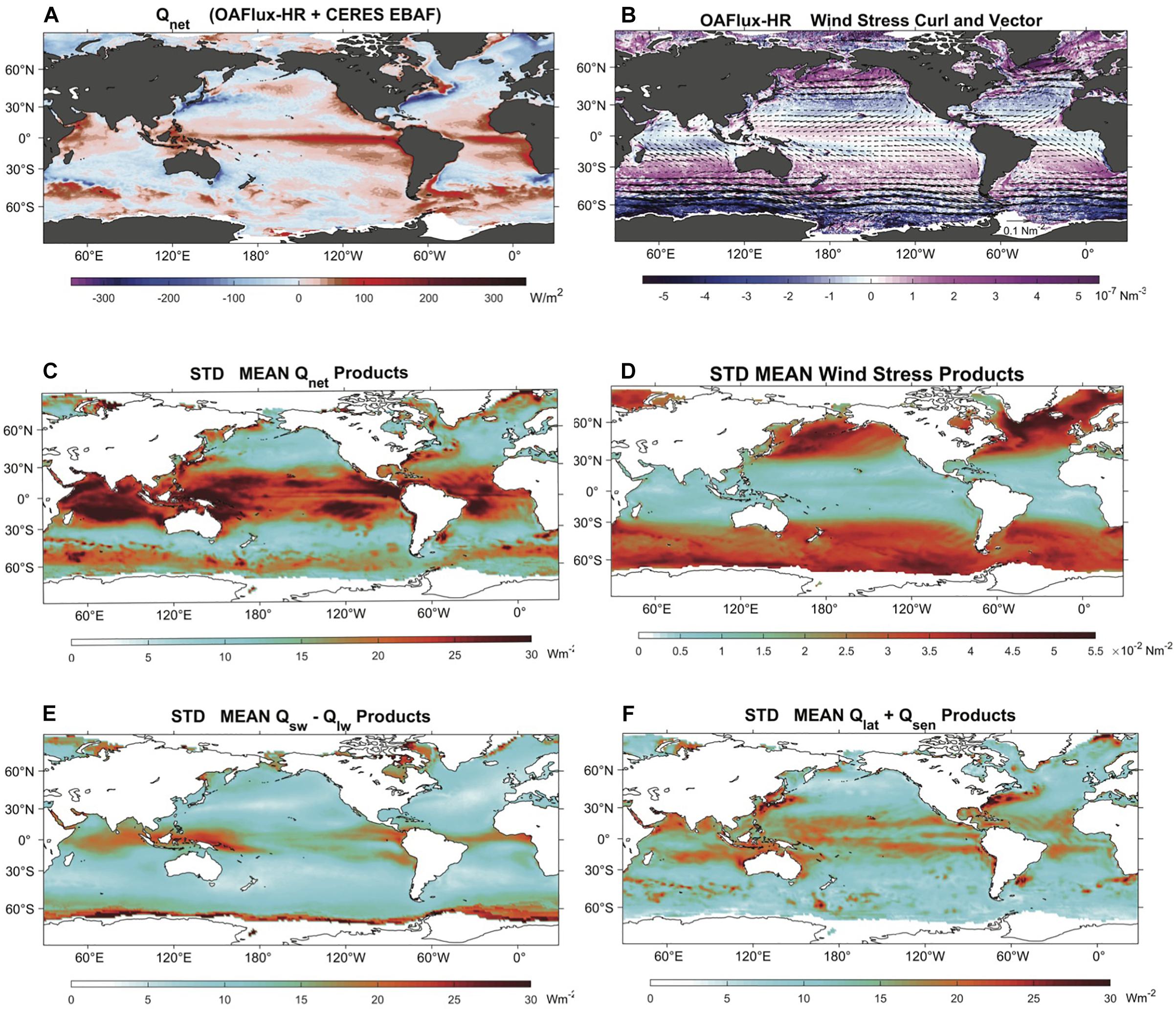
Figure 1. (A) Annual mean net surface heat flux (Qnet) for 2016 from the OAFlux-HR + CERES EBAFv4.0 product. (B) Annual mean wind stress curl and wind stress vectors for 2016 from the OAFlux-HR. (C) Standard deviation of annual-mean Qnet from 12 products. (D) Standard deviation of annual mean of surface wind stress magnitude from 12 products. (E) Standard deviation of annual-mean surface shortwave and longwave (Qsw – Qlw) from 10 products. (F) Standard deviation of annual-mean turbulent latent and sensible heat flux (Qlat + Qsen) from 11 products. Based on Yu (2019).
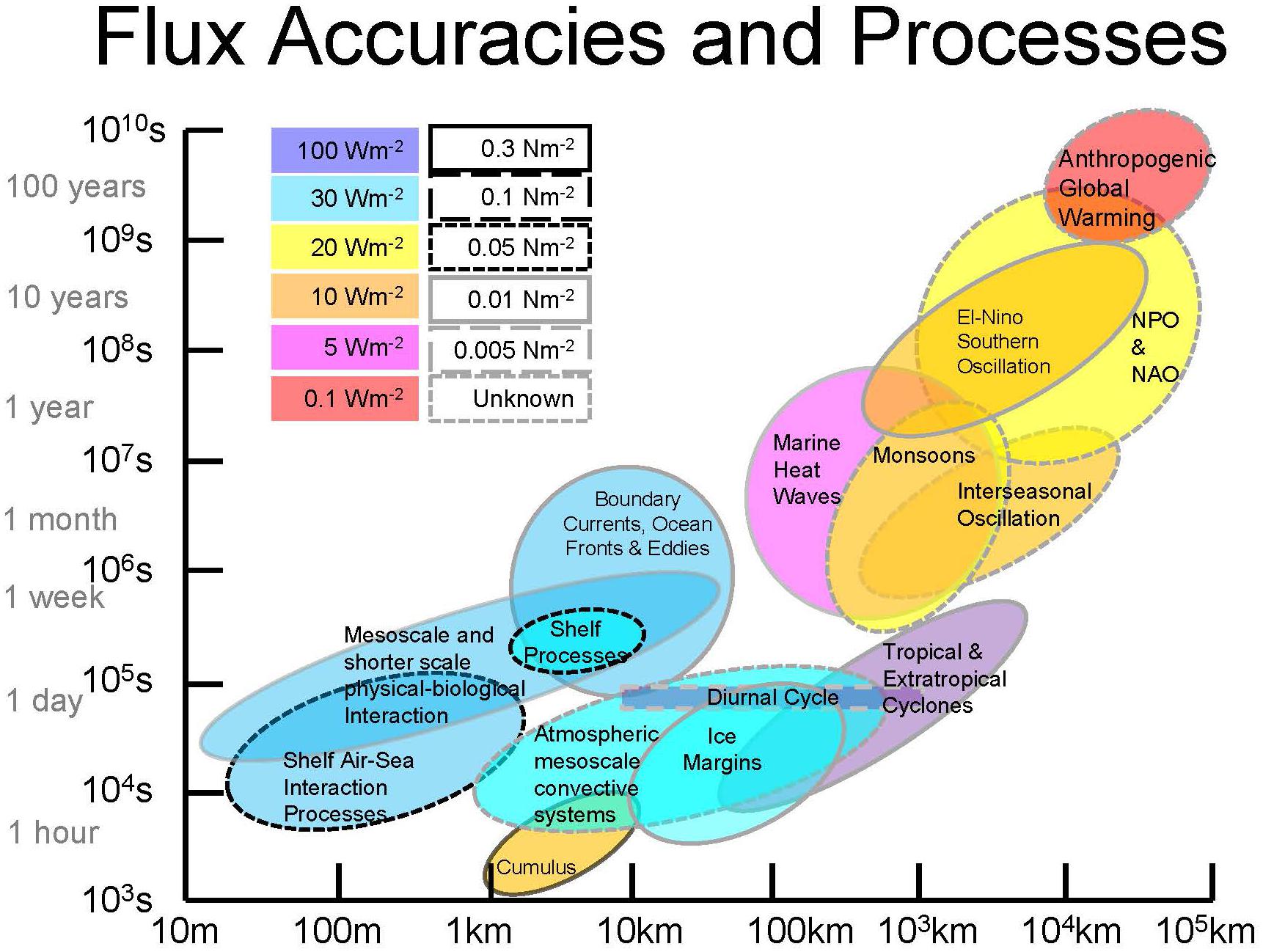
Figure 2. Target flux accuracy and scales for different phenomena. The space and time scales are indicated by the extent of the bubble. The target accuracies, estimated at 10 to 20% of the observed variability, are indicated by the color for net heat flux, and by the bubble’s outline for surface stress. The accuracy requirement for stress is a factor of 2 smaller for phenomena that are dependent on the curl of the stress rather than the stress magnitude. See Supplementary Table S1 for more detail. This figure is updated and adapted from Bourassa et al. (2013).
Reducing inaccuracies (both biases and random uncertainty) in air-sea fluxes is important for improving long-term weather and climate predictions. Because the ocean’s capacity to store heat is about 1000 times greater than that of the atmosphere, long-term weather and climate predictability has its origins in the oceans. Heat storage and release occurs on a range of time scales (Figure 2 and Supplementary Table S1) and can provide predictability out to 10–100 days (e.g., Madden-Julian Oscillation, Asian/Indian Monsoon), on seasonal-interannual time scales (e.g., ENSO), and out to decades (e.g., Pacific Decadal Oscillation, Atlantic Multidecadal Oscillation). Predictions of weather and climate on these time scales have great economic benefits for agriculture, water resource management, energy management, human and ecosystem health among others. Thus, to achieve useful predictions we must be able to quantify where, when and how much heat is released to the atmosphere. As a first step, here, we discuss strategies for improving our ability to quantify the amount of heat that at present is being exchanged between the ocean and atmosphere, regionally and globally. Because these air-sea heat exchanges are highly related to the surface dynamics and turbulent properties, we will also address quantification of wind stress.
Strong air-sea fluxes can occur on short time and space scales (Figure 2 and Supplementary Table S1), challenging both in situ (because of technical difficulties in extreme conditions and undersampling) and satellite observations (because of grid-averaging). The primary external time scales affecting air-sea fluxes are the diurnal cycle and the annual cycle associated orbital forcing. Internal dynamics lead to a range of other time and space scale variability in wind stress and air-sea heat fluxes. Sea-surface temperature (SST) fronts in the ocean are particularly critical to air-sea fluxes. The largest magnitude and temporal variability of air-sea fluxes is found in regions associated with SST fronts, specifically at western boundary currents such as the Gulf Stream, where intense poleward currents carry warm tropical water into the subtropics. In winter, large ocean heat loss is associated with cold air outbreaks, when cold and dry air blowing over much warmer water drive frequent episodic high flux events (e.g., Bond and Cronin, 2008; Shaman et al., 2010; Tilinina et al., 2018). Additionally, the intense SST gradients at ocean fronts result in strong heat flux gradients. These strong gradients in heat flux are known to be crucial for modulating both synoptic atmospheric variability and in turn the mean atmospheric state (Parfitt et al., 2016; Parfitt and Seo, 2018). Away from ocean fronts, whilst turbulent mixing of colder and dryer air aloft generally results in a near surface air temperature cooler than the SST and relative humidity less than 100%, the net surface heat loss from the ocean is much weaker. As will be discussed below, there are many challenges associated with resolving air-sea fluxes in regions of strong ocean fronts.
Because the specific heat capacity of water is considerably larger than that of land, air temperature is more variable over land than over the oceans, leading to a tendency for milder coastal climates than inland. Oceanic heat loss due to evaporation is associated with moisture fluxes that are an important source of water for agriculture and human consumption. Understanding and quantifying the exchange of heat and momentum between the ocean and atmosphere is therefore critically important for proper management of natural resources and reducing risks to vulnerable populations.
Quantifying Air-Sea Exchanges of Heat and Momentum
The net surface heat flux (Qnet) comprises net shortwave (i.e., solar) (QSW) and net longwave (i.e., infrared (IR) (QLW) radiative fluxes, and surface turbulent (latent and sensible) heat fluxes:
Surface latent heat flux, Qlat, is the heat extracted from the ocean when seawater evaporates. This heat is released to the atmosphere when and where this vapor condenses, forming clouds. Likewise, sensible heat flux, Qsen, is the heat extracted from the ocean associated with an air-sea temperature difference. The sign convention used here enables each term to be expressed generally as a positive value (i.e., as a magnitude) for most applications. When averaged over the global oceans and a full year, there should be a near-balance between solar radiative heating of the ocean (reduced by net longwave radiative heat loss), latent heat loss due to evaporation and sensible heat loss induced by air-sea temperature and humidity differences. However, due to biases in flux estimates, existing products have difficulties closing the heat budget, as discussed in section “Current Capabilities for Gridded Flux Products.”
The net shortwave radiation flux, QSW, is the net difference between the incoming (i.e., downwelling, SW ↓, and reflected outgoing shortwave radiations, SW ↑, and is commonly computed using a surface shortwave albedo, α = SW ↑ /SW ↓, estimate:
Likewise, because the outgoing surface longwave radiation LW ↑ comprises both the IR radiation emitted by the surface of the ocean and the portion of atmospheric downwelling IR radiation LW ↓ that is not absorbed by the ocean surface, the net longwave radiation flux, QLW, can be expressed as:
where ϵ is the IR surface emissivity (ϵ = 1 for black-body emission) and is taken to be equal to the absorptivity, σSB is Stefan-Boltzmann constant, and Ts is the surface (skin) temperature that is emitting the IR-radiation, in degrees Kelvin. The skin temperature of the ocean is generally cooler than the water beneath, as the ocean is nearly always and everywhere giving heat to the atmosphere (Fairall et al., 1996a). On the aqueous side of the interface, viscosity and the air-sea density difference prevent the turbulent transfer of heat from ocean to atmosphere and so the heat supplied to the interface to feed the latent and sensible heat fluxes and into the layer that emits infrared radiation to the atmosphere, is provided by molecular conduction, which requires a vertical temperature gradient. This temperature gradient is referred to as the thermal skin layer (Donlon et al., 2002; Minnett et al., 2011). As a result, the surface layer of the ocean is in nearly all cases cooler than at a depth of a millimeter or so. The thickness of the layer emitting infrared radiation that is subsequently measured by satellite radiometers to derive SST is comparable to the thermal skin layer (∼0.1 mm; Wong and Minnett, 2016, 2018), and so the derived temperature is referred to as the ocean skin temperature.
The latent and sensible heat fluxes are typically estimated from state variables, using a “bulk flux algorithm” (e.g., Fairall et al., 2003). As described in section “Turbulent Momentum and Heat Flux EOV and ECVs,” the primary state variables for turbulent fluxes, including wind stress, are surface winds relative to surface currents, skin temperature, near-surface air temperature, and near-surface humidity. Because most in situ estimates of the oceanic near-surface properties are below the skin, as discussed in section “Parameterizations to Extrapolate Measurements to Air-Sea Interface,” parameterizations must be used to extrapolate the bulk sea surface measurements to the air-sea interface. Likewise, as described in section “Parameterizations to Extrapolate Measurements to Air-Sea Interface,” flux EOV and ECV for the surface radiation include downward solar radiation, upward solar radiation (or surface albedo), downward longwave radiation, skin temperature, and longwave surface emissivity. We refer to the variables listed here as the “flux Essential Climate Variables (ECVs)” and “flux Essential Ocean Variables (EOVs).”
Turbulent Momentum and Heat Flux EOV and ECVs
The surface momentum (aka wind stress), sensible heat and latent heat fluxes provide surface boundary conditions for turbulent flux profiles in the lower atmosphere and upper ocean. These surface turbulent fluxes are most directly quantified by measuring the direct covariance (aka eddy correlation) between the fluctuating vertical velocity that drives the exchange with the fluctuating quantity of interest within the constant flux layer above the air-sea interface. For example, the directly measured latent heat flux is determined from
where ρ is the density of air; Lv is the latent heat of evaporation, w and q represent the fluctuating vertical velocity and specific humidity, respectively, and the brackets denote a temporal average of, generally, an hour or less. The turbulent fluxes, however, are difficult to measure at sea due to challenges that include platform motion contamination, flow distortion, high power requirements, rain and sea-spray contamination. Additionally, numerical forecast models do not resolve near surface turbulence, so surface fluxes must be parameterized.
These parameterizations are typically based on the assumption that the flux of some quantity is proportional to the vertical gradient of that quantity, e.g., the latent heat flux is proportional to the gradient in specific humidity. This approach, commonly referred to as the gradient or profile method, provides first-order closure in numerical models. The approach therefore requires vertical profiles of the observed or model-resolved non-turbulent state variables of temperature, specific humidity and velocity. The multiplicative factor that relates the flux to the gradient is known as the eddy viscosity for the momentum flux and the eddy diffusivity for the heat fluxes, e.g., the latent heat is determined from
where Kq is the eddy diffusivity for moisture, and ∂Q/∂z is the vertical gradient of the mean specific humidity. Commonly used parameterizations of the eddy viscosity and diffusivity in the surface (constant flux) layer assume that the efficiency of mixing by turbulent eddies scales with the height above the ocean surface. The efficiency of mixing is also a function of atmospheric stability, where mixing is suppressed under stable (thermally stratified) conditions and enhanced in unstable (convective) conditions. These two considerations predict semi-logarithmic profiles that includes a function that accounts for atmospheric stability.
It is also difficult, however, to measure vertical profiles and implement the gradient method over the ocean due to many of the challenges given for the direct covariance method. Instead, the surface fluxes are generally estimated using sea-air differences in the mean “bulk” state variables measured (or modeled) at the surface and at some height within the surface layer. The bulk aerodynamic method links the turbulent fluxes to mean air-sea velocity, temperature and humidity difference using transfer coefficients:
where cp is specific heat at constant pressure; u and v are the fluctuating along-wind and cross-wind velocity components, respectively; and θ is the fluctuating potential temperature; CD, CE, and CH are the transfer coefficients (known as the drag coefficient) for momentum, latent heat and sensible heat, respectively; S is the scalar wind speed relative to the ocean surface that includes gustiness; and ΔU, ΔV, ΔQ, and ΔΘ are the sea-air differences in the along-wind, crosswind, specific humidity and potential temperature, respectively.
At low winds, convective conditions, large-scale eddies drive gustiness that results in differences between the vector average wind components, U and V, and the wind speed, S, that includes gustiness. Convective gustiness has been shown to drive surface fluxes even when the vector-averaged winds are close to zero (Beljaars, 1995; Fairall et al., 1996b). However, the wind speed is difficult to measure on a moving platform due to wave contamination of the anemometers (i.e., vector averaging is used to remove this contamination but at the expense of gustiness). Additionally, the momentum equations in numerical models generally predict the vector components. Therefore, a common solution is to add convective gustiness to the vector averaged winds such that where Ug represents the gustiness due to convection. This is the approach used in the COARE algorithm (Fairall et al., 1996b). However, gustiness parameterizations that provide a single value of Ug regardless of height are physically inconsistent as convective gustiness is expected to vary with height within the boundary layer. More work is needed on this topic.
Although difficult, direct covariance estimates of the fluxes have been successfully measured from a variety of over-ocean platforms or a wide range of conditions as described in section “Current Capabilities.” These fluxes provide direct estimates of the transfer coefficients after normalization of the appropriate bulk state variables as given by Eq. 1.6. The measured transfer coefficients are then used to develop parameterizations of these coefficients that take into account two principal effects: atmospheric stability and ocean surface roughness. For example, direct measurements of the momentum flux are used to parameterize the drag as
where the middle term is the measured drag coefficient and the last term is a parameterization that includes a roughness length, z0, and a function that accounts for stability, ψu. This formulation is based on the assumption of a semi-logarithmic profile in the marine surface layer.
The impact of atmospheric stability is generally determined using Monin-Obukhov Similarity (MOS) scaling. MOS is used to develop functions (e.g., ψu) that account for the effects of stability in three overall stability classes: (1) neutral conditions, (2) unstable or convective conditions, and (3) stable or stratified conditions. Neutral surface layers are associated with high winds and little solar heating where turbulent mixing is driven by wind shear. The stability function equals zero under neutral conditions, i.e., ψu(neural) = 0, in the absence of convection or stratification. Unstable surface layers range from situations where turbulent mixing is completely driven by convective processes (aka free convection) to more common situations where the mixing is driven by both buoyancy and wind shear (aka forced convection). Stable surface layers force the wind shear to do work against the stratification, thereby inhibiting mixing and turbulent exchange.
While the form of the stability functions can be guided by scaling arguments (e.g., in the free convective limit), the actual form of these functions must be determined empirically from direct measurements. Successful formulations are able to parameterize the entire range of stability classes. Reasonably consistent formulations have been determined through observations in a number of overland (e.g., Dyer and Hicks, 1970; Businger et al., 1971; Dyer and Bradley, 1982), over-ice (e.g., Grachev et al., 2007) and overwater (e.g., Edson and Fairall, 1998; Vickers and Mahrt, 1999; Edson et al., 2004, 2007, 2013) investigations, which have shown MOS scaling to be valid as long as the assumptions central to its application are not violated. These include a constant turbulent flux layer, stationarity and horizontal homogeneity.
Before developing parameterizations that account for the varying roughness of the underlying sea surface, the impact of atmospheric stability must first be removed (e.g., Fairall et al., 1996b). This is done using the MOS stability functions by adjusting the transfer coefficients to neutral conditions where, e.g., ψu(0) = 0 and the neutral drag coefficient is defined as CDN = (ln(z/z0))2. The roughness length is commonly parameterized using the roughness Reynolds number for smooth flow to provide the surface “roughness” at low winds (Smith, 1988). Other low wind studies have suggested the use of Weber number scaling to parameterize the roughness as a function of surface tension (Wu, 1994). The low-wind roughness is added to another roughness length that accounts for the increasing roughness of surface waves at increasingly higher wind speeds. This roughness length commonly relies on a relationship suggested by Charnock (1955). The Charnock relationship effectively models the surface roughness due to wind-waves as the ratio of surface forcing (i.e., the surface stress) to the restoring force of gravity. This ratio is multiplied by a variable of proportionality known as the Charnock parameter.
The Charnock parameter is expected to account for the wide-range of physical processes that impact wind-wave interaction. Therefore, it should come as no surprise that there is a wide range of published parameterizations of the Charnock parameter. The transfer coefficients are known to have a wind speed dependence – strong for CD and weak for CE and CH. This dependence has naturally led to the parameterization of the transfer coefficients as a function of wind speed (e.g., Large and Pond, 1981) or using a wind-speed dependent Charnock parameter (e.g., Fairall et al., 2003). Other bulk algorithms have explicit dependencies on sea state (e.g., significant wave height, wave period and wave steepness, wave-age, directional differences between the wind and wave fields), and fraction of ice cover. Such dependencies in measured fluxes are often modeled using Charnock’s relationship where the Charnock parameter is parameterized in terms of the wind-speed, wave-slope, wave-age and ice fraction. However, understanding the relation between the roughness parameter and the sea state, and likewise the effect of sea state on the relative winds, remains an area of active research (e.g., Liu et al., 1979; Large and Pond, 1981; Donelan et al., 1993; Fairall et al., 1996b, 2003; Mahrt et al., 1996; Bourassa et al., 1999; Brunke et al., 2003; Drennan et al., 2005; Edson et al., 2013; Hristov and Ruiz-Plancarte, 2014).
The impact of waves on air sea-fluxes also extends to the sensible and latent heat fluxes. For example, many formulations of the transfer coefficients for sensible and latent heat include the drag coefficient to the one-half, , times a scalar component for heat and moisture; e.g., the transfer coefficient for latent heat can be defined as where Cq is the scalar component of the moisture transfer. This formulation predicts that any wave-related dependencies in the drag coefficient will be included in these formulations in a somewhat muted form. Analogous to the aerodynamic roughness length used to define the drag coefficient, the scalar components are commonly defined using “thermal” roughness lengths. For example, the transfer coefficient for latent heat has been defined as
where z0q is the thermal roughness length for moisture and ψq is a MOS stability function for humidity. The thermal roughness lengths are often parameterized as a function of the roughness Reynolds number, which is defined using the aerodynamic roughness length (see Liu et al., 1979; Fairall et al., 1996b for details). As such, any wave-related parameterization of the aerodynamic roughness length will also be included in the thermal roughness lengths.
The more sophisticated algorithms account for the difference between a bulk water temperature and the interface temperature, wind gustiness, and surface currents, as discussed in section “Parameterizations to Extrapolate Measurements to Air-Sea Interface.” However, there is a balance between increasing parameterization complexity and hence dependence on additional variables that may be uncertain or unknown, and improvements that may be gained by considering additional physics. The COARE algorithm transfer coefficients are claimed to be accurate on average to approximately ± 5% for CD and CE (set equal to CH) for wind speeds from 2 to 20 m s–1. By this we mean that some 15,000 h of direct flux measurements, converted to transfer coefficients, and averaged in wind speed bins will be within 5% of the COARE transfer coefficients at the same wind speed. The scatter of individual 1-h measured values is about 25% and are generally wind speed and certainly platform dependent. This scatter is principally sampling error and is well-understood in terms of turbulence statistical theory (Blomquist et al., 2014). Research challenges that could lead to improved bulk flux parameterizations include:
• Development of wave-dependent surface flux parameterization that outperform wind-speed dependent parameterizations under a wide range of wind, wave and current conditions.
• Development of flux-profile relationships that account for both stratification and wave-induced perturbations on the wind profile though the wave boundary layer (WBL) and beyond under a wide range of wind, wave and current conditions.
• Development of surface flux and flux-profile relationships that account for directional differences between the wind and wave fields.
• Development of Geophysical Model Functions (GMF) to provide remotely sensed surface stress estimates that match or exceed the accuracy of bulk fluxes using in situ measurements.
• Development of convective gustiness parameterizations that are valid through the surface layer to the lowest grid point in high resolution forecast models.
• Development of gustiness parameterizations for coherent structures such as roll vortices in forced convection.
• Validation and continued development of models to simulate evaporating sea-spray and their impact on momentum, heat and mass fluxes under high to extreme wind conditions.
• Development of scale-dependent flux parameterizations for nested high-resolution models down to Large Eddy Simulation (LES) scale.
• Development of coupled LES with sufficient accuracy to simulate wind-wave-current interaction near the ocean surface to provide output that can be considered data for parameterization and model development.
In summary, modern bulk algorithms need to better incorporate the impact of waves and currents on the magnitude and direction of the surface stress and their modulation of fluxes and mean profiles (e.g., Grachev et al., 2003; Hara and Belcher, 2004; Grare et al., 2013, 2018; Hristov and Ruiz-Plancarte, 2014; Buckley and Veron, 2016; Cifuentes-Lorenzen et al., 2018). The wavy boundary layer and shallow atmospheric boundary layers provide a number of additional challenges associated with sea-spray, gustiness, severe stratification and extreme winds. The impact of boundary layer processes on surface fluxes above the surface layer are best studied with additional boundary layer measurement in combination with numerical models and simulations. Therefore, resolving the main issues with bulk algorithms will require a combination of field observations and specialized atmosphere-wave models. Because of the many dependencies, detailed research models such as advanced wave codes (e.g., Kukulka et al., 2007; Banner and Morison, 2010; Kudryavtsev et al., 2014) and wave-LES models (e.g., Sullivan et al., 2014, 2018; Hara and Sullivan, 2015), in combination with observations in many different regimes, can provide a rational way to explore the phase space of parameterization variables.
Parameterizations to Extrapolate Measurements to Air-Sea Interface
While the transfer coefficients used in bulk algorithm introduce some uncertainty into the estimation of the surface air-sea fluxes, perhaps a larger uncertainty comes from treatment of the flux state variables used to estimate the flux. In particular, for most state-of-the-art bulk algorithms, the sea surface temperature (SST) and specific humidity are assumed to be ocean skin values. If instead, a bulk sea temperature is used (i.e., sea temperature measured at depths ranging between 0.01 and 5 m or even deeper), then it should be adjusted to the surface using either parameterizations or models. Fairall et al. (1996a), for example, uses first estimates of the net surface heat flux and wind stress to force a one-dimensional mixed-layer model of the diurnal warm layer relative to the pre-dawn conditions. This is then used to account for stratification (i.e., the warm layer) above the depth of the bulk temperature measurement. Fairall et al. (1996a) also provides a “cool skin” model to account for the surface cooling from non-solar radiative components of the net surface heat flux to compute the SST or skin temperature. Other methods exist for making these extrapolations. For example, the Webster et al. (1996) method relies upon a specification of wind speed and peak solar flux to compute the diurnal warm SST variability at the surface. Parameterizations in terms of wind speed lead to a simple thermal skin effect correction (Donlon et al., 2002; Minnett et al., 2011). For tropical open ocean environments, the average warm layer correction leads to about a 5 W m–2 increase in Qnet, while the average cool skin adjustment is a decrease of about 10 W m–2. However, corrections due to the warm layer can lead to substantially larger fluxes when the measurements are made at depth in the presence of large diurnal warming events.
Likewise, for these state-of-the-art bulk algorithms, surface current estimates are needed to compute the wind speed and vertical wind shear relative to ocean surface as given by ΔU and ΔV in Eq. 1.6. The resulting changes in stress are usually small compared to the stress except in regions of strong currents such as over western boundary currents. However, ignoring surface currents in the development of flux parameterization can lead to a systematic bias in the transfer coefficients (Edson et al., 2013) as the wind- and wave-driven currents are generally in the direction of the wind. As a result, the wind speed relative to water is generally smaller than the wind speed relative to earth. These differences are also large enough to cause substantial errors in the horizontal gradient of stress, which can have substantial impact on ocean circulation, upwelling, biology and biogeochemistry (Shi, 2017). Surface currents, however, are generally measured in situ at 10 m or deeper. There is growing appreciation that there can be non-negligible shear within the upper 10 m on timescales of the flux calculations. This can add to the errors in the relative wind, and potentially to errors in the flux parameterizations if the currents are not consistently adjusted to the surface. Brodeau et al. (2017) estimated the effect of surface currents on the wind stress to be on average within ± 0.005 N m–2 with the largest uncertainties amounting to 0.02–0.025 ± 0.005 N m–2.
Radiative Heat Flux EOV/ECV
The net radiative component of the air-sea heat flux comprises a shortwave component that is emitted by the sun (SW↓) and reflected from the ocean surface (SW↑) in the spectral range of 0.3–4.0 μm, and a longwave component that is emitted by the atmosphere (LW↓) and surface (LW↑) in the spectral range of 4.0–100.0 μm (Eqs 1.1–1.3). SW↓ has a direct and a diffuse component that interacts differently with the underlying surface due to differences in their spectral composition and angularly dependent properties. About half of the solar radiation incident on the top of the atmosphere reaches the surface of the Earth after being transmitted through the atmosphere. Extinction of solar radiation in the atmosphere is mostly by ozone, water vapor, clouds, and aerosols. The vertical profiles of clouds, water vapor, and temperature largely determine the longwave emission by the atmosphere. Clouds play a major role in determining the net radiative balance at the surface, dependent on their amount and optical properties (e.g., optical depth, a general measure of the capacity of a cloud to control the amount of light that will reach the surface). Most atmospheric constituents (e.g., cloud, aerosols, and water vapor) can now be derived from satellite instruments. At the ground, SW↓ is measured with pyranometers (spectral range of 0.310 to 2.800 μm) and LW↓ is measured with pyrgeometers (spectral range of 4.5 to 42 μm). The upward component of the surface solar radiation, SW↑, depends upon SW↓ spectral composition controlled by the solar zenith angle, atmospheric and cloud properties, as well as the surface optical properties, which depend upon the sea state (i.e., wind speed) and chlorophyll concentration in the upper ocean (Jin et al., 2004). In situ measurements of SW↑ are very rare and thus it is typically estimated from the SW↓ and surface albedo, α (Eq. 1.2).
The strong albedo dependence upon solar zenith angle means that more reflection occurs at lower sun angles (during dawn and dusk, in winter and at higher latitudes). Payne (1972) used observations of both upwelling and downwelling shortwave radiation to develop a relation between albedo and solar zenith angle and atmospheric transmittance. At low solar zenith angles, the albedo is 0.03 to 0.06, but at high solar zenith angles it can approach 0.3. Li et al. (2006) examined wind speed and zenith angle dependent models of the albedo from the perspective of upwelling shortwave at the top of the atmosphere. They found that differences among models were less than 10 W m–2 and the difference in the global mean was within ± 2.5 W m–2 compared with Clouds and the Earth’s Radiant Energy System (CERES) data. In the TOGA COARE bulk formulae, Fairall et al. (1996a) use a fixed albedo of 0.055. Errors in albedo can introduce errors in the net shortwave radiation and air-sea heat flux. Further work is needed to improve albedo parameterizations for use in state of the art bulk algorithms, Numerical Weather Prediction (NWP), and satellite radiation algorithms.
In situ observations of longwave radiation at sea have become more common only in the last 10–20 years. Prior to that, various bulk formulae for net longwave radiation at the sea surface were used that depended upon air- and sea-surface temperature, humidity, cloud cover (and type), and latitude (Fung et al., 1984). While in situ observations are used for local radiation budgets and for validations of computed radiative fluxes, only satellite observations can provide surface radiative fluxes at a global scale. To estimate radiative fluxes from satellite observations, we need to rely on radiative transfer models. Inputs for radiative transfer models include temperature and water vapor specific humidity vertical profiles, and cloud and aerosol properties. The accuracy of these properties largely influences the accuracy of surface radiative flux computations. Surface radiative fluxes are especially sensitive to near surface temperature and humidity profiles and boundary layer cloud properties. Consequently, improvements to these near surface properties are critical for reducing uncertainty in satellite-derived surface radiative fluxes.
Current Capabilities
Quantifying the air-sea fluxes over the global ice-free oceans requires a hierarchy of observations specifically targeted for (1) improving understanding of processes controlling air-sea exchange and their relationship to atmospheric and oceanic state variables, and specifically, for improving the “bulk algorithm” for computing these fluxes; (2) measuring flux EOVs and ECVs over the global ice-free ocean with sufficiently high spatial and temporal resolution, coverage, and accuracy to generate the global flux products; and (3) obtaining high-quality long time series and regionally distributed measurements that can be used for validating and improving these flux products. Here we describe the current capabilities of the in situ networks for measuring air-sea heat and momentum fluxes, and remotely sensed capabilities. Each has its strengths and weaknesses and NWP models are commonly used to integrate these disparate observations into dynamically consistent fields. We thus also describe current capabilities in NWP and hybrid NWP flux products.
Current Capabilities for in situ Flux EOV/ECV Measurements
ICOADS
The International Comprehensive Ocean-Atmosphere Data Set (ICOADS, Freeman et al., 2017, 2019) collates surface marine data extending back three centuries. Before about 1970 almost all ICOADS observations are from ship voyages but as ocean technology has developed, data from more platforms (surface moorings, drifters, floats) have been incorporated into the archive. At present, nearly all near-real time surface marine data available through the Global Telecommunication System (GTS) are incorporated into the database and periodically data from delayed mode archives are incorporated. Flux ECV and EOVs available through ICOADS include: SST, air temperature, humidity, wind speed and direction, barometric pressure, visually observed characteristics of sea state, and coded weather information. ICOADS contains few radiation measurements, but does contain visually observed cloud observations (Eastman et al., 2011). Sampling in ICOADS is very heterogeneous with observations concentrated in the major shipping routes of the Northern Hemisphere. Sampling errors in surface turbulent fluxes computed from ICOADS reports may amount to more than 60 W m–2 in poorly sampled regions (e.g., Gulev et al., 2007). ICOADS observations can be challenging to use, but if handled with care, ICOADS provides data for in situ flux calculations and global surface flux products (Josey et al., 1999; Berry and Kent, 2009). ICOADS also provides a major input data source for reanalyses (e.g., ERA-Interim: Dee et al., 2011; 20th Century Reanalysis: Compo et al., 2011; and CFSR: Saha et al., 2010). ICOADS is also the main in situ data source for the construction of gridded analyses of surface marine ECVs and EOVs including those used as surface boundary conditions for atmospheric reanalyses (e.g., HadSST3: Kennedy et al., 2011; ERSSTv5: Huang et al., 2017; COBE-SST2: Hirahara et al., 2014; HadNMAT2: Kent et al., 2013). Additionally, ICOADS data are used for satellite data calibration and evaluation (e.g., Jackson and Wick, 2010; Liman et al., 2018; Tomita et al., 2018), as well as long-term regional reconstructions of surface fluxes (Gulev et al., 2013). ICOADS is an archive for observations but requires access to expertly managed data from each different network type. Presently there is no international system for the expert management and archival of surface meteorological observations from the GTS although several national weather services maintain their own collections.
In situ Sensors for Measuring Fluxes
A typical set up to estimate the momentum, sensible heat and latent heat flux on a moving platform includes a 3-axis sonic anemometer/thermometer; a 3-axis motion package and an open path infrared hygrometer. Sonic anemometers/thermometers have become the tool of choice for marine research. Although they experience some dropouts and occasional spikes, particularly in rain, they are generally very reliable in the marine environment. Motion sensors are finding their way into many (non-marine) applications. As a result, researchers now have a number of small, low-power, reasonably inexpensive and sufficiently accurate motion packages to choose from. The infrared hygrometer is ideally deployed alongside a system that flushes the optics between rain events. A closed-path hygrometer avoids many issues associated with contamination of the optics. However, experience has shown that they suffer from uncorrectable attenuation of the signal due to the sticky nature of water vapor within sampling tubes in high humidity environments. The fluxes should be measured using the wind velocity relative to water, which requires a 2-axis current meter. Investigation of wind-wave interaction requires surface wave information for the wave height, wave direction and wave period to compute variables such as wave-slope and wave-age from directional wave spectra. These estimates can be made from ships and surface moorings with some difficulty and limits in the frequency/wavenumber resolution due to the size of the platform. Instead, the latest generation of directional wave-buoys are recommended for these investigations. These buoys have onboard processing and near real-time data telemetry of key wave parameters. They are small enough to resolve a large fraction of the shorter wind-wave spectra in addition to the dominant waves. There is also a growing use of fast-response pressure sensors to investigate pressure-work and energy transfer primarily from fixed towers and specialized research platforms like the Floating Instrument Platform (R/P FLIP). The latest generation of these sensors appear to measure absolute pressure to sufficient accuracy for these studies. The main challenge, however, is in the design of the sensor head required to remove dynamic pressure fluctuations to isolate the desired static pressure fluctuations.
The meteorology sensors are best deployed at a height above the wavy boundary layer (corresponding to the height of the dominant waves or more about mean sea level) due to issues that arise when attempting to measure the fluxes too close to the ocean surface. Specifically, since the size of the turbulent eddies supporting the fluxes scales with the height above the surface, ever higher frequency measurements are required to capture the flux as one nears the surface (Kaimal et al., 1972). Similarly, stronger winds shift energy toward higher frequencies. However, there is an inherent limitation to the size of the eddies that can be measured with sonic anemometers and infrared hygrometers. This stems from the ∼10 cm path length of these devices, which means that any fluctuations smaller than this length are path-averaged and unresolvable. This limits their ability to capture the flux and resolve the inertial subrange very near the ocean surface, particularly at high winds, no matter how fast the sampling is. High winds also produce sea spray that poses a number of measurement challenges (Andreas et al., 2008, 2015). Besides the challenge of actually measuring spray to investigate their modulation of the fluxes (e.g., Richter and Veron, 2016), the droplets are known to contaminate sensors used to measure the latent heat (moisture) flux. In fact, the direct measurement of latent heat flux under high wind and rainy conditions remains one of our greatest needs and challenges. Additionally, the measurement of surface fluxes under extreme wind conditions are complicated by additional considerations such as an increasing “pressure stress” term reported in the LES study by Hara and Sullivan (2015). However, a major challenge for air-sea interaction research is to observe momentum, heat and mass exchange within the wavy boundary layer. The observational challenge is to minimize these issues through the use of innovative platforms and new sensors specifically designed for the near-surface environment.
In situ Platforms for Observing Fluxes
Historically, ships have been the primary platform for marine surface observations over the open ocean. Prior to 2000, nearly all direct covariance flux observations that have gone into developing the state of the art bulk flux algorithms were from ship-based observations (e.g., Fujitani, 1981, 1985; Donelan et al., 1997; Fairall et al., 1997); notable exceptions being fluxes measured from the R/P FLIP; (Fisher and Spiess, 1963) and the Air-Sea Interaction Spar (ASIS, Graber et al., 2000; Drennan et al., 2003, 2005). Care was taken in the development of these algorithms to account for issues associated with making surface marine observations from ships. For example, the large profile of the ship can cause flow distortion so that wind measured on the deck is not characteristic of the ambient wind (Yelland et al., 1998). Likewise, micro-climates on the ship decks can affect air temperature (Berry et al., 2004), humidity, and even barometric pressure measurements. Ideally, ship-based measurements are made on a well-exposed mast, forward of any obstructions.
The flow distortion in the measured mean winds can then be accounted for using empirically, modeled and/or wind tunnel derived corrections. Limiting relative wind directions and using aspirated radiation shields (or using naturally aspirated radiation shield when the relative winds are above some limit) reduce the errors due to heat island effects (i.e., ship micro-climate). The motion of the ship can also affect the surface turbulence measurements (e.g., Landwehr et al., 2015). In particular, wind and ocean currents must be transformed into Earth coordinates using high quality navigation data. In the past few years, the quality of inertial motion sensors has increased significantly, making it possible to now do motion correction routinely at 20 Hz resolution. Such technology, however, is not always available and even when available, as for example for Voluntary Observing Ships, motion correction is not always applied. For further discussion on best practices for surface marine data, see Bradley and Fairall (2006), which can be found in the Ocean Best Practice repository website for GO-SHIP measurements: https://www.oceanbestpractices.net/handle/11329/386.
Many of these “field errors” are minimized in measurements taken from moored surface buoys. Progress has been made in both developing sensors suitable for unattended deployment at sea on surface buoys and in quantifying their uncertainties. As a consequence, in moderate conditions an accuracy of 8 W m–2 in net heat flux has been achieved over hours to days and longer (Tables 1, 2), and further improvements are possible. In wind speeds below ∼3 m s–1 active ventilation is needed of air temperature and humidity sensors and radiometers. New generation humidity sensors offering better stability and improved accuracy should be phased in. Platform tilts should be monitored as mean tilt is a source of error for incoming shortwave and longwave radiation observations. New sensors are being developed that can distinguish diffuse radiation, allowing the computation of the direct solar radiation component and its correction for effective changes in zenith angle associated with platform motion.
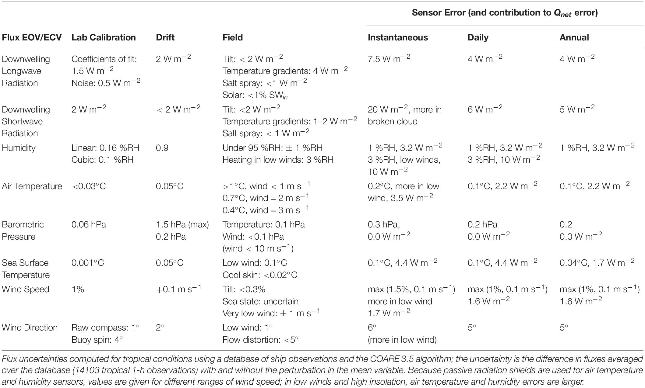
Table 1. Summary of flux EOV/ECV uncertainties based upon ASIMET sensor uncertainties stemming from laboratory calibration, sensor drift, and field impacts with estimates of total uncertainties in instantaneous, daily, and annual values (after Colbo and Weller, 2009).
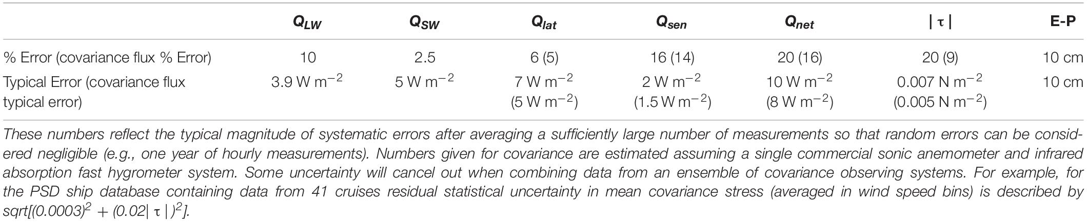
Table 2. Accuracy of long-term average of heat flux components, net heat flux, wind stress magnitude, and freshwater flux for an ASIMET system deployed in the subtropics, after Colbo and Weller (2009).
Researchers have recently begun collecting year-long time series of direct covariance flux measurements of momentum, heat and mass fluxes from surface moorings (Weller et al., 2012; Bigorre et al., 2013; Farrar et al., 2015; Ogle et al., 2018). The instrumentation on these moorings experiences less flow distortion than ships and measures a wider variety of conditions given their longer deployments. For example, fluxes were measured on a 3-m discus buoy for 15 months during the NSF CLIMODE field program. The buoy experienced wind conditions spanning 0–23 m s–1 over a wide range of stability and surface wave conditions. The fluxes measured under these conditions were used to develop the COARE 3.5 algorithm (Edson et al., 2013).
Similar flux packages have been deployed as part of NSF’s Ocean Observatories Initiative (OOI), which have been measuring motion-corrected winds for over 5 years, which will enable direct stress and buoyancy flux measurements. Recently, fast response hygrometers were used in the NASA SPURS programs (Farrar et al., 2015) to directly measure the latent heat flux. Similar work is underway to develop buoy CO2 flux systems by drying the sample. Flux systems now exist that can compute and telemeter fluxes in near real-time to shore. In general, deployment duration on buoys is limited by battery power, although some sensors are subject to biofouling and other issues that affect the calibrations. Surface buoys are also exposed to weather, vandalism, waves, and sea birds. Redundant installation of meteorological sensors is often necessary to avoid data gaps due to sensor failures. This is particularly important for flux calculations since failure of any one of the primary state variables will result in a data gap in the air-sea flux. Even with these precautions, however, surface moorings must be refreshed at 12–18 month intervals, requiring a ship to transit to these distant locations and adding to their expense. On the other hand, these mooring cruises provide an opportunity to do repeat sections to key locations in the global climate system.
Computational fluid dynamic flow studies of the buoy tower and sensors are recommended to identify errors due to flow distortion and guide improved sensor placement and tower design. Protection from marine birds is recommended. In freezing conditions, heated sensors are required to prevent ice buildup; and heating of the buoy tower maybe required to prevent ice buildup leading to tipping or inversion of the surface buoy. Of course, adding heating and ventilation as well as additional sensors to measure the fluxes directly requires increased battery payloads. This has been done successfully using isolated battery packs to deliver power on a duty cycle. The buoys of the OOI provide continuous power using additional sources that include solar panels and wind generators with rechargeable storage batteries.
The success of buoy-based systems has led to the development and use of a wide variety of platforms for observing air-sea interactions, including Autonomous Surface Vehicles (ASVs), surface drifters and spar buoys (Figure 3). ASVs generally have propulsion powered by either waves (e.g., Wave Glider) or wind (e.g., Saildrone, Sailbuoy), and have electronics powered by solar energy and/or batteries. ASVs navigation can be controlled by setting corridor width and waypoints via satellite communication system (e.g., Iridium). With speeds of up to 2.5 knots for wave-propulsion ASV and 7 knots for wind-propulsion ASV (depending upon wind and ocean conditions), and endurances of 6 months to a year, ASVs can cover thousands of nautical miles. This gives ASVs the capability to either sample in a station-keeping mode, like moored buoys, to create a fixed time series, or in repeat section-mode, or adaptive sampling mode, to do surveys like a research vessel (RV). Recent examples include sampling through hurricanes/typhoons (Lenain and Melville, 2014; Mitarai and McWilliams, 2016) and in the harsh Southern Ocean (Monteiro et al., 2015; Schmidt et al., 2017; Thomson and Girton, 2017).
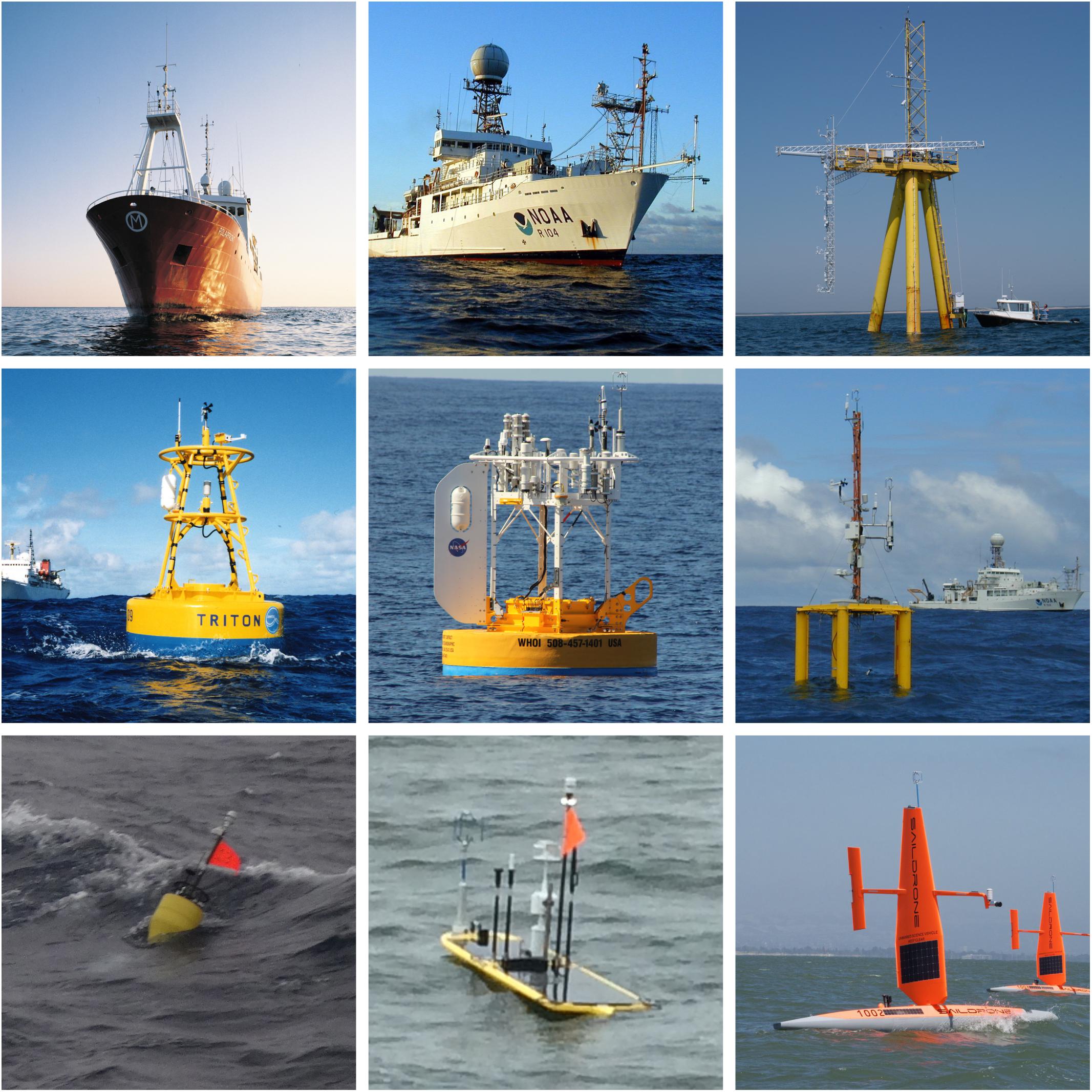
Figure 3. Examples of different types of air-sea flux in situ platforms. Clockwise from upper left: Norwegian weathership Polarfront (image courtesy of Norwegian Meteorological Institute) (Yelland et al., 2009); NOAA ship Ron Brown (from www.noaa.gov); WHOI Air-Sea Interaction Tower (image courtesy Jayne Doucette Woods Hole Oceanographic Institution); RSMAS “ASIS” spar buoy (Graber et al., 2000); Saildrone, Inc., “Saildrone” ASV (image courtesy of Saildrone, Inc.; www.saildrone.com), Liquid Robotics “Wave Glider” ASV (from www.liquid-robotics.com with modifications by UW/APL), UW/APL “SWIFT” drifter (Thomson, 2012); JAMSTEC TRITON buoy (from JAMSTEC, www.jamstec.go.jp); and, in the center, the WHOI SPURS buoy (Farrar et al., 2015).
Nearly all components for calculating bulk EOV/ECV fluxes have been measured from ASVs, including wind speed and direction, air-temperature, humidity, solar and longwave radiation, bulk temperature, skin SST, and surface currents, although some of these measurements are less mature than others. While ASVs tend to have minimal flow distortion, their platform motion (pitch, roll, heading) must be removed when transforming their measurements into Earth coordinates. Improved Global Positioning Systems (GPS) enable corrections for platform motions at better than 10 Hz. With sonic wind sensors measuring 3-dimension winds at 10 Hz or faster (particularly at high winds near the surface), field tests are underway to determine whether these platforms can be used to measure covariance flux wind stress directly in addition to the mean wind. The low height of sensors making atmospheric measurements on some of the ASVs remains a technical issue. The community also does not have a good handle on the effects of wave shadowing or distortion on the atmospheric boundary layer and its impact for example on the measured wind field (Schmidt et al., 2017) and further efforts are required to assess and address this. Quantification of the accuracy for measurements associated with air-sea heat and momentum fluxes are continuing.
ASV technology is new and currently at a pilot Technical Readiness Level (TRL) of 4 (“Trial”) – 5 (“Verification”) (Lindstrom et al., 2012). Before it can be expanded to a global array, the TRL needs to be increased to a mature TRL of 9 (“Sustained”). For this, all sensors and systems need to be validated against known standards under a wide range of field conditions on a routine basis. The platforms themselves must be understood with respect to flow distortion, height of the various instruments, and other complicating factors. Navigation needs to be automated in ways that maintain safety at sea, and enables coordinated work with other observational platforms, such as moorings, ships, and gliders (see Swart et al., 2019). Adaptive sampling of atmospheric (e.g., storms/hurricanes) or ocean (e.g., fronts and eddies) features require automatic identification and tracking by ASV. Such capability would enable optimal exploration of complex atmosphere-oceanic environments. Likewise, onboard data processing needs to be developed and tested, and sensor system, data, and metadata must be standardized. Finally, the ASV community must agree to common data delivery, archiving and best practice. An ASV governing body could help develop these standards and create an ASV network.
Drifting or Lagrangian platforms such as the ASIS (Graber et al., 2000) have been used to successfully measure the surface fluxes in field campaigns for decades. Drifting spar buoys generally require less motion correction, experience less flow-distortion and place sensors above the difficult-to-resolve processes within the wave-boundary layer (Hara and Sullivan, 2015); all of which results in accurate direct flux estimates (Edson et al., 2013; Drennan et al., 2014). Another advantage of a Lagrangian measurement of the air-sea fluxes in combination with oceanic temperature and salinity is that, to the extent the drifter follows the mean mixed layer currents, an ocean heat budget assessment can be simplified by reducing the advective flux divergence contribution to the budget (e.g., Silverthorne and Toole, 2013). Thus the surface fluxes measured by a drifter can be more directly constrained by changes in the upper ocean heat or salt content, and more directly compared to one-dimensional ocean models to evaluate the effects of surface forcing on the upper ocean (e.g., du Penhoat et al., 2002). Low-profile Lagrangian surface drifters provide reliable measurements of surface currents and waves over a wide range of conditions (e.g., Herbers et al., 2012). Recent advances in these platforms have included the ability to measure EOVs and subsurface turbulence with, e.g., SWIFT drifters (Thomson, 2012). Drifting versions of the traditional surface mooring are being developed at several institutions. These “minibuoys” provide flux measurements at significantly lower cost for field programs and could also be used to significantly augment conventional operational networks such as NDBC and TAO. The community should be encouraged to continue its efforts to design innovative platforms and flux systems while observing and developing best practices that include assessment against accepted standards.
OceanSITES Reference Time Series
The accuracy of fluxes from moorings approaches and in some casesexceeds that required for monitoring many of the ocean air-sea interaction phenomena (Figure 2). Moorings thus can provide “reference time series” for tuning satellite measurements and assessing uncertainties in satellite and NWP fields. The purpose of the OceanSITES network1 is to collect, deliver and promote the use of high-quality multi-disciplinary data from long-term, high-frequency observations at fixed locations in the open ocean. These long time-series help to distinguish variations in EOVS due to temporal variability from that due to spatial variability. The large set of co-located EOVs at these sites (e.g., surface heat fluxes, ocean wind stress, subsurface temperature, salinity, velocity, surface mixed layer depth), allow many terms in the heat, momentum and salt equations to be evaluated and thus processes responsible for variability to be identified. Such analyses are critical for identifying causes of biases in NWP reanalyses and ultimately improving the model physics.
The OceanSITES network comprises moorings funded by individual principal investigators from oceanographic agencies in many different nations. Most sites were initiated through research process studies. For example, the Stratus mooring at 20°S 85°W, was initiated during a cloud feedbacks study (Mechoso et al., 2014; Weller, 2015), while the Kuroshio Extension Observatory (KEO) was initiated during a field study of western boundary current physics (Cronin et al., 2013). Station Papa, a site of an ocean weather ship from 1940 to 1981 in the NE Pacific subpolar gyre, has been at the center of many oceanographic process studies (Freeland, 2007; Cronin et al., 2015). The NOAA surface mooring there was initiated during a process study of the carbon cycle. The WHOI Hawaii Ocean Timeseries (WHOT) mooring was initiated as an oceanic sentinel sister site to the Moana Loa “Keeling Curve.” Monterey Bay Aquarium Research Institute (MBARI) maintains a station in the California Current system. Its primary purpose is for monitoring and understanding the ecosystem productivity and biogeochemical cycling in this upwelling zone. The OOI Irminger Sea station is part of the Overturning in the Subpolar North Atlantic Program (OSNAP). The Southern Ocean Flux Station (SOFS) south of Tasmania monitors the ventilation and mode water formation in the Subantarctic Zone (Schulz et al., 2012). SOFS and the OOI Southern Ocean (50°S, 90°W) site west of Patagonia are the only two stations in the Southern Ocean. Both are subject to storms, waves, and strong currents. The Tropical Atmosphere and Ocean (TAO) mooring array in the Pacific was initiated to better understand, monitor and predict ENSO (McPhaden et al., 1998; Cronin et al., 2006), while the tropical array in the Atlantic was designed to monitor and predict both ENSO-like and meridional modes and the Indian Ocean tropical array was designed to also monitor monsoon variability (McPhaden et al., 2009). The commonality of these long time series sites is that they all are publicly available through the OceanSITES global data assembly center, in a common data format. Figure 4 shows a comparison of a satellite-based latent and sensible heat fluxes and OceanSITES moorings. Not all these moorings carry radiation sensors and therefore only a subset of these OceanSITES moorings monitor net surface heat flux.
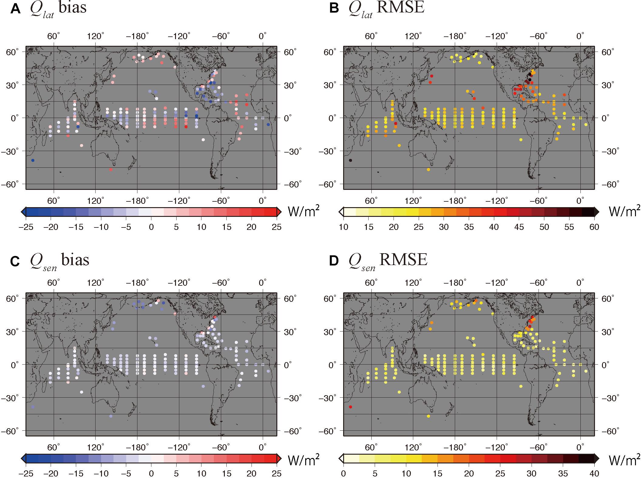
Figure 4. Comparison of J-OFURO3 air-sea heat fluxes with daily-averaged buoys for the period 2002–2013, in units W m−2. (A) Latent heat flux (Qlat) bias (satellite minus buoy); (B) Qlat root-mean-square errors (RMSE); (C) Sensible heat flux (Qsen) bias; and (D) Qsen RMSE. From Figure 5 of Tomita et al. (2019).
The long time series provided by the sustained surface moorings of OceanSITES have proven to be of high value, and continuation of the sustained observing sites is recommended. Merged, quality-controlled time series are produced at a number of such sites and have been sought after by the modeling community, by the remote sensing community (Pinker et al., 2018), and by those evaluating new hybrid flux products (Valdivieso et al., 2017). Some of the time series are just now entering a third decade of observing, and these time series are capturing accurate records of decadal variability as well as of trends. Testing whether or not models and flux products replicate the broad range of time scales in the fluxes, out to decadal and beyond, is critical and requires sustained surface flux time series of high quality. Further, detection of long-term trends and separation of trends from decadal and multidecadal variability also requires ongoing long time series. These sustained time series sites also become foci for process studies that will improve understanding of air-sea interaction and fluxes and support further improvement of models.
Within the global ocean observing system, data from OceanSITES reference stations moorings are particularly important for validating gridded products of fluxes as they provide long records of high-quality flux EOV and ECV at high temporal resolution, co-located with other EOVs and ancillary ocean variables such as the surface ocean mixed layer. In this way, the sources of the biases can sometimes be determined, leading to improvements. The suite of sensors from OceanSITES flux moorings should include not only all flux EOV/ECV, but also, if possible, direct covariance flux estimates as well, although this may require technological development for the platforms. Likewise, sea state EOVs are being tested as flux EOVs and therefore should be included if possible. In addition, it is strongly encouraged to obtain additional environmental parameters which could help represent atmospheric and oceanic conditions that may affect the air-sea exchanges and their impacts. For example, Global Navigation Satellite System (GNSS) receiver, could provide precipitable water vapor, which has been shown to improve weather forecasts (Li et al., 2015).
Current EOV/ECV observations all suffer from different drawbacks. Comparison of point measurements from in situ instruments to satellite measurements, which inherently represent an average over some spatial footprint that is typically kilometers or more in extent, is made difficult by the differences in spatial and temporal sampling. These differences, caused by spatial variability on scales smaller than the satellite footprint, can be compensated somewhat by temporal averaging of the in situ data to effectively attenuate the small-scale variability (e.g., May and Bourassa, 2011; Lin et al., 2015), but the difference in time-space averaging in different observational approaches remains a fundamental difficulty. The in situ moored buoy data is accurate and has high temporal resolution, often for a long record, but these point measurements tend to be too sparsely distributed for mapping spatial patterns and understanding teleconnections. The moored buoys tend to be located along coastlines where they are easier to maintain, and in the three main tropical arrays. Furthermore, while the surface moorings that contribute to OceanSITES and coastal arrays and to research endeavors provide many flux EOV and ECV, few measure all. In particular, only a small subset of these moorings measure solar radiation and not all of these sites measure downward longwave radiation. Likewise, surface current observations are available at only a small subset of surface mooring sites. There are also large gaps in the center of ocean basins and at high latitudes, especially in the Southern Hemisphere (see Swart et al., 2019). There are currently only 22 operating sites in this global network that measure net surface heat flux, with only 7 of those being in the Southern Hemisphere. This drastically undersamples important ocean-atmospheric regimes that are known areas of high error for flux analyses. These long, high-quality time series are critical data for satellite algorithm developers, for model testing and development, and for analyzing critical processes in the climate system. These large gaps in coverage reduce the efficacy of the observation for the research and weather applications discussed in section “Introduction.”
Current Capabilities for Remotely Sensed Flux EOV/ECV Measurements
The current capabilities for remotely sensed flux EOV/ECV are summarized in Table 3 and Figure 5. In particular, typical uncertainty estimates for the highest resolution swath products as well as high resolution gridded products. These uncertainty estimates are presented along with their contribution to uncertainty in the net surface heat flux, estimated by linearizing Eq. 1.1 with respect to the EOV/ECV following Cronin et al. (2014). It should be noted that these uncertainties are based upon comparisons to buoys, which are primarily located in the tropics. Table 3 also describes the typical spatial and temporal resolution, and where technology developments are necessary. Figure 5 shows the status of the constellation for each EOV/ECV over the next decade, and actions needed for improvement. The status of each system is described briefly here.
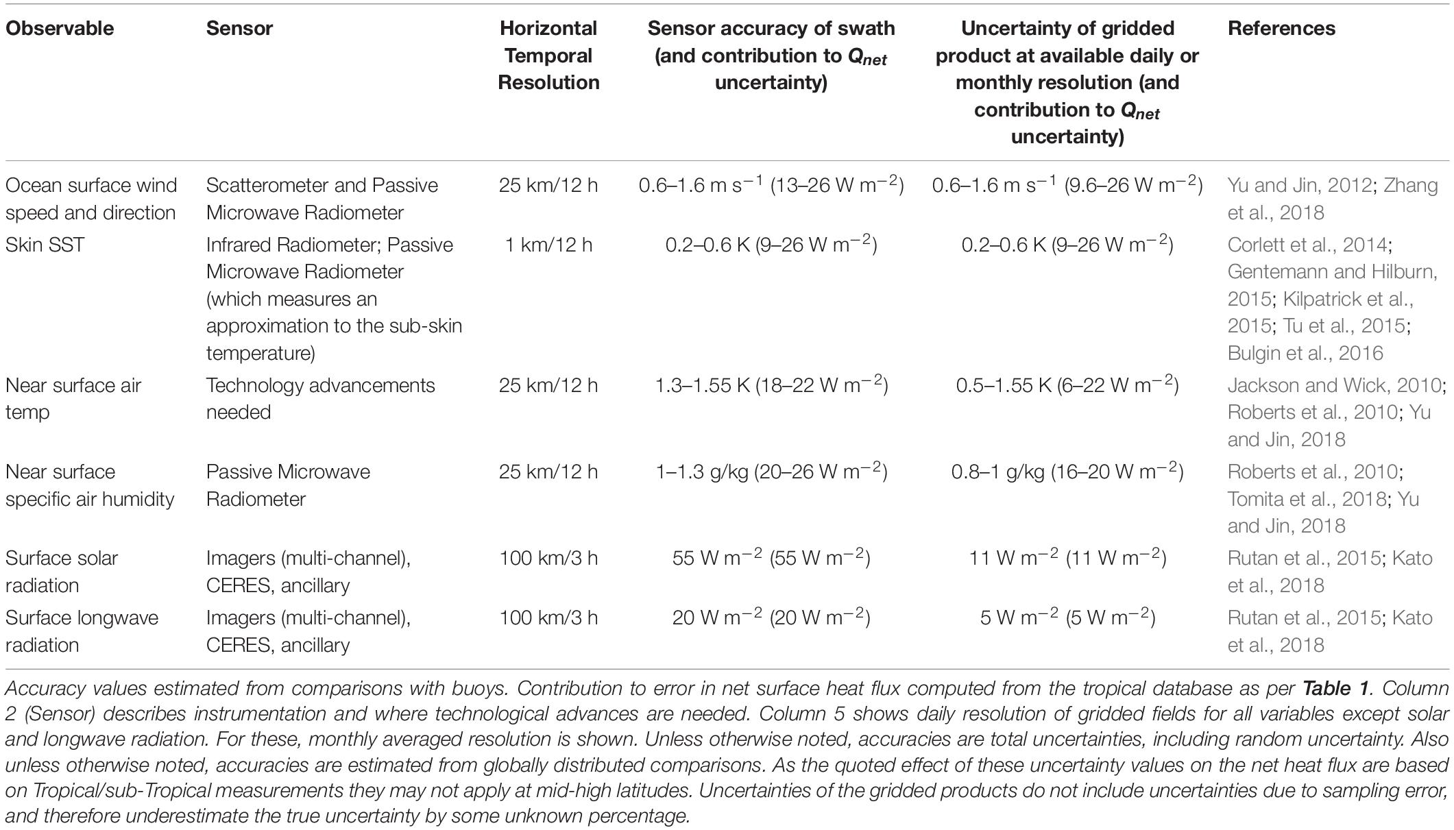
Table 3. Current capability in remotely sensed flux EOVs and corresponding error in net surface heat flux and wind stress.
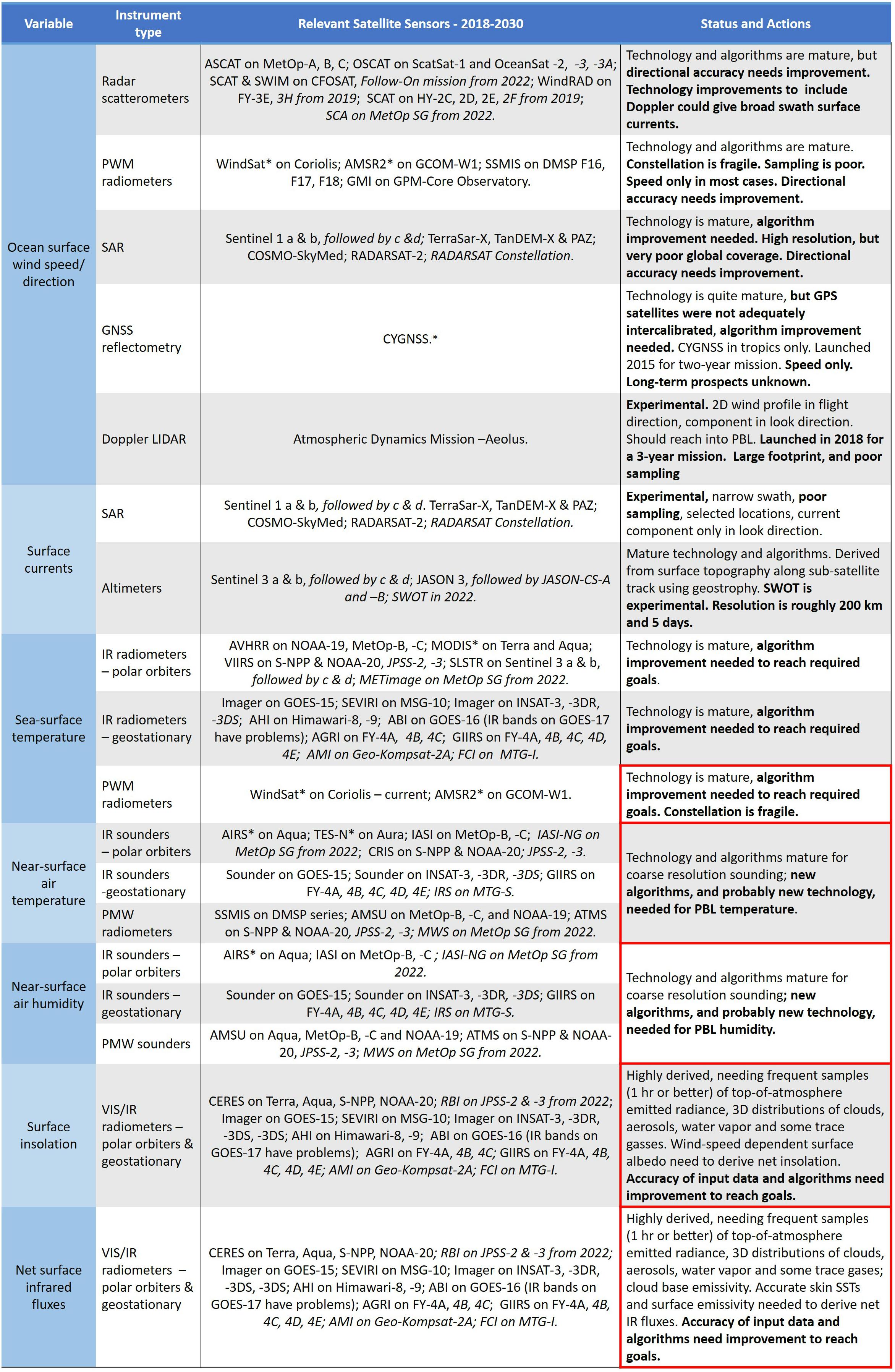
Figure 5. Satellite sensors that are producing data that can be used in deriving estimates of ocean surface fluxes. Normal text indicates current satellites and sensors, with * indicating those that are beyond their planned lifetime. Italic font shows missions that are expected to be launched in the next decade. Bold text shows areas needing attention in coming decade; red borders highlight where significant action and progress are needed. Not all derived variables from all sensors will reach the accuracies given in Table 3.
The ocean surface roughness measured by satellite sensors is normally transformed into an ocean wind speed at 10 m height using algorithms developed through comparisons with ocean buoys and NWP products (Meissner and Wentz, 2012; Shibata, 2012; Meissner et al., 2014; Hirahara et al., 2015). In reality, the ocean surface roughness is related to the air-sea velocity difference, which is actually the variable of most interest for flux calculations. The measurement of ocean surface roughness from scatterometers (e.g., ASCAT, QuikSCAT, RapidSCAT) and passive microwave (MW) radiometers (e.g., SSMI, SSMI/S, WindSAT, AMSR-E, AMSR2) is already at a spatial resolution and accuracy sufficient for most global flux estimates. At NDBC, TAO, and PIRATA buoys, monthly mean satellite wind speeds are found to have average biases of 0.3 m s–1 and RMS of 0.73 and 0.81 m s–1 (QuikSCAT and SSMI, respectively) (Wallcraft et al., 2009). RMS is a bit larger for the daily mean wind speed; RMS of 1.25 m s–1 at TAO buoy is reported (Hirahara et al., 2015). It is even larger in the Kuroshio Extension region; RMS is 1.6 m s–1 at KEO buoy for AMSR2 (Tomita et al., 2015).
The recent generation of satellite SST sensors (e.g., VIIRS, AATSR and its successor, SLSTR) are close to meeting the global uncertainty of 0.3 K for surface skin temperature measurements, but the uncertainty has regional non-random characteristics that may not always meet the uncertainty requirements (Petrenko et al., 2014). There have been efforts to generate a stable SST record (e.g., ESA Climate Change Initiative for SST, NOAA Pathfinder AVHRR, MODIS – VIIRS). In regions with persistent, seasonal cloud cover, observations are simply not possible from IR instruments, which hinders the accuracy of daily and monthly SST analyses (Liu and Minnett, 2016). Other sources of error, such as water vapor and atmospheric aerosols have regional and temporal characteristics that will impact the uncertainty (Luo et al., 2019). Passive microwave SSTs approximate to the sub-skin value, but with simultaneous observation of wind speeds, and further research into transformation of these observations into a skin value, they can provide essential observations in regions where the IR observations are simply not available due to cloud cover (see section “Systematic Uncertainties Near Fronts and Regions of Persistent Clouds”). Donlon et al. (2002) found the skin to subskin difference asymptotes to a value of –0.14 K for wind speeds above approximately 6 m s–1. Since subsurface temperature measurements from buoys are widely used in IR atmospheric correction algorithm development and validation, an offset of –0.17K is used as an estimate of the global thermal skin effect, so the subsurface temperatures approximate to a skin SST (Kilpatrick et al., 2015).
Near-surface air temperature is an exceptionally difficult observation from satellite measurements, as existing instrumentation cannot adequately resolve the planetary boundary layer, which has thicknesses varying from ∼500 m to 3 km over the ocean (von Engeln and Teixeira, 2013). This observable is currently estimated using atmospheric sounders and hyperspectral sensors, both of which have drawbacks. The sounders have higher sensitivity to the upper, rather than lower, atmospheric temperatures and have low vertical resolution, making the measurement of near surface temperature exceptionally challenging. The hyperspectral instruments such as AIRS and IASI, have high spectral resolution and offer better vertical resolution, but still suffer from the fundamental physical problem that the vertical resolution of derived profiles is limited to ∼1 km. The use of passive MW imagers to determine near-surface air temperature and humidity has been undertaken with some success, if a first-guess SST is used, with small (<0.1°C) bias and roughly 1.5°C RMS (Roberts et al., 2010; Clayson and Brown, 2016).
Near-surface air humidity is very difficult to infer accurately from satellite radiometers, for the same reasons as for near-surface air temperature. For both temperature and humidity, the weighting functions used for retrievals are dependent on the temperature and humidity profiles and, consequently, cannot be fixed for given wavelengths. Thus, there is a risk that the near-surface variables are artificially correlated with the sea-surface temperature and the state of the atmosphere, and distinguishing the true physical correlations from those that are artifacts of the measurement is difficult. In addition, the retrieval algorithms for near-surface temperature and humidity are commonly trained with in situ buoy and/or ship measurements. The relationship between satellite measurements and near-surface variables is strongly regime dependent, displaying a step-like transition (or separation) from the warm/humid regime to the cold/dry regime (Yu and Jin, 2018). The evidence suggests that the skill of the retrieval algorithm is highly dependent of the vertical distribution of water vapor. Current remote-sensing algorithms to derive near-surface humidity using a satellite MW radiometer show RMS disagreements of ∼1.0 g kg–1 with smaller positive bias in mid-latitudes (Tomita et al., 2018). A recent regime-dependent approach that treats the warm/humid and cold/dry regimes separately shows noted improvement with RMS of 0.8 g kg–1 for air specific humidity and 0.5°C for air temperature (Yu and Jin, 2018).
As discussed in section “Radiative Heat Flux EOV/ECV,” surface radiative fluxes are computed using radiative transfer models with input provided by cloud properties retrieved from satellites combined with temperature and humidity profiles. Comparisons of in situ surface observations and satellite-derived irradiances are used to estimate the uncertainty in satellite-derived irradiances; there are however, only a limited number of radiation measurements over the global ocean and most of these are in the tropics. Comparisons reported by Kato et al. (2018) show that surface monthly mean downward fluxes agree with observations to within a mean difference (RMS) of 5 (11) W m–2, respectively for shortwave, and 2 (5) W m–2 for longwave, when the differences are averaged over 46 ocean sites. Rutan et al. (2015) using CERES Edition 3 3-hourly products found an RMS of 55 and 20 W m–2 for SW↓ and LW↓, respectively. These root-mean-square differences between observed and satellite-derived 3-hourly and monthly mean irradiances are used for the uncertainty shown in Table 3. These are within the reported monthly averaged uncertainty of observed radiative fluxes at buoys of ∼5 W m–2 (Colbo and Weller, 2009). Comparison uncertainties are influenced by atmospheric, cloud and aerosol properties as well as temporal and spatial sampling issues. Ambient conditions, such as aerosol deposition, have also been shown to degrade buoy radiative flux measurements as well (Foltz et al., 2013). Although satellite derived surface radiative fluxes agree with observed radiative fluxes at buoys to within the uncertainty, most buoys are located in the tropics. To evaluate satellite derived radiative fluxes in a wide range of atmospheric conditions, observations in mid- and high-latitude regions are needed.
Systematic Uncertainties Near Fronts and Regions of Persistent Clouds
Because persistent clouds can form at fronts, IR satellite SST observations (e.g., AVHRR, MODIS, VIIRS …) can be spatially patchy due to contamination by clouds. Conversely, IR data cloud screening algorithms can also mischaracterize actual IR-observed ocean SST variability near fronts as being cloud (Kilpatrick et al., 2019). A separate issue near fronts stems from the fact that the 25–50 km spatial footprint of microwave satellite SST retrievals often exceeds the frontal scale. Furthermore, these larger footprints and antenna side-lobes can allow land contamination to impact SST front detection in coastal regions. At present, many mapping products interpolate through these patches (e.g., Reynolds et al., 2013), leading to western boundary current fronts that are too smooth and that do not capture the mesoscale variability associated with the meandering of these fronts. Because the atmospheric response depends upon the sharpness of the SST gradient (Chelton et al., 2004; Minobe et al., 2010; Parfitt et al., 2016), this bias can result in a cascade of errors. Even multi-satellite merged data are unlikely to eliminate the gaps in surface variables completely in part because of land contamination in coastal microwave-based measurements, although a proposed higher resolution sensor could mitigate this problem (e.g., Bourassa et al., 2019; Rodríguez et al., 2019).
A strategy must be developed for handling patchy data in frontal and coastal regions, using alternative data sources. While drifters, ASVs and underway ship measurements may be able to fill these gaps at times, they are likely to be too sparse both in time and space to fill all gaps. Repeat sections from these platforms, however, may provide structure functions for sharp fronts, which when combined with information about the location of the front from altimeter and tidal data, could then help fill the gaps in the patchy data with properly located sharp fronts in flux EOV and ECVs fields. Ultimately, regional atmospheric modeling, preferably with non-hydrostatic model settings and high-resolution NWP products must be used to fill in remaining patches in data with dynamically consistent fields.
Systematic Uncertainties Due to Inadequate Sampling of Diurnal Variability and Episodic Events
Satellite instruments can provide global or near-global coverage, but the spatial coverage comes at the cost of reduced temporal resolution. Many of the satellites used for estimating surface fluxes are in sun-synchronous polar orbits. Polar orbits have the virtue of providing near global coverage, and sun-synchronous orbits have significant engineering advantages, as satellite observations are made within a narrow range of local times so that solar angles and sun glint are relatively consistent at all times. For some variables, such as SST, geostationary satellites are also useful, with the advantage of providing higher temporal sampling rates that can resolve the diurnal cycle of SST. SST can vary by more than 2–4 K over the course of a day in regions of high solar insolation and low winds. Resolving only nighttime SST can lead to biases of up to 5–10 W m–2 in the long-term mean heat fluxes (Clayson and Bogdanoff, 2013).
Resolving the diurnal cycle is particularly important since the diurnal cycle in solar radiation leads to an afternoon near-surface stratification that can trap surface forcing into a thin layer. As a consequence, rain-puddles formed during the daytime are fresher than ones formed at nighttime (Cronin and McPhaden, 1999). Likewise, “diurnal jets” can form, with anomalous wind-forced surface currents that are stronger in the afternoon than at nighttime (Cronin and Kessler, 2009, their Figure 5). The afternoon near-surface stratification also traps surface heat fluxes, making them more effective at causing SST change than at nighttime when the mixed layer depth is deeper. The diurnally varying mixed layer depth, in this way, causes rectification of diurnal variability into longer timescales (Bernie et al., 2005).
Satellite and NWP/reanalyses fluxes may also be biased due to poor representation of short-term extreme flux events associated with very strong winds and strong temperature and humidity gradients near the surface. In satellite-based fluxes these biases are likely due to poor sampling while in NWP and reanalyses they also might be associated with inability of atmospheric models to adequately simulate such conditions. Bentamy et al. (2017) using probability density function approach (Gulev and Belyaev, 2012) demonstrated that extreme fluxes derived from satellite products may deviate from flux extremes estimated from buoy measurements by tens of W m–2, even if the mean flux estimates are comparable.
Except at high latitudes, a single polar orbiting satellite can provide a maximum of two measurements per day (e.g., at 10:30 am and 10:30 pm), which is inadequate for resolving atmospheric synoptic variability or for resolving the amplitude and phase of the diurnal cycle. The diurnal cycle can be resolved by either placing several satellites in different sun-synchronous orbit planes to sample several discrete local times or by a single satellite in a lower inclination orbit. In the latter case, the satellite will precess through the diurnal cycle for any location on the ground over a period of time (days to months) that is related to the orbit inclination. Placing several satellite in sun-synchronous orbits, while more costly, has the benefit of sampling the diurnal cycle daily at discrete local times and reduces the overall re-visit time for resolving rapidly evolving storms and short-lived extreme events.
Current Capabilities for Gridded Flux Products
To create the global flux products, the flux EOVs and ECVs must be observed or estimated with sufficient resolution and coverage to map their fields, or to constrain NWP model solutions and reanalyses to produce realistic flux fields. For flux products that extend back to the early-mid twentieth century, these gridded products based upon observations and NWP rely exclusively upon in situ data, primarily from underway ships. In the past decades, a satellite constellation has been building that can provide several of the gridded EOVs necessary for creating the flux products. However, because satellites are at present unable to provide some EOVs (e.g., surface air temperature and humidity) with acceptable accuracy, for some “blended” products such as the OAFlux product (Yu and Weller, 2007), air temperature and humidity are instead based on bias-adjusted NWP outputs, while other flux EOVs and ECVs are derived from satellite data. Satellite measurements appear to provide sufficient signal-to-noise ratios to produce high-quality stress estimates; however, direct in situ measurements of stress are too sparse to provide adequate calibration. The common practice is to derive winds from satellite backscatter measurements by utilizing in situ wind measurements and compute wind stress from bulk flux parameterization.
Even NWP and blended flux products, however, have large biases and uncertainties (Cronin et al., 2006; Bentamy et al., 2017; Valdivieso et al., 2017; Tomita et al., 2019; Yu, 2019). Mean fields from 12 products show standard deviations of up to 30 W m–2 for net surface heat flux and 5 × 10⁻² N m–2 for wind stress (Figures 1C,D). It should be noted though that agreement between the different products does not mean that there are no biases; it may mean that all products are biased in the same way. In this case, the standard deviation around the multiproduct mean is not an appropriate estimate of the uncertainty. Moreover, the standard deviation could be overestimated due to outlying products. Thus, independent reference data are required to determine the accuracy of these products.
For the global average, ocean heat content estimates show the net surface heat flux into the ocean to be less than 1 W m–2 (e.g., Roemmich et al., 2015); for most products, the global average of the net air-sea heat flux is up to an order of magnitude larger than this (Figure 6A and Table 4). Comparisons of the state variables against moored reference station data show that a substantial part of this mean bias is due to deficiencies in the bulk algorithm used by the NWP (Jiang et al., 2005; Zhang et al., 2016). Bias can also be associated with the radiative heat flux components (Figure 6B), highlighting the need to improve satellite radiative observations and the presence of clouds in NWP. In order to understand the regional distribution of these errors and diagnose their causes, in situ reference stations are needed (Figure 4).
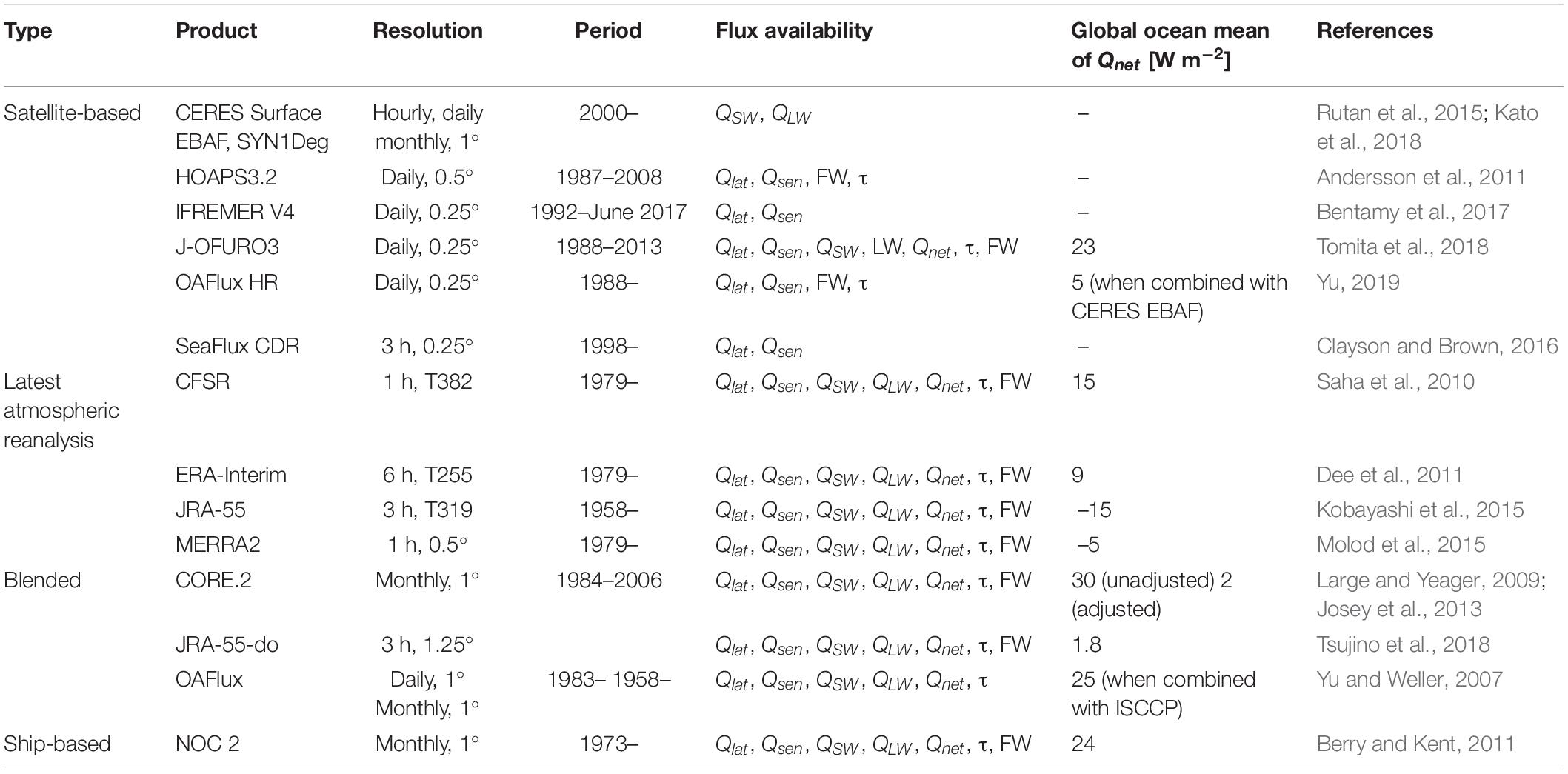
Table 4. Various flux products information (based on Bentamy et al., 2017; Valdivieso et al., 2017; Tomita et al., 2018; Yu, 2019), including temporal and horizontal (in degrees) resolution, period of availability, flux components [Shortwave (QSW), Longwave (QLW), Sensible (Qsen), Latent (Qlat), Net air-sea heat flux (Qnet), Freshwater Flux (FW), and Momentum flux (τ)], and global ocean mean value for Qnet where available.
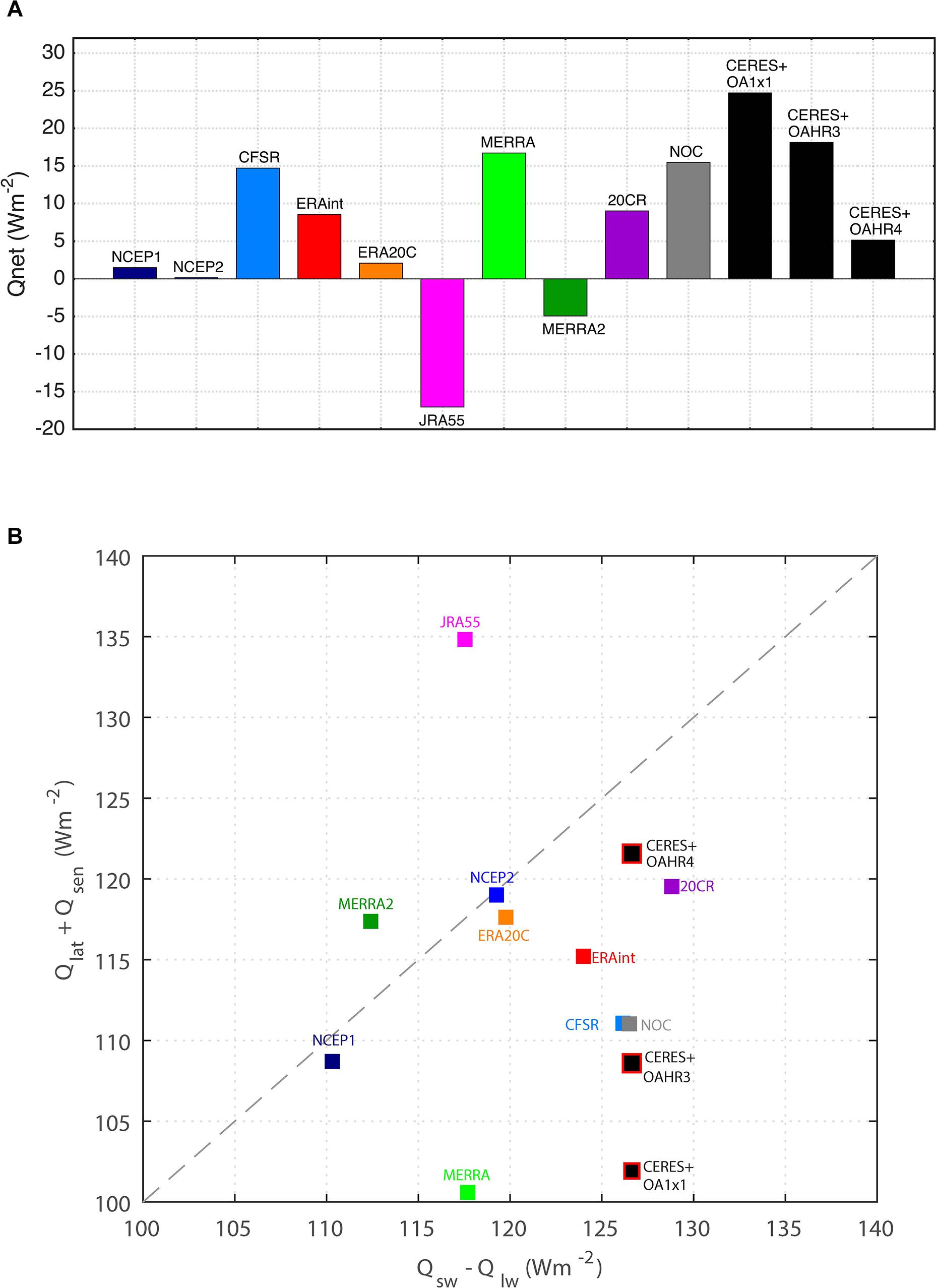
Figure 6. (A) Global-ocean mean energy (Qnet) budget. (B) The ratio of the mean averages of QSW - QLW to Qlat + Qsen; the dashed line denotes that this ratio equals 1.0. Abbreviations: 20CR, Twentieth Century Reanalysis; CERES, Clouds and the Earth’s Radiant Energy System–Energy Balanced and Filled; CFSR, Climate Forecast System Reanalysis; ERA-20C, European Centre for Medium-Range Weather Forecasts Twentieth Century; ERA-Interim, European Centre for Medium-Range Weather Forecasts Interim; GPCP, Global Precipitation Climatology Project; JRA-55, Japanese 55-Year Reanalysis; MERRA, Modern-Era Retrospective Analysis for Research and Applications; NCEP, National Center for Environmental Prediction; NOC, National Oceanography Centre; OAFlux-1 × 1, 1°-gridded Objectively Analyzed Air–Sea Fluxes; OAFlux-HR3 and -HR4, high-resolution (0.25°-gridded) Objectively Analyzed Air–Sea Fluxes analysis computed from Coupled Ocean–Atmosphere Response Experiment (COARE) version 3 and version 4, respectively. The 12 products used here are the same as used in Figure 1 from Yu (2019).
To improve NWP fluxes, marine boundary layer physics in NWP must be improved, including their algorithms for computing air-sea fluxes. In addition, more in situ and remotely sensed data with higher accuracy are needed to constrain the NWP. More accurate satellite-based moisture and temperature profiles and surface data would greatly improve remotely sensed estimates of surface radiation and latent and sensible heat fluxes, and if assimilated into NWP models, would likely lead to improved representation of cloud formation processes and thereby improved representation of the state variables and surface radiative and turbulent fluxes from these NWP models.
Aspirational Sampling Requirements and Target Uncertainties
Air-sea fluxes are challenging to observe because high-frequency variability and gustiness rectifies into the longer time scales. To adequately represent the annual cycle of heat fluxes, synoptic variability associated with storms must be captured. Subdiurnal resolution is required to adequately represent fluxes associated with fast-moving storms or in regions with a large diurnal cycle in SST. Fast moving atmospheric synoptic transients are associated with surface flux extremes (e.g., Tilinina et al., 2018), which can only be resolved in high resolution data. A gridded air-sea flux product that has 25 km or better spatial resolution and at least 3-hourly temporal resolution with a random uncertainty of 15 W m–2 and a bias of less than 5 W m–2 would be able to capture most of the air-sea interaction phenomena shown in Figure 2. The corresponding wind stress product should have a random uncertainty of ± 0.01 N m–2 (or a 5% noise-to-signal ratio, whichever is larger) and a bias of <0.005 N m–2. It is important though to realize that the native resolution of the source observations for this gridded product must be at least 2–4 times better – at least 10 km and hourly. While this represents an improved accuracy at this resolution for wind stress, for the heat flux product, achieving this accuracy would represent a breakthrough advancement. Table 5 summarizes the sampling requirements for each flux EOV/ECV needed to meet this aspirational target. Because SST is the primary ocean EOV that drives the air-sea flux, and can be controlled by ocean frontogenesis processes, SST must have the highest spatial resolution of all EOV/ECV. We set an aspirational target of 1 km. This aspirational target, even now, is partially met for many parts of the global ocean.
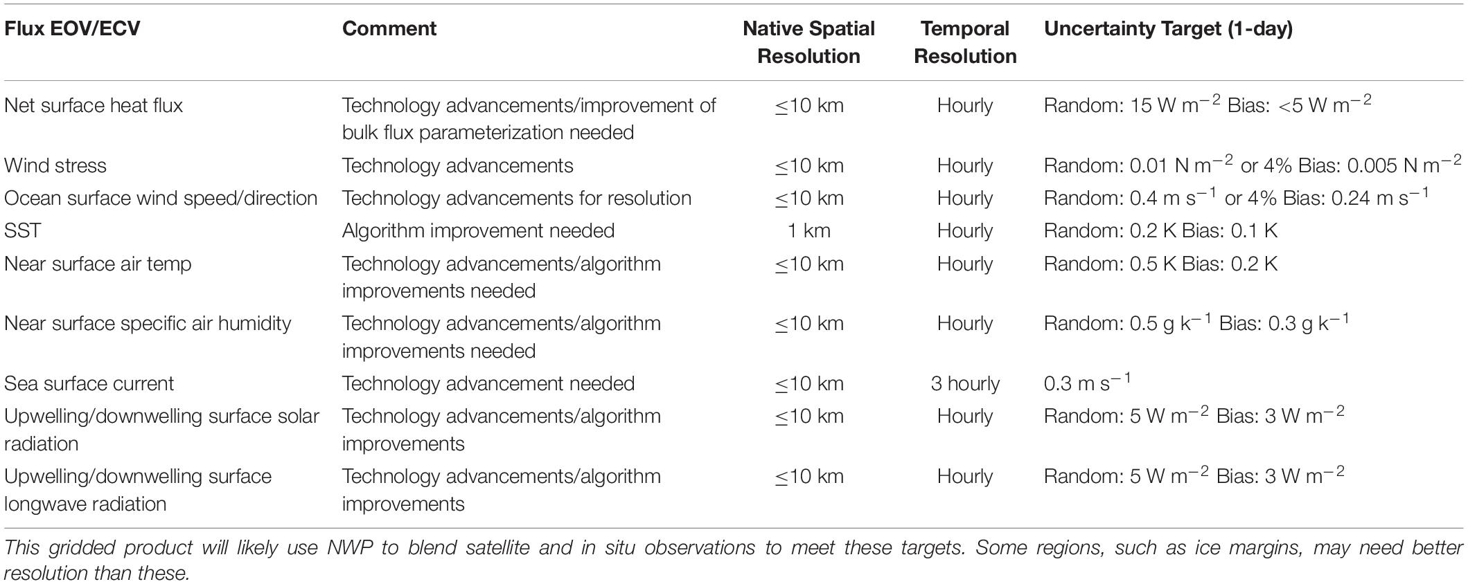
Table 5. Sampling and uncertainty targets for producing a 3-hourly 25-km (aspirational goal of hourly at 10-km) gridded product of Qnet with a 1-day random uncertainty of 15 W m–2 and a bias of less than 5 W m–2.
Opportunities for Improved Fluxes in the Global Ice-Free Ocean
For global ice-free ocean estimates of turbulent heat and momentum fluxes, it is necessary to measure the flux EOVs and ECVs with sufficient accuracy, coverage and resolution to meet the targeted uncertainty and stability. As described in section “Current Capabilities,” the primary state variables for computing turbulent air-sea fluxes of heat and momentum include near surface air temperature, ocean skin SST, near-surface humidity, and the surface wind relative to the ocean surface currents. At present, humidity and air-temperature ECVs do not meet the requirements needed for global flux estimation (Tables 3, 5 and Figure 7). Our two major recommendations, described below, and our roadmap to flux improvement described in section “Roadmap for Improving Air-Sea Fluxes,” will address these deficiencies and others, enabling adequate sampling for all primary flux EOV/ECV by 2030.
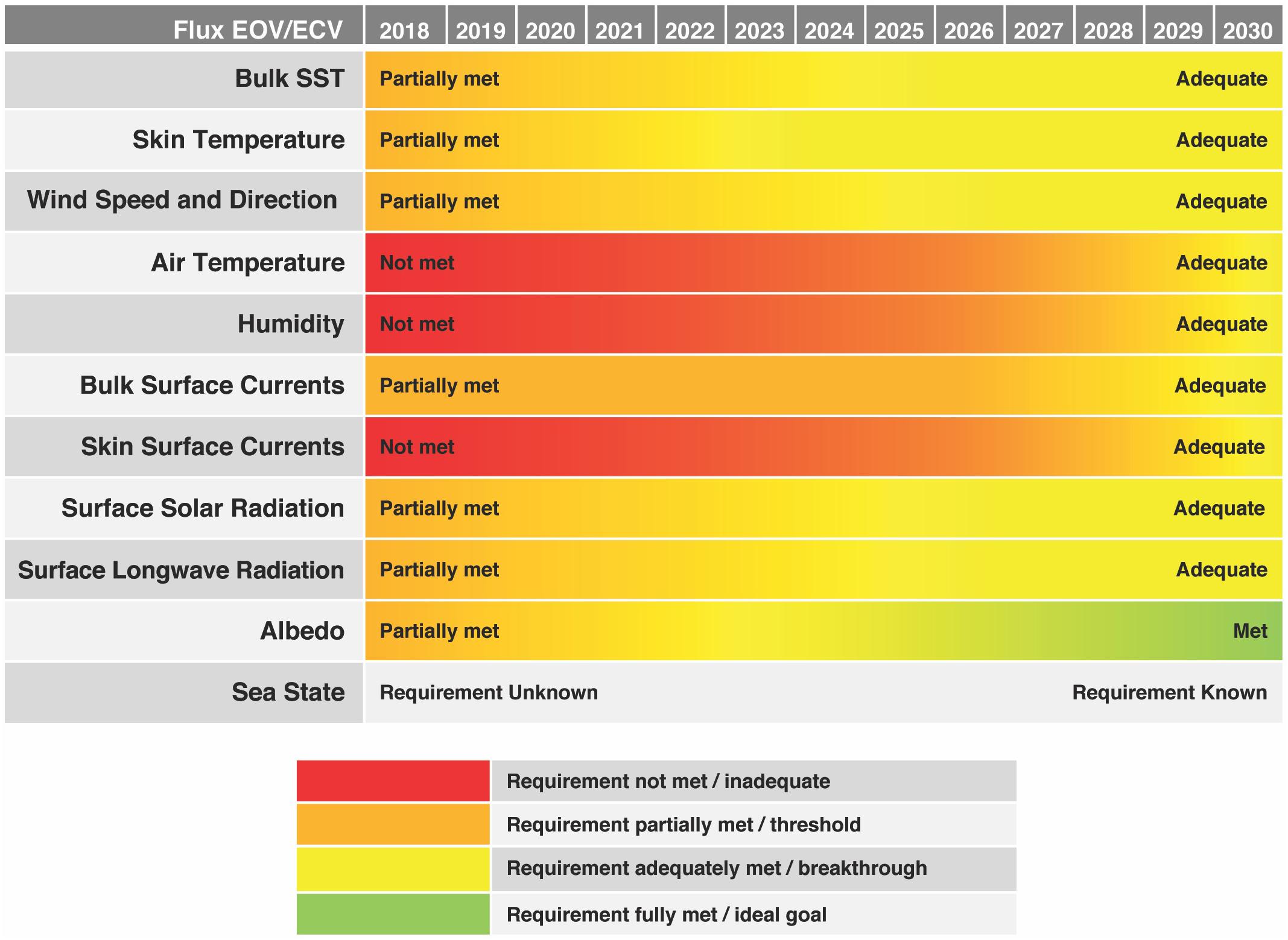
Figure 7. Overall status of flux EOV/ECV, assuming recommendations made here are followed.
Space-Based Sensor for Near Surface Moisture and Air-Temperature Retrievals
A future remote-sensing measurement system designed for the boundary layer can address many of the issues that bedevil the present system. In particular, as described in section “Current Capabilities for Remotely Sensed Flux EOV/ECV Measurements,” existing remote sensing satellites are able to measure near surface wind speed and surface skin temperature with sufficient accuracy using either microwave or IR instruments, although further algorithm development is needed since these measurements are often tuned to bulk (rather than skin) SST and wind speed (rather than wind stress). Current atmospheric sounders are able to measure vertical profiles of temperature and water vapor, and these observations are the basis for deriving satellite-based near-surface air temperature and humidity.
Three major challenges need to be addressed to improve remotely sensed estimates of heat fluxes: improvements to retrievals, improvements to time coincidence of EOVs/ECVs, and improvements to algorithms. The first challenge is to improve the sensitivity and vertical resolution of microwave sounders in the boundary layer. Existing microwave sounders typically only have a few channels giving sensitivity at less than 10 evenly spaced levels from the surface to 20 km for temperature and to 10 km for water vapor. These channels are also fixed in frequency and often introduce biases due to the shift of the weighting functions (see section “Current Capabilities for Remotely Sensed Flux EOV/ECV Measurements”). This may be overcome by adding additional channels, such as hyperspectral microwave sounding spectrometers at 50 and 183 GHz. Simulations of a notional hyperspectral sensor with a neural network retrieval algorithm predict uncertainties of 0.6°C for near-surface air temperature and 7% error for near-surface specific humidity, effectively doubling the accuracy of existing retrievals, for 1 km layers from the surface to 10–20 km altitude (Blackwell, 2005; Blackwell et al., 2011; Boukabara and Garrett, 2011). Assimilation of these better-resolved profiles into NWP should lead to additional improvements to the representation of near-surface conditions and thus air-sea fluxes.
The second challenge is to improve the time coincidence of the remotely sensed flux EOV/ECV measurements, which are typically made by independent systems and therefore usually not coincident in time, introducing de-correlation errors when computing fluxes from merged data. Time coincidence could be achieved by combining instruments on the same platform, or by using instruments on separate platforms flying in formation, which would most likely require a set of small satellite sensors to be cost effective. Alternatively, a passive microwave radiometer that combined low-frequency window channels used to measure SST and wind speed with atmospheric temperature and water vapor sounding channels would address the co-incidence issue with a single instrument. Radiometer instrument technology has made rapid strides in the past several years to miniaturize and lower the cost of the sensors envisioned for this constellation, coupled with equal advancements in low-cost CubeSat and small satellites. The US Air Force plans to demonstrate a low-cost conical microwave imager (Brown et al., 2017) and NASA has two missions to demonstrate CubeSat microwave imager/sounders (Reising et al., 2016; Blackwell et al., 2018). In addition, launch costs have decreased through rideshare opportunities.
The third challenge is to improve the retrieval algorithms for near-surface air temperature and humidity. While SST and wind speed accuracies are typically better than 0.3–0.5°C (Gentemann, 2014; Kilpatrick et al., 2015) and 0.5–1.4 ms–1 (Zhang et al., 2018), direct retrievals of near-surface air temperature and humidity a few meters above the sea surface remains challenging. Remote sensing retrievals provide average values for the lower 1 km. The relationship between this average and the air temperature and specific humidity at the sea surface requires an understanding of the vertical distribution of moisture within the atmospheric boundary layer and how this varies regionally and temporally. The suggested roadmap therefore includes a holistic program to improve and tune the retrieval algorithms and our understanding of their uncertainties, which will require improved remote sensing observations and a global array of in situ observation.
Globally Distributed in situ Network of Flux EOV and ECV
As discussed in section “Current Capabilities for Remotely Sensed Flux EOV/ECV Measurements,” the sparsity of the in situ network of flux EOV/ECV observations, particularly in large regions of the Southern Hemisphere, stands as a major obstacle to progress. Lack of in situ data in these regions and other regimes lead to large uncertainties in satellite air humidity and temperature retrievals because retrieval algorithms are not sufficiently trained to represent various near-surface boundary conditions (Yu, 2019). In regions of low winds, where SST can have a large diurnal cycle and wind gustiness contributes significantly to the wind variance, in situ surface observations may capture the temporal variability of air-sea fluxes better than polar-orbiting satellite. Likewise, in situ observations may be better at capturing temporal variability of fast moving storms in the northern and southern hemisphere storm tracks. These tend to be regions with convective rainfall, which also can contaminate satellite IR scatterometer measurements. Finally, while satellite observations have a spatial resolution that a global in situ array could never meet, as discussed in section “Systematic Uncertainties Near Fronts and Regions of Persistent Clouds,” satellite can have data gaps due to persistent clouds in frontal regions precisely where air-sea fluxes are expected to be large. Together, these strengths and weaknesses of remotely sensed vs. in situ observations argue for developing a global in situ flux-observing array to complement the global remote-sensing constellation.
Mazloff et al. (2018, their Table 1) provide estimates for heat and carbon flux decorrelation scales in the Southern Ocean, sorted into low-pass and high-pass scales. The low-pass requirements need very sparse sampling (90° by 10°; 11 measurements), but high-pass sampling is more substantial: 156 measurements in the 70° to 35° latitude range, or roughly one measurement per 4° by 4° box. Further work will need to be done to determine the optimal design of this regionally distributed plan. But at its center might be pairs or clusters of flux platforms within a regular grid (e.g., 10° by 10°) box. For reference, nodes of a 10° grid are shown in Figure 8, with 368 nodes in the global ocean. We envision a global network of flux observing platforms made up of ASVs, drifting and moored buoys, and R/Vs, with the exact choice of platform dependent upon conditions and scientific needs. This large-scale network of high-resolution sampling would ideally capture frontal structures that are critical to the generation of large exchanges of heat between the ocean and atmosphere.
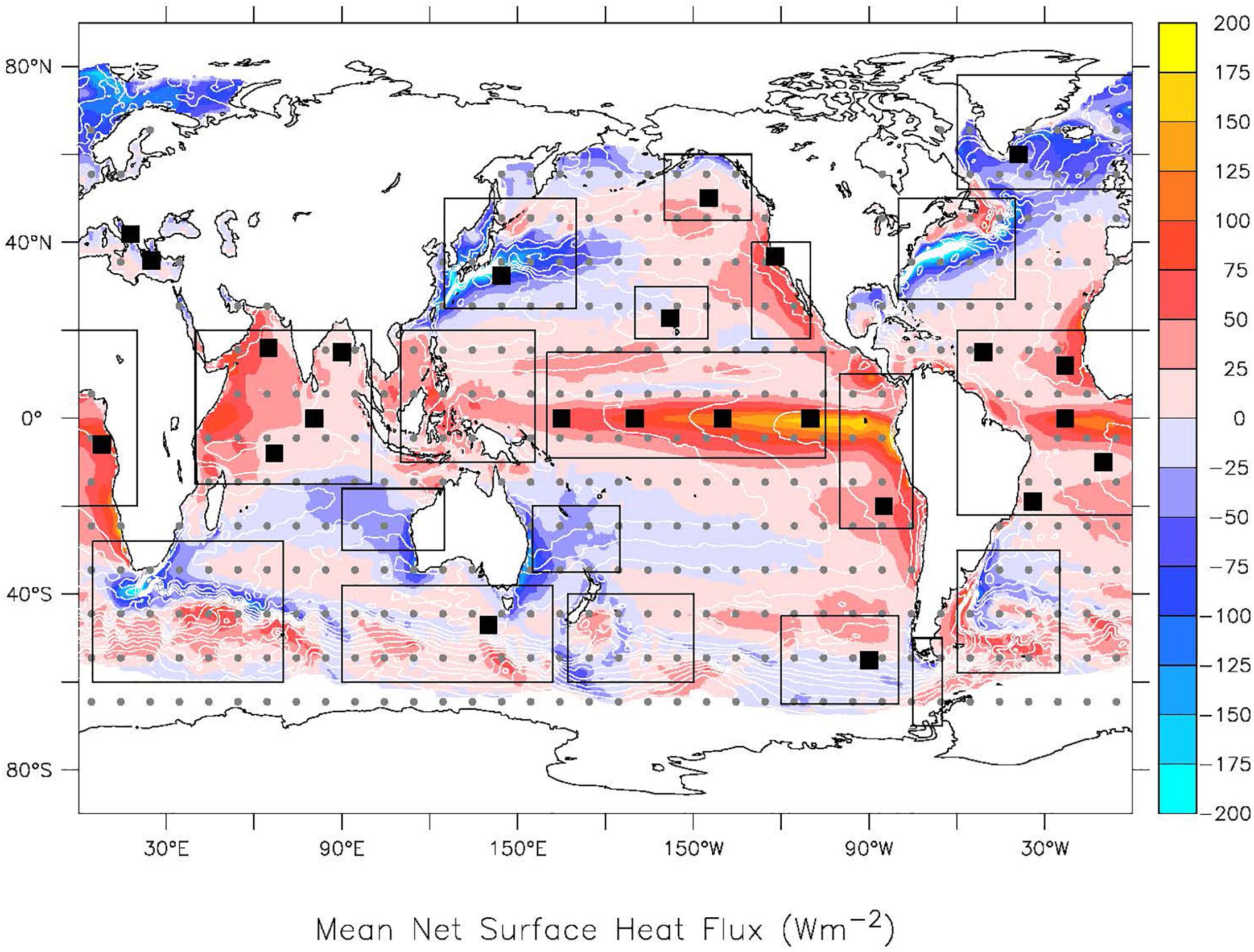
Figure 8. Existing OceanSITES network of surface heat fluxes (filled black squares) with priority regions for new OceanSITES stations indicated by black boxes. The gray dots indicate nodes of a 10° by 10° grid, with 368 grid boxes in the global oceans. The background mean net surface heat flux is constructed from OAFlux-HR (Yu, 2019) and CERES EBAF (Kato et al., 2018) for the period of 2001–2015.
These flux platforms could carry other sensor suites too, such as air-sea carbon dioxide flux packages and ocean acidification sensors. In this way, the network could be multi-functional and serve a range of communities and stakeholders beyond those described here. In the future, as true coupled data assimilation becomes standard for NWP, we would expect that this network of co-located surface ocean and atmospheric in situ observations would be particularly valuable for assimilations.
This globally distributed array should be built around an expanded OceanSITES network. At present, the OceanSITES surface flux array is too sparse, with 22 sites that measure net surface heat flux. Nineteen key regions needing OceanSITES time series stations are shown in Figure 8. These regions include eleven discussed in section “In situ Platforms for Observing Fluxes,” as well as regions in the western equatorial Pacific and western North Atlantic, and eight additional high priority regions in the Southern Hemisphere. These regions have no OceanSITES flux reference station. As discussed in section “In situ Platforms for Observing Fluxes,” an OceanSITES station not only monitors the air-sea fluxes, but also the local response of the ocean, atmosphere, and ecosystem to these air – sea exchanges. Tozuka et al. (2018) have shown that the contribution of surface heat fluxes to surface frontogenesis/frontolysis depends not just on the flux gradients, but also on the distribution of mixed layer depth, which controls the effective heat capacity of the upper ocean. The OceanSITES flux network provides these co-located air-sea flux, mixed layer depth observations, and other EOVs so that budget analyses can be performed to determine causes for surface variability.
In some regions, such as the tropical Pacific, the number of OceanSITES flux reference stations could be increased simply by adding a few sensors to existing OceanSITES surface moorings. In other regions, new mooring stations are needed. The Tropical Pacific Observing System (TPOS)-2020 project is working to optimize flux measurements in the tropical Pacific, including the eastern and western boundary regions (Smith et al., 2019). Likewise, the Southern Ocean Flux working group is in the process of developing a deployment strategy to optimize the positioning of a sparse internationally supported array of flux moorings (Swart et al., 2019). Regional groups, like these, have the scientific expertise and local knowledge that are critical for making these long-term stations successful. Nevertheless, the following list of new sites are considered to be a high priority as they are all in regions that do not at present have any flux reference station:
New Flux Reference Sites for 8 Key Regions with no Flux Station at Present
(1) Tropical Western Pacific (9°N, 150°E; equatorial region west of 165°E): Typhoon corridor, monsoon, intraseasonal oscillations, and ENSO variability.
(2) Southern Ocean (order 60°S, any longitude): Ice-edge conditions. Southern Hemisphere storm track.
(3) Southern Ocean (40S°–60°S, any longitude): Southern Hemisphere storm track.
(4) Agulhas (40°S, 36°E): Intense heat loss region associated with S. Indian Ocean western boundary current (WBC), extratropical storms, interbasin eddy heat exchanges, mixed layer depth role in front gradient.
(5) Southeast Indian Ocean (25°S, 110°E): Strongest ocean evaporation region (globally) in trade wind return flow, subject to “Ningaloo” mid-latitude marine heat waves. Subtropical mode water formation site.
(6) Gulf Stream (35°N, 60°W): Intense heat loss associated with N. Atlantic WBC, eddy rich region, tropical-extratropical cyclones and interactions, cold-air outbreaks.
(7) East Australian Current (35°S, 160°E): S. Pacific WBC, Tasman Front, tropical-extratropical interactions.
(8) Brazil-Malvinas Confluence (42°S, 42°W): S. Atlantic WBC, eddy rich region, tropical-extratropical interactions.
These regions listed here are high priority because they at present have no OceanSITES flux reference station in them. Our boxed regions, however, are large, covering major quadrants of each basin. Each have multiple regimes, sometimes separated by major fronts. For many regions, such as the tropics, multiple stations are justified. Careful array design studies by regional experts is recommended.
A subset of the long-term reference stations should be enhanced for process studies and to provide high resolution turbulent flux and mean profiles that extend 20 to 100 m into the marine atmosphere. These “super sites” would provide critical observations to validate and guide model physics and bulk flux and satellite retrieval algorithm development. Such a system, with multiple levels of fast-response sensors to directly measure momentum, heat and mass exchange, could be based on fixed towers, large moored spar buoys or other floating platforms, which are being developed and used by the offshore wind industry. Remote sensing systems deployed on the platforms and from nearby moorings (e.g., Lidar buoys) could provide further characterization of the coupled boundary layer, including cloud information, boundary layer height and mixed layer depth. Other key variables to be observed at these sites could include wave information, radiative fluxes (including both upwelling and downwelling fluxes), skin SST, precipitation, high-resolution upper ocean currents, fast static pressure, and a suite of oceanic boundary measurements, among others. These supersites and their associated infrastructure would also serve as testbeds for validation of innovative platforms and systems, such as low-power sensors and remote sensing systems for deployment on buoys and mobile platforms. In addition, it is recommended that some of the ships servicing the moorings and supersites be enhanced to monitor the coupled boundary layer, and host unmanned aircraft systems for observing along-wind and cross-wind variations, obtaining data to improve albedo parameterizations, and for monitoring a wide-range of coupled boundary layer processes. The breakthroughs highlighted in Figure 7 depend not only upon improved remote sensing and expanded in situ observations, but also upon improved models, algorithms and parameterizations. This ambitious goal is predicated upon vigorous research fed by these coupled boundary layer observations described here.
Roadmap for Improving Air-Sea Fluxes
Quantifying air-sea fluxes is very challenging as multiple co-located flux EOV/ECV must be measured at high temporal and spatial resolution, with high accuracy. At present, the global ocean observing system does not meet the necessary requirements (Figure 7), mainly due to the lack of global coverage of surface humidity and air temperature. Our two major recommendations rectify this and other deficiencies:
Major Recommendation #1
Create a remote-sensing retrieval system designed for accurate boundary layer measurement of air temperature, humidity, SST, and surface stress. This would involve a holistic approach to improve resolution of satellite retrievals, time coincidence of remotely sensed surface flux EOVs/ECVs, and algorithms that relate the retrievals to near-surface conditions.
Major Recommendation #2
Create a global in situ array of flux observing platforms, built around an expanded OceanSITES network of time series reference station moorings. The global array would include ∼500–1000 platforms including ASVs, moored and drifting buoys, and RVs, with 1–3 platforms in nominal 10° by 10° boxes. The OceanSITES network of 22 flux sites must be maintained and expanded in up to 19 key regions. In addition, the in situ array should include a few super sites with enhanced observations of the coupled boundary layer.
These major recommendations depend upon a number of steps taking place, as shown in the Roadmap (Figure 9):
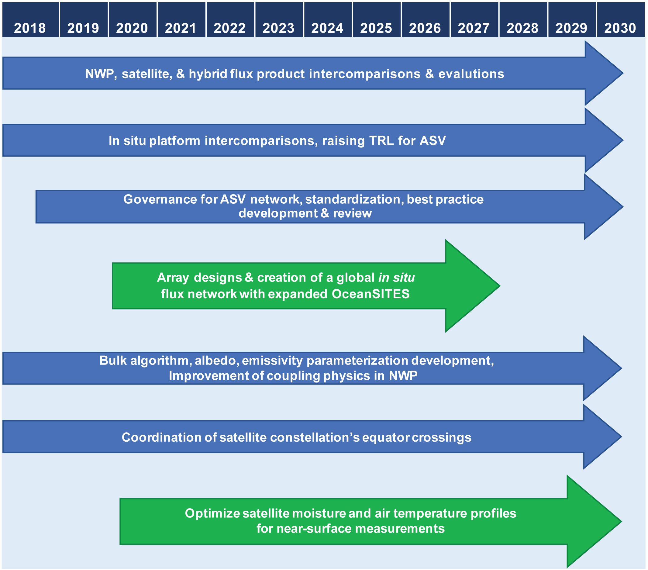
Figure 9. Roadmap chart for making improvements in air-sea fluxes over the next decade. Major recommendation activities are indicated in green. Arrows indicate that these activities are likely to be ongoing.
• The TRL for ASV and other new flux platforms must be increased before being used to form a large global network. These platforms must be continually evaluated against satellite and proven technology, including RVs, flux towers with vertical extent, and OceanSITES and OOI moorings. It is recommended that an international ASV expert group form to coordinate ASV data stream, evaluate data, and develop best practices and standardizations.
• Array designs for the in situ flux network must be studied. It is likely that a flux network would have some similarities to an Argo array in being globally distributed, but also have some distinct differences due to the importance of fronts and rapid variations in flux EOV/ECV. Likewise, in contrast to Argo, adaptive sampling capabilities of ASV could allow the globally distributed array to target certain phenomena and to sample in combination with other fixed platforms. Determining the optimal array design will require both model studies and pilot field studies.
• International coordination of data management and archival must be extended to flux-related data streams, including for all underway RV observations, ASVs, drifting and other flux platforms, and for observations transmitted in near real time in support of NWP on the Global Telecommunications System (GTS).
• With the expanded in situ array of platforms that measure all flux EOV/ECV including direct covariance flux estimates of the turbulent fluxes, the state of the art bulk aerodynamic flux algorithm can be improved, leading to reduced uncertainties. It is critical that the bulk algorithm in NWP be improved.
• Parameterizations for transforming bulk EOV/ECV into bulk algorithm state variables must be improved. These include (but are not limited to) extrapolation of bulk sea surface state variables to the air-sea interface, and parameterizations of albedo and emissivity.
• Cross-platform and cross-product intercomparisons must take place and differences must be reconciled. Sensors across all in situ platforms should have laboratory calibrations traceable to international standards, and field intercomparisons to verify consistency. Identification of field errors should lead to changes in best practices. Identification of model errors should lead to recommendations for improved physics and parameterizations.
Conclusion
In this paper, we lay out an observational strategy for producing 3-hourly at 25-km (and an aspirational goal of hourly at 10-km) gridded heat fluxes and wind stress fields over the global, ice-free ocean that have a breakthrough improvement in accuracy for heat flux and, for these scales, an improved accuracy in wind stress. The target for the net heat flux product is 1-day random uncertainty of 15 W m–2 (or 5% error for each radiative component and the sum of the turbulent heat fluxes) and a bias of less than 5 W m–2. For the wind stress product the target is 1-day random uncertainty of ± 0.01 N m–2 (or a 5% noise-to-signal ratio, whichever is higher) and a bias of 0.005 N m–2. At present the heat flux uncertainty target is met only at OceanSITES reference station moorings and RVs that follow best practices. To meet these targets in the next decade, we make two major recommendations: (1) Create a remote-sensing measurement system designed for accurate boundary layer measurements of air temperature, humidity, SST, and surface stress; and (2) Create a complementary global in situ array of flux observing platforms, built around an expanded OceanSITES network of time series reference station moorings. The global array would include ∼500–1000 platforms including ASV, moored and drifting buoys, and RVs, with 1–3 platforms in nominal 10° by 10° boxes. The OceanSITES network of 22 flux sites must be maintained and expanded in up to 19 key regions. The in situ flux array would provide globally distributed measurements and metrics for satellite algorithm development and product validation. In addition, in situ flux EOV and ECV observations that also include direct covariance flux observations could be used to improve “bulk aerodynamic algorithm” for computation of air-sea exchange of heat and momentum. With improved coupling of the ocean and atmosphere in NWP, and constrained by the improved moisture and air temperature profiles, these NWP are expected to have improved representation of cloud formation processes and radiative properties. Together, these will lead to a more accurate satellite-based (and blended) flux product. This better quantification of the ocean’s influence on the atmosphere will lead to improved long-term weather forecasts, seasonal-interannual-decadal climate predictions, and regional climate projections.
Author Contributions
MFC, CLG, JE, and IU were first authors for abstracts that were merged into the present version. MFC wrote the first draft of the manuscript. CLG, JE, SB, IU, EK, RAW, SAJ, RTP, SK, CWF, HT, PJM, JTF, SS contributed to text sections. LY, MB, PJM, and MFC contributed to figures. All authors contributed to manuscript revision, and read and approved the submitted version.
Funding
EK was funded by the NERC CLASS Program (NE/R015953/1). CLG was funded by NASA grant 80NSSC18K0837. SG was funded by MEGAGRANT P220 program (#14.W03.31.0006).
Conflict of Interest Statement
NOAA PMEL has had a Cooperative Research and Development Agreement (CRADA) with Saildrone, Inc., since 2014 that covers work with Saildrone ASV by MFC. This has involved in kind contributions from Saildrone, Inc., toward NOAA ASV missions. It is expected that this work will benefit NOAA’s mission and the entire ASV industry. CLG had a contract for 6 weeks of her time from Saildrone, Inc. The contract was to coordinate a 2-month Saildrone cruise that occurred in Spring 2018. DV had a contract for 2 weeks of his time from Saildrone Inc., in 2018 to advise on the data collection and processing of turbulent flux measurements using their platform.
The remaining authors declare that the research was conducted in the absence of any commercial or financial relationships that could be construed as a potential conflict of interest.
Acknowledgments
The three reviewers provided insightful and detailed comments that significantly improved the manuscript. The authors gratefully acknowledge the contributions from Drs. Kentaro Ando, Tatsuya Fukuda, Yasuhisa Ishihara, and Makito Yokota (all from JAMSTEC, Japan), Dr. Aderrahim Bentamy (IFREMER, France), Mr. Shawn Smith (FSU, United States), Dr. Scott Miller (Albany University, United States), and Sandra Bigley (NOAA PMEL). This work benefited from discussions within the OOPC, AOPC, WRCP Data Advisory Council (WDAC) Surface Flux Task Team, National Academy of Science Workshop “The Future of Atmospheric Boundary Layer Observing, Understanding, and Modeling,” Southern Ocean Flux Working Group (SOFLUX), and Tropical Pacific Observing System (TPOS)-2020 Planetary Boundary Layer Task Team. This is PMEL publication 4842.
Supplementary Material
The Supplementary Material for this article can be found online at: https://www.frontiersin.org/articles/10.3389/fmars.2019.00430/full#supplementary-material
Footnotes
References
Andersson, A., Klepp, C., Fennig, K., Bakan, S., Grassl, H., and Schulz, J. (2011). Evaluation of HOAPS-3 ocean surface freshwater flux components. J. Appl. Meteor. Climatol. 50, 379–398. doi: 10.1175/2010JAMC2341.1
Andreas, E. L., Mahrt, L., and Vickers, D. (2015). An improved bulk air-sea surface flux algorithm, including spray-mediated transfer. Q. J. R. Meteorol. Soc. 141, 642–654. doi: 10.1002/qj.2424
Andreas, E. L., Persson, P. O. G., and Hare, J. E. (2008). A bulk turbulent air-sea flux algorithm for high-wind, spray conditions. J. Phys. Oceanogr. 38, 1581–1596. doi: 10.1175/2007JPO3813.1
Banner, M. L., and Morison, R. P. (2010). Refined source terms in wind wave models with explicit wave breaking forecasts. Part I: model framework and validation against field data. Ocean Modell. 33, 177–189. doi: 10.1016/j.ocemod.2010.01.002
Beljaars, A. C. M. (1995). The parametrization of surface fluxes in large-scale models under free convection. Q. J. R. Meteorol. Soc. 121, 255–270. doi: 10.1256/smsqj.52202
Bentamy, A., Piollé, J. F., Grouazel, A., Danielson, R., Gulev, S., Paul, F., et al. (2017). Review and assessment of latent and sensible heat flux accuracy over the global oceans. Remote Sens. Environ. 201, 196–218. doi: 10.1016/j.rse.2017.08.016
Bernie, D. J., Woolnough, S. J., Slingo, J. M., and Guilyardi, E. (2005). Modeling diurnal and intraseasonal variability of the ocean mixed layer. J. Clim. 18, 1190–1202. doi: 10.1175/JCLI3319.1
Berry, D. I., and Kent, E. C. (2009). A new air–sea interaction gridded dataset from ICOADS with uncertainty estimates. Bull. Am. Meteor. Soc. 90, 645–656. doi: 10.1175/2008bams2639.1
Berry, D. I., and Kent, E. C. (2011). Air-sea fluxes from ICOADS: the construction of a new gridded dataset with uncertainty estimates. Int. J. Climatol. 31, 987–1001. doi: 10.1002/joc.2059
Berry, D. I., Kent, E. C., and Taylor, P. K. (2004). An analytical model of heating errors in marine air temperatures from ships. J. Atmos. Oceanic Technol. 21, 1198–1215. doi: 10.1175/1520-04262004021<1198:AAMOHE<2.0.CO;2
Bigorre, S., Weller, R. A., Lord, J., Edson, J. B., and Ware, J. D. (2013). A surface mooring for air-sea interaction research in the Gulf Stream. Part 2: analysis of the observations and their accuracies. J. Atmos. Ocean. Tech. 30, 450–469. doi: 10.1175/jtech-d-12-00078.1
Bishop, S. P., Small, R. J., Bryan, F. O., and Tomas, R. A. (2017). Scale dependence of midlatitude air–sea interaction. J. Clim. 30, 8207–8221. doi: 10.1175/JCLI-D-17-0159.1
Blackwell, W. J. (2005). A neural-network technique for the retrieval of atmospheric temperature and moisture profiles from high spectral resolution sounding data. IEEE Trans. Geosci. Remote Sens. 43, 2535–2546. doi: 10.1109/tgrs.2005.855071
Blackwell, W. J., Bickmeier, L. J., Leslie, R. V., Pieper, M. L., Samra, J. E., Surussavadee, C., et al. (2011). Hyperspectral microwave atmospheric sounding. IEEE Trans. Geosci. Remote Sens. 49, 128–142.
Blackwell, W. J., Braun, S., Bennartz, R., Velden, C., DeMaria, M., Atlas, R., et al. (2018). An overview of the TROPICS NASA Earth Venture Mission. Q. J. R. Meteorol. Soc. 144, 16–26. doi: 10.1002/qj.3290
Blomquist, B. W., Huebert, B. J., Fairall, C. W., Bariteau, L., Edson, J. B., Hare, J. E., et al. (2014). Advances in air–sea CO2 flux measurement by eddy correlation. Bound. Layer Meteorol. 152, 245–276. doi: 10.1007/s10546-014-9926-2
Bond, N. A., and Cronin, M. F. (2008). Regional weather patterns during anomalous air–sea fluxes at the kuroshio extension observatory (KEO). J. Clim. 21, 1680–1697. doi: 10.1175/2007JCLI1797.1
Bond, N. A., Cronin, M. F., Freeland, H., and Mantua, N. (2015). Causes and impacts of the 2014 warm anomaly in the NE Pacific. Geophys. Res. Lett. 42, 3414–3420. doi: 10.1002/2015gl063306
Boukabara, S. A., and Garrett, K. (2011). “Benefits of a hyperspectral microwave sensor,” in Proceedings of the 2011 IEEE Conference on Sensors, (Limerick), 1881–1884. doi: 10.1109/ICSENS.2011.6127357
Bourassa, M., Gille, S., Bitz, C., Carlson, D., Cerovecki, I., Cronin, M., et al. (2013). High-latitude ocean and sea ice surface fluxes: requirements and challenges for climate research. Bull. Am. Meteorol. Soc. 94, 403–423. doi: 10.1175/BAMS-D-11-00244.1
Bourassa, M. A., Meissner, T., Cerovecki, I., Chang, P., Xiaolong, D., and De Chiara, G. et al., (2019). Remotely sensed winds and wind stresses for marine forecasting and ocean modeling. Front. Mar. Sci. doi: 10.3389/fmars.2019.00443
Bourassa, M. A., Vincent, D. G., and Wood, W. L. (1999). A flux parameterization including the effects of capillary waves and sea state. J. Atmos. Sci. 56, 1123–1139. doi: 10.1175/1520-0469(1999)056<1123:afpite¿2.0.co;2
Bradley, F., and Fairall, C. (2006). A Guide to Making Climate Quality Meteorological and Flux Measurements at Sea, NOAA Technical Memorandum OAR PSD-311. Boulder, CO: Earth System Research Laboratory, Physical Sciences Division.
Brodeau, L., Barnier, B., Gulev, S. K., and Woods, C. (2017). Climatologically significant effects of some approximations in the bulk parameterizations of turbulent air-sea fluxes. J. Phys. Oceanogr. 47, 5–28. doi: 10.1175/JPO-D-16-0169.1
Brown, S., Focardi, P., Kitiyakara, A., Maiwald, F., Milligan, L., Montes, O., et al. (2017). “The COWVR Mission: Demonstrating the capability of a new generation of small satellite weather sensors,” in Proceedings of the 2017 IEEE Aerospace Conference, (Big Sky, MT), 1–7. doi: 10.1109/AERO.2017.7943884
Brunke, M. A., Fairall, C. W., Zeng, X., Eymard, L., and Curry, J. A. (2003). Which bulk aerodynamic algorithms are least problematic in computing ocean surface turbulent fluxes? J. Clim. 16, 619–635. doi: 10.1175/1520-04422003016<0619:WBAAAL<2.0.CO;2
Buckley, M. P., and Veron, F. (2016). Structure of the airflow above surface waves. J. Phys. Oceanogr. 46, 1377–1397. doi: 10.1175/jpo-d-15-0135.1
Bulgin, C. E., Embury, O., Corlett, G., and Merchant, C. J. (2016). Independent uncertainty estimates for coefficient based sea surface temperature retrieval from the along-track scanning radiometer instruments. Remote Sens. Environ. 178, 213–222. doi: 10.1016/j.rse.2016.02.022
Businger, J. A., Wyngaard, J. C., Izumi, Y., and Bradley, E. F. (1971). Flux-profile relationships in the atmospheric surface layer. J. Atmos. Sci. 28, 181–189. doi: 10.1175/1520-04691971028<0181:FPRITA<2.0.CO;2
Charnock, H. (1955). Wind stress on a water surface. Q. J. R. Meteor. Soc. 81, 639–640. doi: 10.1002/qj.49708135027
Chelton, D. B., Schlax, M. G., Freilich, M. H., and Milliff, R. F. (2004). Satellite measurements reveal persistent small-scale features in ocean winds. Science 303, 978–983. doi: 10.1126/science.1091901
Chuda, T., Niino, H., Yoneyama, K., Katsumata, M., Ushiyama, T., and Tsukamoto, O. (2008). A statistical analysis of surface turbulent heat flux enhancements due to precipitating clouds observed in the tropical Western Pacific. J. Meteorol. Soc. Jpn. 86, 439–457. doi: 10.2151/jmsj.86.439
Cifuentes-Lorenzen, A., Edson, J. B., and Zappa, C. J. (2018). Air–sea interaction in the Southern Ocean: exploring the height of the wave boundary layer at the air–sea interface. Bound Layer Meteorol. 169, 461–482. doi: 10.1007/s10546-018-0376-0
Clayson, C. A., and Bogdanoff, A. (2013). The effect of diurnal sea surface temperature warming on climatological air-sea fluxes. J. Clim. 26, 2546–2556. doi: 10.1175/jcli-d-12-00062.1
Clayson, C. A., and Brown, J. (2016). NOAA Climate Data Record Ocean Surface Bundle (OSB) Climate Data Record (CDR) of Ocean Heat Fluxes, Version 2. Climate Algorithm Theoretical Basis Document (C-ATBD). Asheville, NC: NOAA National Center for Environmental Information, doi: 10.7289/V59K4885
Colbo, K., and Weller, R. A. (2009). Accuracy of the IMET sensor package in the subtropics. J. Atmos. Ocean. Tech. 26, 1867–1890. doi: 10.1175/2009jtecho667.1
Compo, G. P., Whitaker, J. S., Sardeshmukh, P. D., Matsui, N., Allan, R. J., Yin, X., et al. (2011). The Twentieth Century Reanalysis Project. Q. J. R. Meteor. Soc. 137, 1–28. doi: 10.1002/qj.776
Corlett, G. K., Merchant, C. J., Minnett, P. J., and Donlon, C. J. (2014). “Assessment of long-term satellite derived sea surface temperature records,” in Experimental Methods in the Physical Sciences, Vol 47, Optical Radiometry for Ocean Climate Measurements, eds G. Zibordi, C. J. Donlon, and A. C. Parr (Cambridge, MA: Academic Press), 639–677. doi: 10.1016/B978-0-12-417011-7.00021-0
Cronin, M. F., Bond, N. A., Farrar, J. T., Ichikawa, H., Jayne, S. R., Kawai, Y., et al. (2013). Formation and erosion of the seasonal thermocline in the Kuroshio Extension Recirculation Gyre. Deep Sea Res. Part II 85, 62–74. doi: 10.1016/j.dsr2.2012.07.018
Cronin, M. F., Bourassa, M., Clayson, C. A., Edson, J., Fairall, C., Feely, D., et al. (2014). “White Paper #11—Wind stress and air sea fluxes observations: status, implementation and gaps,” in Proceedings of the Tropical Pacific Observing System 2020 Workshop, A Future Sustained Tropical Pacific Ocean Observing System for Research and Forecasting, (La Jolla, CA).
Cronin, M. F., Fairall, C. W., and McPhaden, M. J. (2006). An assessment of buoy-derived and numerical weather prediction surface heat fluxes in the tropical Pacific. J. Geophys. Res. 111:C06038. doi: 10.1029/2005JC003324
Cronin, M. F., and Kessler, W. S. (2009). Near-surface shear flow in the tropical Pacific cold tongue front. J. Phys. Oceanogr. 39, 1200–1215. doi: 10.1175/2008JPO4064.1
Cronin, M. F., and McPhaden, M. J. (1999). Diurnal cycle of rainfall and surface salinity in the western Pacific warm pool. Geophys. Res. Lett. 26, 3465–3467.
Cronin, M. F., Pelland, N. A., Emerson, S. R., and Crawford, W. R. (2015). Estimating diffusivity from the mixed layer heat and salt balances in the North Pacific. J. Geophys. Res. Oceans 120, 7346–7362. doi: 10.1002/2015JC011010
Dee, D., Uppala, S. M., Simmons, A. J., Berrisford, P., Poli, P., Kobayashi, S., et al. (2011). The ERA-Interim reanalysis: configuration and performance of the data assimilation system. Q. J. R. Meteorol. Soc. 137, 553–597. doi: 10.1002/qj.828
Donelan, M. A., Dobson, F. W., Smith, S. D., and Anderson, R. J. (1993). On the dependence of sea surface roughness on wave development. J. Phys. Oceanogr. 23, 2143–2149. doi: 10.1175/1520-0485(1993)023<2143:otdoss¿2.0.co;2
Donelan, M. A., Drennan, W. M., and Katsaros, K. B. (1997). The air–sea momentum flux in conditions of wind sea and swell. J. Phys. Oceanogr. 27, 2087–2099. doi: 10.1175/1520-04851997027<2087:Tasmfi<2.0.Co;2
Donlon, C. J., Minnett, P. J., Gentemann, C., Nightingale, T. J., Barton, I. J., Ward, B., et al. (2002). Toward improved validation of satellite sea surface skin temperature measurements for climate research. J. Clim. 15, 353–369. doi: 10.1175/1520-04422002015<0353:TIVOSS<2.0.CO;2
Drennan, W. M., Graber, H. C., Collins, C. O. III, Herrera, A., Potter, H., Ramos, R. J., et al. (2014). EASI: an air–sea interaction buoy for high winds. J. Atmos. Ocean. Tech. 31, 1397–1409. doi: 10.1175/jtech-d-13-00201.1
Drennan, W. M., Graber, H. C., Hauser, D., and Quentin, C. (2003). On the wave age dependence of wind stress over pure wind seas. J. Geophys. Res. 108:8062. doi: 10.1029/2000JC000715
Drennan, W. M., Taylor, P. K., and Yelland, M. J. (2005). Parameterizing the sea surface roughness. J. Phys. Oceanogr. 35, 835–848. doi: 10.1175/jpo2704.1
du Penhoat, Y., Reverdin, G., and Caniaux, G. (2002). A Lagrangian investigation of vertical turbulent heat fluxes in the upper ocean during tropical ocean–global atmosphere/coupled ocean-atmosphere response experiment (TOGA-COARE). J. Geophys. Res. 107, 7-1–7-14. doi: 10.1029/2001JC000926
Dyer, A. J., and Bradley, E. F. (1982). An alternative analysis of flux-gradient relationships at the 1976 ITCE. Bound. Layer Meteorol. 22, 3–19. doi: 10.1007/bf00128053
Dyer, A. J., and Hicks, B. B. (1970). Flux-gradient relationships in the constant flux layer. Q. J. R. Meteor. Soc. 96, 715–721. doi: 10.1002/qj.49709641012
Eastman, R., Warren, S. G., and Hahn, C. J. (2011). Variations in cloud cover and cloud types over the ocean from surface observations, 1954–2008. J. Clim. 24, 5914–5934. doi: 10.1175/2011jcli3972.1
Edson, J., Crawford, T., Crescenti, J., Farrar, T., Frew, N., Gerbi, G., et al. (2007). The coupled boundary layers and air–sea transfer experiment in low winds. Bull. Am. Meteorol. Soc. 88, 341–356. doi: 10.1175/BAMS-88-3-341
Edson, J. B., and Fairall, C. W. (1998). Similarity relationships in the marine surface layer. J. Atmos. Sci. 55, 2311–2328. doi: 10.1111/j.1462-2920.2010.02154.x
Edson, J. B., Jampana, V., Weller, R. A., Bigorre, S., Plueddemann, A. J., Fairall, C. W., et al. (2013). On the exchange of momentum over the open ocean. J. Phys. Oceanogr. 43, 1589–1610. doi: 10.1175/jpo-d-12-0173.1
Edson, J. B., Zappa, C. J., Ware, J. A., McGillis, W. R., and Hare, J. E. (2004). Scalar flux profile relationships over the open ocean. J. Geophys. Res. 109:C08S09. doi: 10.1029/2003JC001960
Fairall, C. W., Bradley, E. F., Godfrey, J. S., Wick, G. A., Edson, J. B., and Young, G. S. (1996a). Cool skin and warm layer effects on the sea surface temperature. J. Geophys. Res. 101, 1295–1308. doi: 10.1029/95jc03190
Fairall, C. W., Bradley, E. F., Rogers, D. P., Edson, J. B., and Young, G. S. (1996b). Bulk parameterization of air-sea fluxes or the tropical ocean coupled-ocean atmosphere response experiment. J. Geophys. Res. 101, 3747–3764. doi: 10.1029/95JC03205
Fairall, C. W., Bradley, E. F., Hare, J. E., Grachev, A. A., and Edson, J. B. (2003). Bulk parameterization of air-sea fluxes: updates and verification for the COARE algorithm. J. Clim. 16, 571–591. doi: 10.1175/1520-04422003016<0571:BPOASF<2.0.CO;2
Fairall, C. W., White, A. B., Edson, J. B., and Hare, J. E. (1997). Integrated shipboard measurements of the marine boundary layer. J. Atmos. Ocean. Tech. 14, 338–359. doi: 10.1175/1520-0426(1997)014<0338:ismotm¿2.0.co;2
Farrar, J. T., Rainville, L., Plueddemann, A. J., Kessler, W. S., Lee, C., Hodges, B. A., et al. (2015). Salinity and temperature balances at the SPURS Central Mooring during fall and winter. Oceanography 28, 56–65. doi: 10.5670/oceanog.2015.06
Fisher, F. H., and Spiess, F. N. (1963). Flip-floating instrument platform. J. Acoust. Soc. Am. 35, 1633–1644. doi: 10.1121/1.1918772
Foltz, G. R., Evan, A. T., Freitag, H. P., Brown, S., and McPhaden, M. J. (2013). Dust accumulation biases in PIRATA shortwave radiation records. J. Atmos. Ocean. Tech. 30, 1414–1432. doi: 10.1175/jtech-d-12-00169.1
Freeland, H. (2007). A short history of Ocean Station Papa and Line P. Prog. Oceanogr. 75, 120–125. doi: 10.1016/j.pocean.2007.08.005
Freeman, E., Kent, E. C., Brohan, P., Cram, T., Gates, L., Huang, B., et al. (2019). The international comprehensive ocean-atmosphere data set – meeting users needs and future priorities. Front. Mar. Sci. doi: 10.3389/fmars.2019.00435
Freeman, E., Woodruff, S. D., Worley, S. J., Lubker, S. J., Kent, E. C., Angel, W. E., et al. (2017). ICOADS Release 3.0: a major update to the historical marine climate record. Int. J. Climatol. 37, 2211–2232. doi: 10.1002/joc.4775
Fu, X., and Wang, B. (2004). The boreal summer intraseasonal oscillations simulated in a hybrid coupled atmosphere–ocean model. Mon. Wea. Rev. 132, 2628–2649. doi: 10.1175/mwr2811.1
Fujitani, T. (1981). Direct measurement of turbulent fluxes over the sea during AMTEX. Pap. Meteorol. Geophys. 32, 119–134. doi: 10.1016/j.dib.2018.09.108
Fujitani, T. (1985). Method of turbulent flux measurement on a ship by using a stable platform system. Pap. Meteorol. Geophys. 36, 157–170. doi: 10.2467/mripapers.36.157
Fung, I. Y., Harrison, D. E., and Lacis, A. A. (1984). On the variability of the net longwave radiation at the sea surface. Rev. Geophys. Space Phys. 22, 177–193.
Gentemann, C. L. (2014). Three way validation of MODIS and AMSR-E sea surface temperatures. J. Geophys. Res. Oceans 119, 2583–2598. doi: 10.1002/2013JC009716
Gentemann, C. L., and Hilburn, K. A. (2015). In situ validation of sea surface temperatures from the GCOM-W1 AMSR2 RSS calibrated brightness temperatures. J. Geophys. Res. 120, 3567–3585. doi: 10.1002/2014JC010574
Graber, H. C., Terray, E., Donelan, M. A., Drennan, W. M., Van Leer, J. C., and Peters, D. B. (2000). ASIS—a new air–sea interaction Spar Buoy: design and performance at sea. J. Atmos. Ocean. Tech. 17, 708–720. doi: 10.1175/1520-0426(2000)017<0708:aanasi¿2.0.co;2
Grachev, A. A., Andreas, E. L., Fairall, C. W., Guest, P. S., and Persson, P. O. G. (2007). SHEBA flux–profile relationships in the stable atmospheric boundary layer. Bound. Layer Meteorol. 124, 315–333. doi: 10.1007/s10546-007-9177-6
Grachev, A. A., Fairall, C. W., Hare, J. E., Edson, J. B., and Miller, S. D. (2003). Wind stress vector over ocean waves. J. Phys. Oceanogr. 33, 2408–2429. doi: 10.1175/1520-0485(2003)033<2408:wsvoow¿2.0.co;2
Grare, L., Lenain, L., and Melville, W. K. (2013). Wave-coherent airflow and critical layers over ocean waves. J. Phys. Oceanogr. 43, 2156–2172. doi: 10.1175/jpo-d-13-056.1
Grare, L., Lenain, L., and Melville, W. K. (2018). Vertical profiles of the wave-induced airflow above ocean surface waves. J. Phys. Oceanogr. 48, 2901–2922. doi: 10.1175/jpo-d-18-0121.1
Grossman, R. L., and Betts, A. K. (1990). Air–sea interaction during an extreme cold air outbreak from the eastern coast of the United States. Mon. Wea. Rev. 118, 324–342. doi: 10.1175/1520-0493(1990)118<0324:aidaec¿2.0.co;2
Gulev, S. K., and Belyaev, K. P. (2012). Probability distribution characteristics for surface air-sea turbulent heat fluxes over the global ocean. J. Clim. 25, 184–206. doi: 10.1175/2011JCLI4211.1
Gulev, S. K., Jung, T., and Ruprecht, E. (2007). Estimation of the impact of sampling errors in the VOS observations on air-sea fluxes. Part I. Uncertainties in climate means. J. Clim. 20, 279–301. doi: 10.1175/jcli4010.1
Gulev, S. K., Latif, M., Keenlyside, N., Park, W., and Koltermann, K. P. (2013). North Atlantic Ocean control on surface heat flux on multidecadal timescales. Nature 499, 464–467. doi: 10.1038/nature12268
Hara, T., and Belcher, S. E. (2004). Wind profile and drag coefficient over mature ocean surface wave spectra. J. Phys. Oceanogr. 34, 2345–2358. doi: 10.1175/jpo2633.1
Hara, T., and Sullivan, P. P. (2015). Wave boundary layer turbulence over surface waves in a strongly forced condition. J. Phys. Oceanogr. 45, 868–883. doi: 10.1175/jpo-d-14-0116.1
Herbers, T. H. C., Jessen, P. F., Janssen, T. T., Colbert, D. B., and MacMahan, J. H. (2012). Observing ocean surface waves with GPS-tracked buoys. J. Atmos. Ocean Tech. 29, 944–959. doi: 10.1175/jtech-d-11-00128.1
Hirahara, S., Ishii, M., and Fukuda, Y. (2014). Centennial-scale sea surface temperature analysis and its uncertainty. J. Clim. 27, 57–75. doi: 10.1175/JCLI-D-12-00837.1
Hihara, T., Kubota, M., and Okuro, A. (2015). Evaluation of sea surface temperature and wind speed observed by GCOM-W1/AMSR2 using in situ data and global products. Remote Sens. Environ. 164, 170–178. doi: 10.1016/j.rse.2015.04.005
Hobday, A. J., Oliver, E. C. J., Sen Gupta, A., Benthuysen, J. A., Burrows, M. T., Donat, M. G., et al. (2018). Categorizing and naming marine heatwaves. Oceanography 31, 162–173. doi: 10.5670/oceanog.2018.205
Hristov, T., and Ruiz-Plancarte, J. (2014). Dynamic balances in a wavy boundary layer. J. Phys. Oceanogr. 44, 3185–3194. doi: 10.1175/JPO-D-13-0209.1
Huang, B., Thorne, P. W., Banzon, V. F., Boyer, T., Chepurin, G., Lawrimore, J. H., et al. (2017). Extended reconstructed sea surface temperature, version 5 (ERSSTv5): upgrades, validations, and intercomparisons. J. Clim. 30, 8179–8205. doi: 10.1175/JCLI-D-16-0836.1
Jackson, D. L., and Wick, G. A. (2010). Near-surface air temperature retrieval derived from AMSU-A and sea surface temperature observations. J. Atmos. Ocean Technol. 27, 1769–1776. doi: 10.1175/2010JTECHA1414.1
Jacob, S. D., Shay, L. K., and Mariano, A. J. (2000). The 3D oceanic mixed layer response to Hurricane Gilbert. J. Phys. Oceanogr. 30, 1407–1429. doi: 10.1175/1520-04852000030<1407:TOMLRT<2.0.CO;2
Jiang, C., Cronin, M. F., Kelly, K. A., and Thompson, L. (2005). Evaluation of a hybrid satellite- and NWP-based turbulent heat flux product using Tropical Atmosphere-Ocean (TAO) buoys. J. Geophys. Res. Oceans 110:C09007. doi: 10.1029/2004JC002824
Jin, Z., Charlock, T. P., Smith, W. L., and Rutledge, K. (2004). A parameterization of ocean surface albedo. Geophys. Res. Lett. 31:L22301. doi: 10.1029/2004GL021180
Josey, S. A., Gulev, S., and Yu, L. (2013). “Exchanges through the ocean surface,” in Ocean Circulation and Climate: A 21st Century Perspective, 2nd Edn, eds G. Siedler, S. Griffies, J. Gould, and J. Church (Oxford: Academic Press), 115–140. doi: 10.1016/b978-0-12-391851-2.00005-2
Josey, S. A., Kent, E. C., and Taylor, P. K. (1999). New insights into the ocean heat budget closure problem from analysis of the SOC air-sea flux climatology. J. Clim. 12, 2856–2880. doi: 10.1175/1520-0442(1999)012<2856:niitoh¿2.0.co;2
Kaimal, J. C., Wyngaard, J. C., Izumi, Y., and Coté, O. R. (1972). Spectral characteristics of surface-layer turbulence. Q. J. R. Meteor. Soc. 98, 563–589. doi: 10.1002/qj.49709841707
Kato, S., Rose, F. G., Rutan, D. A., Thorsen, T. J., Loeb, N. G., Doelling, D. R., et al. (2018). Surface irradiances of Edition 4.0 Clouds and the Earth’s Radiant Energy System (CERES) Energy Balanced and Filled (EBAF) data product. J. Clim. 31, 4501–4527. doi: 10.1175/JCLI-D-17-0523.1
Kawamura, R., Fukuta, Y., Ueda, H., Matsuura, T., and Iizuka, S. (2002). A mechanism of the onset of the Australian summer monsoon. J. Geophys. Res. Atmos. 107, ACL5–1–ACL5–15.
Kennedy, J. J., Rayner, N. A., Smith, R. O., Parker, D. E., and Saunby, M. (2011). Reassessing biases and other uncertainties in sea surface temperature observations measured in situ since 1850: 1. Measurement and sampling uncertainties. J. Geophys. Res. 116:D14103. doi: 10.1029/2010JD015218
Kent, E. C., Rayner, N. A., Berry, D. I., Saunby, M., Moat, B. I., Kennedy, J. J., et al. (2013). Global analysis of night marine air temperature and its uncertainty since 1880: the HadNMAT2 data set. J. Geophys. Res. Atmos. 118, 1281–1298. doi: 10.1002/jgrd.50152
Kilpatrick, K. A., Podestá, G., Walsh, S., Williams, E., Halliwell, V., Szczodrak, M., et al. (2015). A decade of sea surface temperature from MODIS. Remote Sens. Environ. 165, 27–41. doi: 10.1016/j.rse.2015.04.023
Kilpatrick, K. A., Podestá, G., Williams, E., Walsh, S., and Minnett, P. J. (2019). Alternating decision trees for cloud masking MODIS and VIIRS NASA SST products. J. Atmos. Ocean Tech. 36, 387–407. doi: 10.1175/JTECH-D-18-0103.1
Kobayashi, S., Ota, Y., Harada, Y., Ebita, A., Moriya, M., Onoda, H., et al. (2015). The JRA-55 reanalysis: general specifications and basic characteristics. J. Meteorol. Soc. Jpn. 93, 5–48. doi: 10.2151/jmsj.2015-001
Kudryavtsev, V., Chapron, B., and Makin, V. (2014). Impact of wind waves on the air-sea fluxes: a coupled model. J. Geophys. Res. Oceans 119, 1217–1236. doi: 10.1002/2013JC009412
Kukulka, T., Hara, T., and Belcher, S. E. (2007). A model of the air–sea momentum flux and breaking-wave distribution for strongly forced wind waves. J. Phys. Oceanogr. 37, 1811–1828. doi: 10.1175/JPO3084.1
Landwehr, S., O’Sullivan, N., and Ward, B. (2015). Direct flux measurements from mobile platforms at sea: motion and airflow distortion corrections revisited. J. Atmos. Oceanic Tech. 32, 1163–1178. doi: 10.1175/jtech-d-14-00137.1
Large, W. G., and Pond, S. (1981). Open ocean momentum flux measurements in moderate to strong winds. J. Phys. Oceanogr. 11, 324–336. doi: 10.1175/1520-04851981011<0324:OOMFMI<2.0.CO;2
Large, W. G., and Yeager, S. G. (2009). The global climatology of an interannually varying air-sea flux data set. Clim. Dyn. 33, 341–364. doi: 10.1007/s00382-008-0441-3
Lenain, L., and Melville, W. K. (2014). Autonomous surface vehicle measurements of the ocean’s response to Tropical Cyclone Freda. J. Atmos. Oceanic Tech. 31, 2169–2190. doi: 10.1175/jtech-d-14-00012.1
Levitus, S., Antonov, J. I., Boyer, T. P., Baranova, O. K., Garcia, H. E., Locarnini, R. A., et al. (2012). World ocean heat content and thermosteric sea level change (0–2000 m), 1955–2010. Geophys. Res. Lett. 39:L10603. doi: 10.1029/2012GL051106
Li, J., Scinocca, J., Lazare, M., McFarlane, N., von Salzen, K., and Solheim, L. (2006). Ocean surface albedo and its impact on radiation balance in climate models. J. Clim. 19, 6314–6333. doi: 10.1175/jcli3973.1
Li, X., Dick, G., Lu, C., Ge, M., Nilsson, T., Ning, T., et al. (2015). Multi-GNSS meteorology: real-time retrieving of atmospheric water vapor from BeiDou, Galileo, GLONASS, and GPS observations. IEEE Trans. Geosci. Remote Sens. 53, 6385–6393. doi: 10.1109/tgrs.2015.2438395
Liman, J., Schröder, M., Fennig, K., Andersson, A., and Hollmann, R. (2018). Uncertainty characterization of HOAPS 3.3 latent heat-flux-related parameters. Atmos. Meas. Tech. 11, 1793–1815. doi: 10.5194/amt-11-1793-2018
Lin, W., Portabella, M., Stoffelen, A., Verhoef, A., and Turiel, A. (2015). ASCAT wind quality control near rain. IEEE Trans. Geosci. Remote Sens. 53, 4165–4177. doi: 10.1109/TGRS.2015.2392372
Lindstrom, E. J., Gunn, A., Fischer, A., and McCurdy, L. K. (2012). A Framework for Ocean Observing. By the Task Team for an Integrated Framework for Sustained Ocean Observing. UNESCO 2012, IOC/INF-1284 rev. Paris: UNESCO.
Liu, W. T., Katsaros, K., and Businger, J. (1979). Bulk parameterization of air-sea exchanges of heat and water vapor including the molecular constraints at the interface. J. Atmos. Sci. 36, 1722–1735. doi: 10.1175/1520-0469(1979)036<1722:bpoase¿2.0.co;2
Liu, Y., and Minnett, P. J. (2016). Sampling errors in satellite-derived infrared sea-surface temperatures. Part I: global and regional MODIS fields. Remote Sens. Environ. 177, 48–64. doi: 10.1016/j.rse.2016.02.026
Luo, B., Minnett, P. J., Gentemann, C., and Szczodrak, G. (2019). Improving satellite retrieved night-time infrared sea surface temperatures in aerosol contaminated regions. Remote Sens. Environ. 223, 8–20. doi: 10.1016/j.rse.2019.01.009
Mahrt, L., Vickers, D., Howell, J., Højstrup, J., Wilczak, J. M., Edson, J. B., et al. (1996). Sea surface drag coefficients in RASEX. J. Geophys. Res. 101 327–314.
May, J., and Bourassa, M. A. (2011). Quantifying variance due to temporal and spatial difference between ship and satellite winds. J. Geophys. Res. 116:C08013. doi: 10.1029/2010JC006931
Mazloff, M. R., Cornuelle, B. D., Gille, S. T., and Verdy, A. (2018). Correlation lengths for constraining the large-scale carbon and heat content of the Southern Ocean. J. Geophys. Res. Oceans 123, 883–901. doi: 10.1002/2017JC013408
McPhaden, M. J., Busalacchi, A. J., Cheney, R., Donguy, J.-R., Gage, K. S., Halpern, D., et al. (1998). The Tropical Ocean Global Atmosphere observing system: a decade of progress. J. Geophys. Res. 103:240. doi: 10.1029/97JC02906
McPhaden, M. J., Meyers, G., Ando, K., Masumoto, Y., Murty, V. S. N., Ravichandran, M., et al. (2009). RAMA: the research moored array for African-Asian-Australian monsoon analysis and prediction. Bull. Am. Meteor. Soc. 90, 459–480. doi: 10.1175/2008bams2608.1
Mechoso, C. R., Wood, R., Weller, R., Bretherton, C. S., Clarke, A. D., Coe, H., et al. (2014). Ocean-cloud-atmosphere-land interactions in the southeastern Pacific: the VOCALS program. Bull. Amer. Meteor. Soc. 95, 357–375. doi: 10.1175/BAMS-D-11-00246.1
Meissner, T., and Wentz, F. J. (2012). The emissivity of the ocean surface between 6 and 90 GHz over a large range of wind speeds and earth incidence angles. IEEE Trans. Geosci. Remote Sens. 50, 3004–3026. doi: 10.1109/tgrs.2011.2179662
Meissner, T., Wentz, F. J., and Ricciardulli, L. (2014). The emission and scattering of L-band microwave radiation from rough ocean surfaces and wind speed measurements from the Aquarius sensor. J. Geophys. Res. Oceans 119, 6499–6522. doi: 10.1002/2014jc009837
Minnett, P. J., Smith, M., and Ward, B. (2011). Measurements of the oceanic thermal skin effect. Deep-Sea Res. Part II–Top. Stud. Oceanogr. 58, 861–868. doi: 10.1016/j.dsr2.2010.10.024
Minobe, S., Miyashita, M., Kuwano-Yoshida, A., Tokinaga, H., and Xie, S. P. (2010). Atmospheric response to the Gulf Stream: seasonal variations. J. Climate 23, 3699–3719. doi: 10.1175/2010jcli3359.1
Mitarai, S., and McWilliams, J. C. (2016). Wave glider observations of surface winds and currents in the core of Typhoon Danas. Geophys. Res. Lett. 43, 312–311. doi: 10.1002/2016GL071115
Molod, A., Takacs, L., Suarez, M., and Bacmeister, J. (2015). Development of the GEOS-5 atmospheric general circulation model: evolution from MERRA to MERRA2. Geosci. Model Dev. 8, 1339–1356. doi: 10.5194/gmd-8-1339-2015
Monteiro, P. M. S., Gregor, L., Lévy, M., Maenner, S., Sabine, C. L., and Swart, S. (2015). Intraseasonal variability linked to sampling alias in air-sea CO2 fluxes in the Southern Ocean. Geophys. Res. Lett. 42, 8507–8514. doi: 10.1002/2015GL066009
Morey, S. L., Dukhovskoy, D. S., and Bourassa, M. A. (2009). Connectivity of the Apalachicola River flow variability and the physical and bio-optical oceanic properties of the northern West Florida Shelf. Cont. Shelf Res. 29, 1264–1275. doi: 10.1016/j.csr.2009.02.003
Ogle, S. E., Tamsitt, V., Josey, S. A., Gille, S. T., Cerovečki, I., Talley, L. D., et al. (2018). Episodic Southern Ocean heat loss and its mixed layer impacts revealed by the farthest south multiyear surface flux mooring. Geophys. Res. Lett. 45, 5002–5010. doi: 10.1029/2017GL076909
Parfitt, R., Czaja, A., Minobe, S., and Kuwano-Yoshida, A. (2016). The atmospheric frontal response to SST perturbations in the Gulf Stream region. Geophys. Res. Lett. 43, 2299–2306. doi: 10.1002/2016gl067723
Parfitt, R., and Seo, H. (2018). A new framework for near-surface wind convergence over the Kuroshio Extension and Gulf Stream in wintertime: the role of atmospheric fronts. Geophys. Res. Lett. 45, 9909–9918. doi: 10.1029/2018gl080135
Payne, R. E. (1972). Albedo of the sea surface. J. Atmos. Sci. 29, 959–970. doi: 10.1175/1520-0469(1972)029<0959:aotss¿2.0.co;2
Petrenko, B., Ignatov, A., Kihai, Y., Stroup, J., and Dash, P. (2014). Evaluation and selection of SST regression algorithms for JPSS VIIRS. J. Geophys. Res. Atmos. 119, 4580–4599. doi: 10.1002/2013JD020637
Pinker, R. T., Zhang, B. Z., Weller, R. A., and Chen, W. (2018). Evaluating surface radiation fluxes observed from satellites in the southeastern Pacific Ocean. Geophys. Res. Lett. 45, 2404–2412. doi: 10.1002/2017GL076805
Potter, H., Graber, H. C., Williams, N. J., Collins, C. O., Ramos, R. J., and Drennan, W. M. (2014). In situ measurements of momentum fluxes in typhoons. J. Atmos. Sci. 72, 104–118. doi: 10.1175/JAS-D-14-0025.1
Reising, S. C., Gaier, T. C., Kummerow, C. D., Padmanabhan, S., Lim, B. H., Brown, S. T., et al. (2016). “Temporal experiment for storms and tropical systems technology demonstration (TEMPEST-D): reducing risk for 6U-Class nanosatellite constellations,” in Proceedings of the 2016 IEEE International Geoscience and Remote Sensing Symposium (IGARSS), (Beijing), 5559–5560.
Renfrew, I. A., and Moore, G. W. K. (1999). An extreme cold-air outbreak over the Labrador Sea: roll vortices and air–sea interaction. Mon. Wea. Rev. 127, 2379–2394. doi: 10.1175/1520-0493(1999)127<2379:aecaoo¿2.0.co;2
Reynolds, R. W., Chelton, D. B., Roberts-Jones, J., Martin, M. J., Menemenlis, D., and Merchant, C. J. (2013). Objective determination of feature resolution in two sea surface temperature analyses. J. Clim. 26, 2514–2533. doi: 10.1175/JCLI-D-12-00787.1
Richter, D. H., and Veron, F. (2016). Ocean spray: an outsized influence on weather and climate. Phys. Today 66, 34–39. doi: 10.1063/pt.3.3363
Roberts, J. B., Clayson, C. A., Robertson, F. R., and Jackson, D. (2010). Predicting near-surface characteristics from SSM/I using neural networks with a first guess approach. J. Geophys. Res. 115:D19113. doi: 10.1029/200d9JD013099
Rodríguez, E., Bourassa, M., Chelton, D., Farrar, J. T., Long, D., Perkovic-Martin, D., et al. (2018). The winds and currents mission concept. Front. Mar. Sci. doi: 10.3389/fmars.2019.00438
Roemmich, D., Church, J., Gilson, J., Monselesan, D., Sutton, P., and Wijffels, S. (2015). Unabated planetary warming and its ocean structure since 2006. Nat. Clim. Change 5, 240–245. doi: 10.1038/NCLIMATE2513
Rutan, D. A., Kato, S., Doelling, D. R., Rose, F. G., Nguyen, L. T., Caldwell, T. E., et al. (2015). CERES Synoptic product: methodology and validation of surface radiant flux. J. Atmos. Oceanic Technol. 32, 1121–1143. doi: 10.1175/JTECH-D-14-00165.1
Saha, S., Moorthi, S., Pan, H.-L., Wu, X., Wang, J., Nadiga, S., et al. (2010). The NCEP Climate forecast system reanalysis. Bull. Am. Meteor. Soc. 91, 1015–1057. doi: 10.1175/2010BAMS3001.1
Schmidt, K. M., Swart, S., Reason, C., and Nicholson, S.-A. (2017). Evaluation of satellite and reanalysis wind products with in situ wave glider wind observations in the Southern Ocean. J. Atmos. Ocean Tech. 34, 2551–2568. doi: 10.1175/jtech-d-17-0079.1
Schulz, E. W., Josey, S. A., and Verein, R. (2012). First air-sea flux mooring measurements in the Southern Ocean. Geophys. Res. Lett. 39:L16606. doi: 10.1029/2012GL052290
Shaman, J., Samelson, R. M., and Skyllingstad, E. (2010). Air–sea fluxes over the Gulf Stream region: atmospheric controls and trends. J. Clim. 23, 2651–2670. doi: 10.1175/2010jcli3269.1
Shi, Q. (2017). Coupling Ocean Currents and Waves with Wind Stress Over the Gulf Stream. Ph.D. dissertation. Florida State University: Tallahassee, FL.
Shibata, A. (2012). Ocean wind speed retrieval algorithm using the frequency 36GHz vertical/horizontal and 6GHz horizontal data of the Advanced Microwave Scanning Radiometer (AMSR). Eur. J. Remote Sens. 45, 133–140. doi: 10.5721/EuJRS20124513
Shinoda, T., Hendon, H., and Glick, J. (1998). Intraseasonal variability of surface fluxes and sea surface temperature in the tropical western Pacific and Indian Oceans. J. Clim. 11, 1685–1702. doi: 10.1175/1520-0442(1998)011<1685:ivosfa¿2.0.co;2
Silverthorne, K. E., and Toole, J. M. (2013). Quasi-Lagrangian observations of the upper ocean response to wintertime forcing in the Gulf Stream. Deep Sea Res. Part II 91, 25–34. doi: 10.1016/j.dsr2.2013.02.021
Smith, N., Kessler, W. S., Cravatte, S., Sprintall, J., Wijffels, S., Cronin, M. F., et al. (2019). Tropical pacific observing system. Front. Mar. Sci. 6:31. doi: 10.3389/fmars.2019.00031
Smith, S. D. (1988). Coefficients for sea surface wind stress, heat flux, and wind profiles as a function of wind speed and temperature. J. Geophys. Res. 93, 467–415. doi: 10.1029/JC093iC12p15467
Sullivan, P. P., Banner, M. L., Morison, R. P., and Peirson, W. L. (2018). Turbulent flow over steep steady and unsteady waves under strong wind forcing. J. Phys. Oceanogr. 48, 3–27. doi: 10.1175/jpo-d-17-0118.1
Sullivan, P. P., McWilliams, J. C., and Patton, E. G. (2014). Large-eddy simulation of marine atmospheric boundary layers above a spectrum of moving waves. J. Atmos. Sci. 71, 4001–4027. doi: 10.1175/jas-d-14-0095.1
Swart, S., Gille, S. T., Delille, B., Josey, S., Mazloff, M., Newman, L., et al. (2019). Constraining Southern Ocean air-sea-ice fluxes through enhanced observations. Front. Mar. Sci. 6:421. doi: 10.3389/fmars.2019.00421
Thomson, J. (2012). Wave breaking dissipation observed with “SWIFT” drifters. J. Atmos. Ocean. Tech. 29, 1866–1882. doi: 10.1175/jtech-d-12-00018.1
Thomson, J., and Girton, J. (2017). Sustained measurements of Southern Ocean air-sea coupling from a Wave Glider autonomous surface vehicle. Oceanography 30, 104–109. doi: 10.5670/oceanog.2017.228
Tilinina, N., Gavrikov, A., and Gulev, S. (2018). Association of the North Atlantic surface turbulent heat fluxes with midlatitude cyclones. Mon. Wea. Rev. 146, 3691–3715. doi: 10.1175/MWR-D-17-0291.1
Tomita, H., Hihara, T., Kako, S., Kubota, M., and Kutsuwada, K. (2019). An introduction to J-OFURO3, a third-generation Japanese ocean flux data set using remote-sensing observations. J. Oceanogr. 75, 171–194. doi: 10.1007/s10872-018-0493-x
Tomita, H., Hihara, T., and Kubota, M. (2018). Improved satellite estimation of near-surface humidity using vertical water vapor profile information. Geophys. Res. Lett. 45, 899–906. doi: 10.1002/2017GL076384
Tomita, H., Kawai, Y., Cronin, M. F., Hihara, T., and Kubota, M. (2015). Validation of AMSR2 sea surface wind and temperature over the Kuroshio Extension region. SOLA 11, 43–47. doi: 10.2151/sola.2015-010
Tozuka, T., Ohishi, S., and Cronin, M. F. (2018). A metric for surface heat flux effect on horizontal sea surface temperature gradients. Clim. Dyn. 51, 547–561. doi: 10.1007/s00382-017-3940-2
Tsujino, H., Urakawa, S., Nakano, H., Small, R. J., Kim, W. M., Yeager, S. G., et al. (2018). JRA-55 based surface dataset for driving ocean-sea-ice models (JRA55-do). Ocean Model. 130, 79–139. doi: 10.1016/j.ocemod.2018.07.002
Tu, Q., Pan, D., and Hao, Z. (2015). Validation of S-NPP VIIRS sea surface temperature retrieved from NAVO. Remote Sens. 17:245.
Valdivieso, M., Haines, K., Balmaseda, M., Chang, Y.-S., Drevillon, M., Ferry, N., et al. (2017). An assessment of air–sea heat fluxes from ocean and coupled reanalyses. Clim. Dyn. 49, 983–1008. doi: 10.1007/s00382-015-2843-3
Vickers, D., and Mahrt, L. (1999). Observations of non-dimensional wind shear in the coastal zone. Q. J. R. Meteor. Soc. 125, 2685–2702. doi: 10.1002/qj.49712555917
Villas Bôas, A. B., Sato, O. T., Chaigneau, A., and Castelão, G. P. (2015). The signature of mesoscale eddies on the air-sea turbulent heat fluxes in the South Atlantic Ocean. Geophys. Res. Lett. 42, 1856–1862. doi: 10.1002/2015gl063105
von Engeln, A., and Teixeira, J. (2013). A planetary boundary layer height climatology derived from ECMWF reanalysis data. J. Clim. 26, 6575–6590. doi: 10.1175/JCLI-D-12-00385.1
Wallcraft, A. J., Kara, A. B., Barron, C. N., Metzger, E. J., Pauley, R. L., and Bourassa, M. A. (2009). Comparisons of monthly mean 10 m wind speeds from satellites and NWP products over the global ocean. J. Geophys. Res. Atmos. 114:D16109. doi: 10.1029/2008JD011696
Wang, W., and McPhaden, M. J. (2000). The surface-layer heat balance in the equatorial Pacific Ocean. Part II: interannual variability. J. Phys. Oceanogr. 30, 2989–3008. doi: 10.1175/1520-0485(2001)031<2989:tslhbi¿2.0.co;2
Webster, P. J., Clayson, C. A., and Curry, J. A. (1996). Clouds, radiation, and the diurnal cycle of sea surface temperature in the tropical western Pacific. J. Clim. 9, 1712–1730. doi: 10.1175/1520-0442(1996)009<1712:cratdc¿2.0.co;2
Weller, R. A. (2015). Variability and trends in surface meteorology and air-sea fluxes at a site off northern Chile. J. Clim. 28, 3004–3023. doi: 10.1175/JCLI-D-14-00591.1
Weller, R. A., Bigorre, S. P., Lord, J., Ware, J. D., and Edson, J. B. (2012). A surface mooring for air-sea interaction research in the Gulf Stream. Part 1: mooring design and instrumentation. J. Atmos. Ocean. Tech. 29, 1363–1376. doi: 10.1175/jtech-d-12-00060.1
Wong, E. W., and Minnett, P. J. (2016). Retrieval of the ocean skin temperature profiles from measurements of infrared hyperspectral radiometers—Part I: derivation of an algorithm*. IEEE Trans. Geosci. Remote Sens. 54, 1879–1890. doi: 10.1109/TGRS.2015.2483746
Wong, E. W., and Minnett, P. J. (2018). The response of the ocean thermal skin layer to variations in incident infrared radiation. J. Geophys. Res. Oceans 123, 2475–2493. doi: 10.1002/2017JC013351
Wu, J. (1994). The sea surface is aerodynamically rough even under light winds. Bound. Layer Meteorol. 69, 149–158. doi: 10.1007/bf00713300
Yelland, M. J., Moat, B. I., Taylor, P. K., Pascal, R. W., Hutchings, J., and Cornell, V. C. (1998). Wind stress measurements from the open ocean corrected for airflow distortion by the ship. J. Phys. Oceanogr. 28, 1511–1526. doi: 10.1175/1520-04851998028<1511:WSMFTO<2.0.CO;2
Yelland, M. J., Pascal, R. W., Taylor, P. K., and Moat, B. I. (2009). AutoFlux: an autonomous system for the direct measurement of the air-sea fluxes of CO2, heat and momentum. J. Oper. Oceanogr. 2, 15–23. doi: 10.1080/1755876X.2009.11020105
Yokoi, S., Katsumata, M., and Yoneyama, K. (2014). Variability in surface meteorology and air-sea fluxes due to cumulus convective systems observed during CINDY/DYNAMO. J. Geophys. Res. Atmos. 119, 2064–2078. doi: 10.1002/2013JD020621
Yu, L. (2019). Global air–sea fluxes of heat, fresh water, and momentum: energy budget closure and unanswered questions. Annu. Rev. Mar. Sci. 11, 227–248. doi: 10.1146/annurev-marine-010816-060704
Yu, L., and Jin, X. (2012). Buoy perspective of a high-resolution global ocean vector wind analysis using passive radiometers and active scatterometers from 1987 to the present. J. Geophys. Res. 117:C11013. doi: 10.1029/2012JC008069
Yu, L., and Jin, X. (2018). A regime-dependent retrieval algorithm for near-surface air temperature and specific humidity from multi-microwave sensors. Remote Sens. Environ. 215, 199–216. doi: 10.1016/j.rse.2018.06.001
Yu, L., Jin, X., Schulz, E. W., and Josey, S. A. (2017). Air-sea interaction regimes in the sub-Antarctic Southern Ocean and Antarctic marginal ice zone revealed by icebreaker measurements. J. Geophys. Res. Oceans 122, 6547–6564. doi: 10.1002/2016JC012281
Yu, L., and Weller, R. A. (2007). Objectively analyzed air-sea heat fluxes for the global ice-free oceans (1981–2005). Bull. Am. Meteor. Soc. 88, 527–539.
Zhang, D., Cronin, M. F., Wen, C., Xue, Y., and Kumar, A. (2016). Assessing surface heat fluxes in atmospheric reanalyses with a decade of data from the NOAA Kuroshio Extension Observatory. J. Geophys. Res. 121, 6874–6890. doi: 10.1002/2016JC011905
Keywords: air-sea heat flux, latent heat flux, surface radiation, ocean wind stress, autonomous surface vehicle, OceanSITES, ICOADS, satellite-based ocean monitoring system
Citation: Cronin MF, Gentemann CL, Edson J, Ueki I, Bourassa M, Brown S, Clayson CA, Fairall CW, Farrar JT, Gille ST, Gulev S, Josey SA, Kato S, Katsumata M, Kent E, Krug M, Minnett PJ, Parfitt R, Pinker RT, Stackhouse PW Jr, Swart S, Tomita H, Vandemark D, Weller RA, Yoneyama K, Yu L and Zhang D (2019) Air-Sea Fluxes With a Focus on Heat and Momentum. Front. Mar. Sci. 6:430. doi: 10.3389/fmars.2019.00430
Received: 03 November 2018; Accepted: 05 July 2019;
Published: 31 July 2019.
Edited by:
Sabrina Speich, École Normale Supérieure, FranceReviewed by:
William Asher, University of Washington, United StatesPeter Sutherland, UMR6523 Laboratoire d’Oceanographie Physique et Spatiale (LOPS), France
Peter Sullivan, National Center for Atmospheric Research (UCAR), United States
Copyright © 2019 Cronin, Gentemann, Edson, Ueki, Bourassa, Brown, Clayson, Fairall, Farrar, Gille, Gulev, Josey, Kato, Katsumata, Kent, Krug, Minnett, Parfitt, Pinker, Stackhouse, Swart, Tomita, Vandemark, Weller, Yoneyama, Yu and Zhang. This is an open-access article distributed under the terms of the Creative Commons Attribution License (CC BY). The use, distribution or reproduction in other forums is permitted, provided the original author(s) and the copyright owner(s) are credited and that the original publication in this journal is cited, in accordance with accepted academic practice. No use, distribution or reproduction is permitted which does not comply with these terms.
*Correspondence: Meghan F. Cronin, Meghan.F.Cronin@noaa.gov