Including Parameter Uncertainty in an Intercomparison of Physically-Based Snow Models

1 Introduction

Information about seasonal snow cover such as the magnitude and timing of melt rates is crucial in many regions of the world for a whole suite of interests (Viviroli et al., 2011), including water resources management for hydropower generation (Beniston, 2012), drinking water supply and irrigation (Barnett et al., 2005), or climate change, flood, drought and avalanche risk assessments (Hamlet and Lettenmaier, 2007). To better understand and predict the respective snow processes, many different physically-based snow models have been developed. This type of snow model follows physical principles of energy and mass conservation in the snowpack. Even though the general objective of accounting for physical processes is the same for all of these models, their numerical representations differ in detail and complexity. We acknowledge that model complexity exists on a spectrum rather than in distinct groups (Mosier et al., 2016). However, a categorization according to internal layering is outlined here in order to clarify which models are addressed in this study. In our analysis, we focus on snow models of medium complexity that account for the transport of mass and heat across multiple snow layers. Unlike more detailed snow physics models such as SNOWPACK (Bartelt and Lehning, 2002) that simulate detailed, real world snowpack layering based on common snow properties, the snow layers in medium complexity models are numerical constructs and their number depends on internal thresholds (of snow depth, for example).

Physically-based energy balance snow models are typically developed and evaluated as 1D models. On the contrary, spatially distributed snowpack simulations are performed in many applications such as catchment-scale hydrological or regional land surface modeling. These models, whether fully or semi-distributed (e.g., Marks et al., 1999; Lehning et al., 2006; Liston and Elder, 2006; Vionnet et al., 2012; Endrizzi et al., 2014), account for spatially heterogeneous snow accumulation and depletion conditions, and therefore often couple snowpack thermodynamics and lateral transport processes.

All numerical snowpack simulations suffer from uncertainties that can originate from the meteorological forcing data, the model structure, parameter choices or errors in the evaluation data. For spatially distributed applications, uncertainties are also associated with the spatial resolution of the simulations, especially if physical processes for a certain application are relevant at much finer scales and have to be parametrized (e.g., lateral snow redistribution, shading by surrounding terrain, etc.).

Especially when snow models are not applied at well equipped climate stations where observations of the required meteorological variables are available (such as in spatially distributed applications or when observations are missing at the point of interest), the forcing data are subject to rather high uncertainties. These forcings are usually obtained by regionalization of point-scale observations or from outputs of a weather or climate model.

With respect to model structure, many different mass and energy flux formulations exist that describe the physical processes in varying detail. How a model accounts for or simplifies a specific process adds intrinsic uncertainty to simulations. Just like any conceptual model, process based snow models require parameters to be set. Where available, parameters with real world physical counterparts can be obtained through field measurements or adapted from literature. However, parameter values are often abstract even in physically-based models, observations may be lacking, or ones found in literature may be inappropriate. For spatially distributed snow model applications, especially when applied in very heterogeneous environments or at large scales, the problem of suitable spatial parameter aggregation arises (Sun et al., 2019).

Multi-physics snow models in which individual representations of snow-physical processes can be switched between different options have been found to be valuable tools for various applications. Such model systems enable uncertainty quantification (Günther et al., 2019) and help to generate ensembles for forecasting and assimilation systems (Lafaysse et al., 2017) or other data driven fusion approaches (De Gregorio et al., 2019). Multi-physics snow models paved the way for uncertainty quantification in physically-based snow models, as systematic and simultaneous investigations of various uncertainty sources including the model structure, parameter choices and forcing errors became possible. This allowed inclusion of interaction effects between the uncertain parts in the model chain. Günther et al. (2019) quantified the effects of various uncertainty sources on snow model performance at the point-scale in a formal global sensitivity analysis. They showed that input data uncertainty had the largest explanatory power for model skill variance compared to parameter and model structure uncertainty. Large effects of precipitation, incoming long- and shortwave radiation and air temperature errors, in particular, on snow mass predictions during the whole winter period became evident. Model structural uncertainty was found to be introduced primarily by model options for the surface albedo representation, the atmospheric stability correction and the formulation of liquid water transport inside the snowpack. This sensitivity analysis also accounted for parameter uncertainty and hence allowed inclusion of interaction effects in the sensitivity estimation.

Snow ensemble models with selectable model options of different complexities (e.g., Essery et al., 2013; Essery, 2015) can mimic a whole suite of existing snow models because many of them draw on a limited number of process representations (Essery et al., 2013). This allows for experimental designs where the model complexity can be controlled. Magnusson et al. (2015) and Essery et al. (2013) found that a higher degree of model complexity above a required minimum does not guarantee an improvement in performance. As stated by Essery et al. (2013), calibration can compensate for errors in model structure to some degree, so structural uncertainty and parameter uncertainty are related.

In disciplines such as hydrology, model parameter calibration is a common step in simulation experiments (e.g., in classical rainfall-runoff modeling). Typically, after identifying the most sensitive parameters, automated calibration schemes are set up to minimize one or multiple error criteria in a calibration period (Beven, 2012). Such automated calibration techniques, e.g., generic algorithms (Seibert, 2000), fit parameter sets efficiently and avoid local error minima. However, even efficient algorithms require many model simulations to find best model performances. For more complex physically-based snow simulations, the calibration routines are hence often limited by their computational expense. Particularly in spatially distributed applications of such complex snow models, parameter calibration is often not feasible due to computational time constraints. This holds even at point-scales for very detailed snow models (Magnusson et al. (2015) lists a runtime for SNOWPACK of 190 s/year). Snow models that represent distinct physical processes are often thought to be free from calibration needs (Kumar et al., 2013). In fact, a common argument is that if the physics is well understood and represented, then no calibration is required. However, we argue that many energy balance snow models also have a high degree of inherent conceptualization and make significant assumptions about relevant processes (Mosier et al., 2016). In practice, calibration is often hidden behind an expert-knowledge based choice of parameter values for many of these models. Essery et al. (2013) showed that model structures that performed poorly with default parameter sets could indeed be improved by calibration, but not to the level of model structures that performed well without calibration. This indicates that parameter optimization cannot fully compensate for structural deficiencies. However, these experiments were carried out for an exemplary case, rather than systematically over a suite of model structures with varying complexities. Furthermore, the calibration did not include all the parameters that differed between the model structures compared. Hence, the degree to which parameter uncertainty can compensate structural uncertainty has yet to be systematically investigated.

In many physically-based snow model intercomparisons, parameter uncertainty is largely ignored and calibration is minimized or even avoided. The initial hypothesis that motivated this work was that parameter uncertainty introduces enough degrees of freedom that any snow model can be tuned to the same optimum performance. Hence, there is no significant difference in model skill between optimized models (e.g., between simpler and more complex models) in a given sample. A more interesting model feature - and indeed one of the most frequently stated arguments for preferring physically-based snow models over their conceptual counterparts - is the capability of a model for generalization, i.e., its ability to perform well out of sample. Therefore, in this study we test whether 1D energy-balance snow models of different complexities can be tuned to the same optimal performance by means of parameter calibration. We further test to what degree this is also possible when models are forced with flawed input data. Calibrated models are then evaluated out of sample in time (in an evaluation period) and space (in a distributed snow model) to assess well performing model structures, and thereby especially focus on the role of model complexity. Numerous snowpack simulations covering a suite of model structures are evaluated at the snow monitoring station Kühtai and the adjacent catchment of the Längentalbach (Tyrolean Alps, Austria) by means of a multi-physics snow model.

2 Methods

2.1 Study Site

The catchment of the Längentalbach is a small high-altitude catchment with an area of 9.2 km² and an elevation range of 1,900–3,010 m a.s.l. in the Tyrolean Alps (Figure 1). Three quarters of the catchment consist of bedrock and almost unvegetated coarse debris (Geitner et al., 2009). The hydrological characteristics of the catchment are well studied and described in detail by Meißl et al. (2017) and Geitner et al. (2009). The catchment was chosen for its small size, and the availability of meteorological forcing data and point and catchment-scale evaluation data. The negligible forest cover and absence of glaciers makes this catchment ideally suited for a snow model intercomparison study.

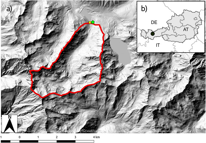
FIGURE 1. (A) Locations of the Längentalbach catchment (red outline), the gauging station (yellow triangle) and the Kühtai climate and snow monitoring stations (green pentagon). (B) overview map.

2.2 Meteorological Forcing and Evaluation Data

A snow monitoring station is situated in close proximity to the catchment outlet. This station (Kühtai, 1,920 m a.s.l.) provides recordings of the common meteorological variables air temperature, relative humidity, precipitation and incoming shortwave radiation. Measurements of snow water equivalent by a 10 m² snow pillow and snowpack runoff from an underlying lysimeter are also available. A 25-years dataset is freely available (Parajka, 2017). Recordings of wind speed and longwave irradiance are, however, not available at the Kühtai station during the years considered. We therefore utilize the 10 m wind speed product from the now-casting system INCA (Kann and Haiden, 2011) (1 km × 1 km cell size), which is based on climate model output and station observations, and accounts for acceleration and channeling of flow. For spatially distributed simulations, longwave irradiance is estimated within the model based on the other meteorological variables. For point-scale simulations, an analogous computation of longwave irradiance was performed offline. We compute snowfall and rainfall fractions based on two wet-bulb temperature thresholds between which mixed precipitation is allowed. The basin of the Längentalbach is gauged with regular updates of the appropriate rating curves, and quality checked data are available since 1981 from the Hydrographic Service Tyrol. Furthermore, available MODIS snow cover maps (250 m × 250 m cell size) (Notarnicola et al., 2013) enable additional evaluation of the catchment’s evolving areal snow cover fraction.

Apart from the Kühtai station, four additional climate stations are located near the catchment ($<$15 km, ranging from 659 to 1,999 m a.s.l.). These stations are used to pre-compute mean monthly elevation gradients of air temperature, precipitation and dew point temperatures; this strategy allows rapid regionalization of the forcing variables for the catchment domain. Even though all stations used to compute meteorological gradients are located below the altitude of the catchment outlet, the extrapolation of station measurements yields realistic values of simulated long term water balance components. Applying pre-computed mean monthly gradients results in average annual catchment precipitation of 1,346 mm/a (2001–2015) and actual evapotranspiration (Q_ET) of 127 mm/a. The difference between the two (1,219 mm/a) is close to the observed mean annual stream flow of 1,232 mm/a for the same period, strengthening confidence in the applicability of the extrapolated gradients.

In this study, we consider the 4 years (Figure 2) 2003/2004, 2005/2006, 2008/2009 and 2013/2014—each starting on 1st of September and ending on 30th of August the following year. Hereafter, we follow the short denotation of water years, e.g., 2004 for the period 2003/2004). No apparently erroneous or sparse snow pillow or lysimeter recordings are present in these years. Mean winter (Nov–Feb) air temperatures range from −5.8°C in 2006 to −2.5°C in 2014 at the Kühtai station. Spring air temperatures (Mar–Jun) range from 2.1°C in 2004 to 4.0°C in 2014. Seasonal snow water equivalent usually peaks in late March/mid April (between March 26 and April 4 in the considered years) with maximum values ranging from 271 mm in 2014 to 438 mm in 2004. Melt events in mid winter (Dec–Feb) are rare and rarely produce any outflow from the snowpack. From March 1 until peak snow water equivalent, melt events are a common characteristic of the catchment. During this period, the snowpack lost 28 mm in 2004, 45 mm in 2006, 1 mm in 2009 and 45 mm in 2014.

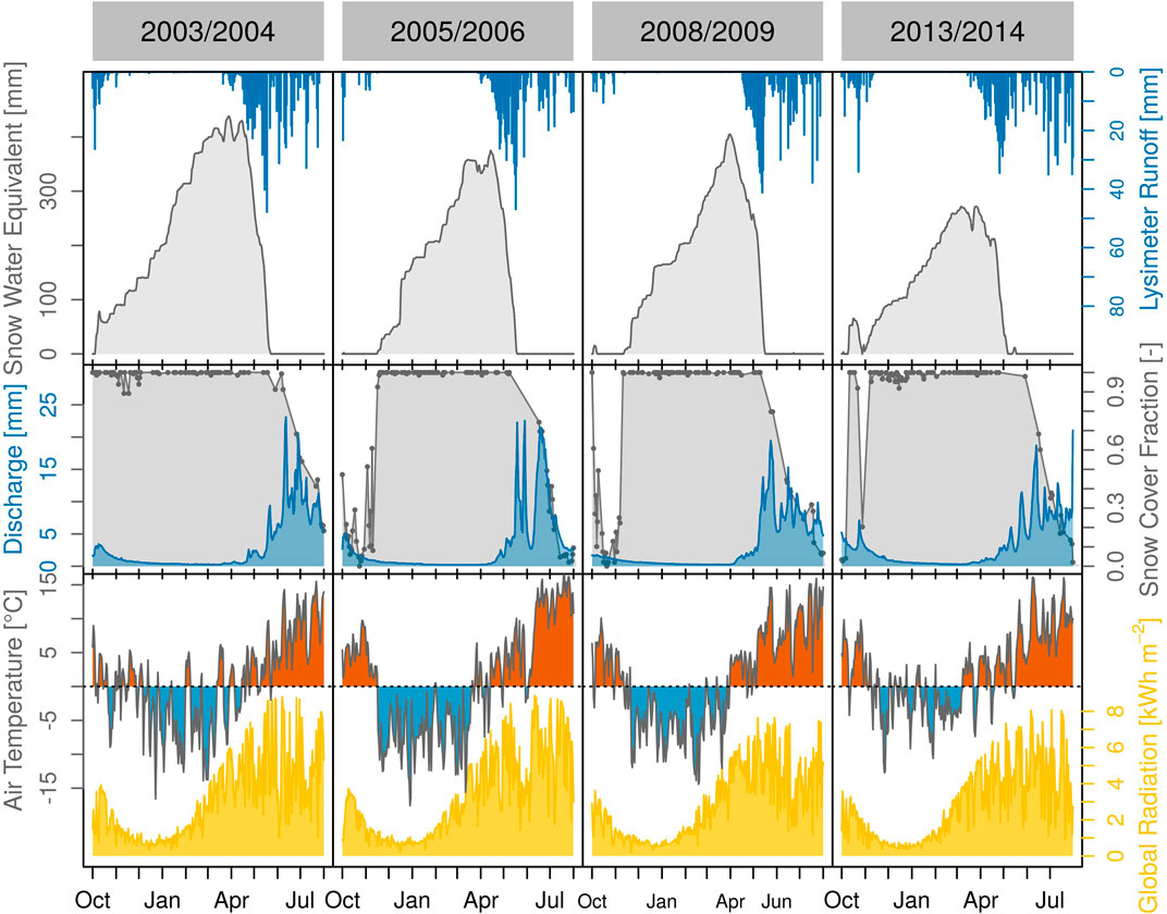
FIGURE 2. Daily recordings of snow water equivalent and lysimeter runoff (top row), MODIS snow cover fraction (cloud cover <10%) and catchment discharge (center row), and air temperature and incoming shortwave radiation (bottom row) for 4 years (columns).

2.3 Snow Model

In this study, we evaluate various process formulations commonly found in energy-balance snow models against point-scale and spatially integrated observations using the Factorial Snow Model (FSM) (Essery, 2015). FSM is a physically-based snowpack model of medium complexity that accounts for mass and energy exchanges between a maximum of three snow layers. FSM is a multi-physics model, allowing inclusion and investigation of different model structures in different simulation experiments. Five model switches for options to represent snowpack processes are available (absorption of solar radiation, heat conduction, compaction, turbulent transfer of energy, and storage of liquid water; Table 1). A simpler option (option 0) or a more complex or prognostic option (option 1) can be chosen, for each of these processes. All options can be switched on or off independently, resulting in a total of 32 distinct model structures with different degrees of complexity.

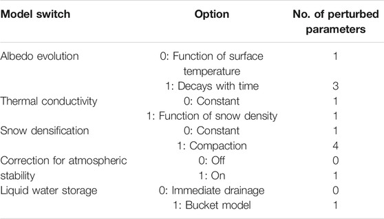
TABLE 1. Process representations available in the factorial snowpack model FSM and the number of perturbed parameters per option. The combination of these model options result in 32 different snow model structures.

Point-scale simulations are carried out by the FSM stand-alone version. For a spatially distributed application of the snow model, FSM is coupled to the framework of the hydroclimatological model AMUNDSEN (Strasser, 2008; Hanzer et al., 2016) in this study. We utilize its ability to read, process and regionalize meteorological forcings over a regular grid in complex topography, accounting for shading of terrain, preferential snow deposition, snow redistribution by wind and snow-canopy interaction. In the model, unmeasured forcing variables such as the longwave irradiance and the precipitation phase can be parameterized. In the AMUNDSEN version we use here, the coupled energy and mass-balance of the snowpack is then solved at every grid point by FSM.

2.4 Simulation Design

Due to computational restrictions, we follow a two-tier experimental design. Tier one consists of point-scale snow simulations at the monitoring station Kühtai, carried out by the 1D stand-alone version of FSM. Here, it is possible to engage in costly optimization procedures. In tier two, the spatially distributed coupled AMUNDSEN-FSM model is set up for the domain of the Längentalbach catchment (gridsize 100 m by 100 m). The spatially distributed simulations only allow a much smaller number of model evaluations. All simulations are carried out over 4 years (1st of September to 31st of August) and are based on an hourly time step. To evaluate individual model realizations out of sample, the four years are grouped into two separate periods (2004 and 2006; 2009 and 2014). Both periods are used alternately as calibration and evaluation periods.

We use the 32 combinations of process representations in FSM to mimic a suite of snow models (model structures) of different complexities. As described in Table 1, each model option is represented by an integer value of 0 or 1, with 0 being the simpler option of the two. A model structure is thus described by a five digit binary number representing the option choices for the five process representations. The sum of the binary digits gives a proxy for model complexity in an ordinal scale from 0 to 5. Complexity values are not uniformly distributed across the 32 model combinations; more model structures of medium complexity exist than simpler or more complex ones.

To include the influence of parameter uncertainty on physically-based snow simulations, all 32 model structures are configured with parameter values sampled from physically meaningful ranges. Wherever possible, these parameter ranges are taken from literature to ensure that values are typical and generally used in current snow modeling exercises (see Supplementry Table S1 for details). Depending on the FSM configuration, between 7 and 14 parameters are perturbed. Four parameters are shared by all FSM configurations, and individual options have between 3 and 10 additional parameters (Table 1; Supplementary Table 1).

2.4.1 Model Calibration

We test whether or not it is possible to reach the same performance with various complex energy balance snow models by parameter optimization. Parameter sets for all 32 model structures are optimized against snow pillow and lysimeter observations (see Section 2.5 for details of the error function) by employing a differential evolution algorithm (Price et al., 2005). 150 populations, each consisting of 70–140 members, are evaluated in the course of the calibration procedure. This results in at least 10,500 iterations per model structure. Visual inspection suggests sufficient convergence of the results.

Even for small study sites where climate station recordings are available, the generation of spatially distributed input data entails uncertainties. Analogously, we test if a comparable error minimum between different physically-based snow models can be achieved even when they are forced with heavily flawed input data at the point-scale. In this study, we utilize the forcing data described in Section 2.2 (hereafter denoted as baseline). The four forcing variables air temperature, precipitation, incoming shortwave radiation and longwave irradiance have been shown to greatly influence snow model skill (Günther et al., 2019). We therefore specify eight additional input error scenarios by applying biases one at a time to the baseline forcing, including precipitations biases of −20/+30%, air temperature biases of ±3°C, incoming shortwave biases of ±100 W m⁻² (during daytime), and longwave irradiance biases of ±25 W m⁻². These errors reproduce the 1st and 99th percentiles of the error distribution from Günther et al. (2019). In reality, errors in the forcing data may be the combined result of biases, seasonal or event-based errors, random noise or errors in the spatial extrapolation of a signal such as a gradient mismatch or special local meteorological conditions not captured in the observations. However, biases were found to have the largest influence on model performance (Raleigh et al., 2015) and are convenient to apply.

2.4.2 Model Evaluation

The model’s capability for generalization is assessed and a possible linkage to model complexity is explored by evaluating calibrated model structures out of sample. To assess temporal parameter transferability, each model structure is calibrated against point-scale observations in period 1 and evaluated in period 2 (and vice versa). Parameter transferability from point-scale simulations to spatially distributed applications is assessed by evaluating previously calibrated model structures at the catchment-scale.

To put the global error minima obtained from the optimization into the context of overall parameter uncertainty, the relationship between errors in period 1 and 2 are explored in more detail. We sample the whole parameter space with a standard latin hypercube stratified sampling technique. Each parameter is divided into bins (400 for point-scale and 20 for catchment-scale simulation), out of which samples are taken according to the overall number of parameters (resulting in 134,400 point-scale and 6,720 catchment-scale simulations). This procedure maps a large part of the parameter space onto output performance and hence enables a broader visualization of the relationship between “in sample” and “out of sample” performances.

2.5 Model Evaluation Metrics

Model simulations are evaluated against both point-scale and spatially integrated (i.e., catchment-scale) observations. Model errors are calculated with daily values for each water year. The abilities of the model to predict snow water equivalent evolution and snowpack runoff are assessed by the Kling-Gupta efficiency (Gupta et al., 2009) only during periods when a snowpack is present (either modeled or observed). These model efficiencies are transformed into the model error terms $E_{SWE}$ and $E_R$ as 1—Kling–Gupta efficiency.

The ability of the model to correctly predict the timing of snow disappearance is compared to a 250 m MODIS snow cover product for cloud free conditions (Notarnicola et al., 2013). Simulated and MODIS snow cover fraction are compared during the melt out period starting with the first decrease in simulated or observed snow cover fraction and ending with snow free conditions in 85% of the catchment area. After omitting cloud obstructed MODIS scenes, we calculate the mean absolute error of observed and simulated snow cover fraction (E_SCF).

Because this study focuses on snow modeling only, we want to avoid possible feedbacks with further abstractions of hydrological processes (e.g., water flow through the unsaturated and saturated zone, channel routing etc.). Therefore, we refrain from a classical hydrograph comparison and assess the performance of the simulations from a water balance point of view. We therefor evaluate the catchment-wide water mass temporally stored in the snowpack from the accumulation period (i.e., winter) into the depletion period (i.e., the spring freshet). Specifically, we compare the volume of observed basin discharge during the main snow melt season (i.e., starting with the first observed melt water release at the Kühtai station and ending with a snow cover lower than 15% as observed by MODIS) with the simulated water balance during this period. We calculate a percentage water balance error ($E_{WB}$) as

where it is assumed that the basin discharge (Q) equals the sum of the catchment-wide water mass drained from the snowpack (R_c) and the rainfall on snow free areas (P_rain) minus bare ground evapotranspiration (Q_ET) and storage change (ΔS) at this seasonal scale. During the frozen state of an alpine catchment, i.e., the period where all precipitation is stored in the snowpack and snowmelt is not yet occurring, observed baseflow is sustained by subsurface storage (e.g., groundwater) (Stoelzle et al., 2019). We estimate the storage change ΔS during each melt season as the cumulated volume of baseflow discharge during the catchment’s frozen state, assuming that the subsurface storage is recharged by this volume during the spring freshet. The frozen state period is identified by means of the lysimeter recordings.

Using multi-objective criteria in model selection has been shown in numerous studies (e.g., Finger et al., 2015; Hanzer et al., 2016) to reduce the risk that a correct model output is produced for the wrong reasons (Kirchner, 2006). To combine multiple objective functions within one simulation period, we calculate the combined error function as the square root of the sum of squared individual error terms. Model performance at the point-scale for the simulation period i is described by the error function

where $i1$ and $i2$ denote the first and second years of period i. Analogously, combined errors against spatially integrated observations are computed as $E_{SCF;i}=\sqrt{E_{SCF;i1}^2+E_{SCF;i2}^2}$ and $E_{WB;i}=\sqrt{E_{WB;i1}^2+E_{WB;i2}^2}$. This error aggregation penalizes model realizations that perform poorly in certain years and/or for certain objective functions. The model error over both periods is then simply given as the mean. All presented error terms imply unity at a value of 0 and increase with decreasing model skill.

3 Results

3.1 Calibrated Model Performances

We hypothesized that any model structure can have very similar performance (close to an optimum value after calibration) when parameter uncertainty is fully accounted for in physically-based snow models. To test this, all 32 model structures are calibrated against point-scale observations of snow water equivalent and snowpack runoff for the two simulation periods 2004, 2006 and 2009, 2014.

Figure 3 displays errors for all 32 model structures. Individual model structures are grouped according to their model complexity class for greater visual clarity. The boxplots represent model responses over a large part of the parameter space (as sampled from a latin hypercube of size 400 times the number of parameters). This represents the distribution of model responses when parameters are sampled randomly (but are restricted to physically meaningful values), so model errors will very likely be within this distribution if a parameter set is chosen manually without any further restricting knowledge of the system. As an example, model errors using the default parameter values for each model option are displayed as gray points. Furthermore, in order to provide context for the error values shown, the averages of all model errors are displayed as a horizontal dashed line. This represents the model skill that can be expected (in average) when parameters are chosen randomly. Blue squares show the errors of model realizations with parameters optimized by a differential evolution algorithm (i.e., parameters are specifically sampled to minimize errors). Even though minimum errors do not quite converge to a single optimal value for all models, it is evident that they are very similar, and very low error values can be achieved for all model structures and both simulation periods.

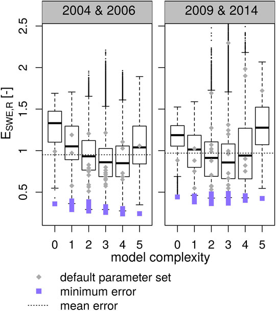
FIGURE 3. Point-scale simulation errors against snow water equivalent and snowpack runoff $\left(E_{SWE,R}\right)$ for all 32 FSM model structures and different parameter sampling techniques, grouped according to model complexity class. Boxplots encompass all model evaluations obtained from latin hypercube samples, gray points indicate model skill resulting from the default parameter set, the horizontal dotted line shows the mean error over all model realizations, and blue squares show the global error minima obtained through calibration.

“Garbage in, garbage out” is a well known phrase in computer science and mathematics, stating that the quality of output is predetermined by the quality of the input data. However, we argue that this simple relationship does not hold in snow modeling (and environmental modeling in general). The degree of equifinality in modeling systems due to uncertainty introduced by inappropriate and incomplete representations of physical properties and processes might even prevent the modeller from noticing “garbage” input.

To demonstrate this, the average model performance after parameter optimization for various input error scenarios is shown in Figure 4. Each boxplot consists of 32 data points for the 32 model structures, so a low spread in model performance (a small boxplot) would indicate that all models can indeed be calibrated close to the same value. In fact, this is observed not only for the baseline scenario, but also for a air temperature bias of −3°C and positive and negative shortwave and longwave irradiance biases to some degree. Except for the longwave error scenario, calibrated model skills are not statistically significantly different from skills obtained with baseline forcings (paired Wilcoxon signed-rank test, α = 10%). It should again be noted that each boxplot displays the calibration results of 32 different model structures, so minimum and maximum values (i.e., the ranges) are important properties. When forced with too little precipitation for example, half of the models are still able to reach a very low (i.e., <0.5) model error. All of these model structures employ a bucket model for liquid water storage in the snowpack (option 1). While no model structure is able to fully compensate for too much precipitation to a very high level of performance, it is interesting to note that analogously the better performing half of the models all drain liquid water immediately (option 0). When forced with an air temperature bias of +3°C, very good model skill (i.e., errors < 0.5) can only be achieved by the 16 model structures that utilize the correction for the atmospheric stability (option 1). For simulations with a negative bias of longwave irradiance, all model combinations with error values above 0.5 (i.e., the outliers) use the prognostic albedo option (option 1), the correction for atmospheric stability (option 1) and the liquid water storage option (option 1). When forced with a positive bias of longwave irradiance, the three worst performing models utilize the opposite options. Looking at the evaluation errors (red boxplots) reveals that even when forced with biased input data, evaluation performance can be similar to an unaltered “baseline”. For an negative air temperature bias, a negative bias of incoming shortwave radiation and a positive longwave irradiance bias evaluation performance are statistically indifferent to the baseline error scenario.

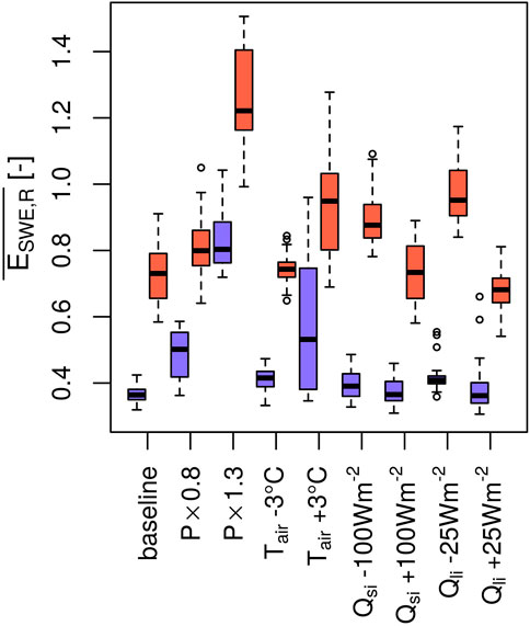
FIGURE 4. Calibration (blue boxplots) and evaluation model errors (red boxplots) for snow water equivalent and snowpack runoff, averaged over both simulation periods $\left(\overline{E_{SWE,R}}\right)$. Models are forced with unaltered input data (baseline) and eight additional error scenarios including positive and negative biases of precipitation (P), air temperature (T_air), incoming shortwave radiation (Q_si)and longwave irradiance (Q_li).

3.2 Evaluating Calibrated Model Structures at the Point Scale

We proved that all considered model structures can reach very high model skills via parameter optimization, but the level of trust one can put in a model is very much dependent on its ability to perform well out of sample, i.e., how robustly it performs in new conditions or with new data. Here, we test how well calibrated model structures can be applied in different years.

All model structures were calibrated during two years and subsequently their performance was assessed during an evaluation period of two other years. The calibration and evaluation periods were then switched and the procedure was repeated. Figure 5 shows average model errors during the calibration period and corresponding errors during the evaluation period. Calibrated model skills are very similar across the model structures (0.32–0.42) but slightly smaller for more complex models on average. The models show a much larger range in evaluation errors (0.58–0.91), but they follow the same general pattern with more complex models tending to perform better than simpler ones. The dashed line in the bottom panel indicates the maximum error of the ten best performing model structures in the evaluation period. No model of complexity classes 0 or 1 is part of this well performing sub-ensemble. However, given the variability of model errors within one complexity class, it is clear that model complexity (or our model complexity proxy) alone is not the dominating feature governing the calibration or evaluation performance, which might be more influenced by individual combinations of process options. While there is a considerable spread of evaluation performances, no model structure fails dramatically (an error value of 0.9 can be achieved by a Kling–Gupta efficiency of 0.8 for snow water equivalent and 0.4 for snowpack runoff in both years, for example). However, some models do perform better than others. Consequently, we will disentangle what separates these better performing models from the model ensemble in Section 3.4.

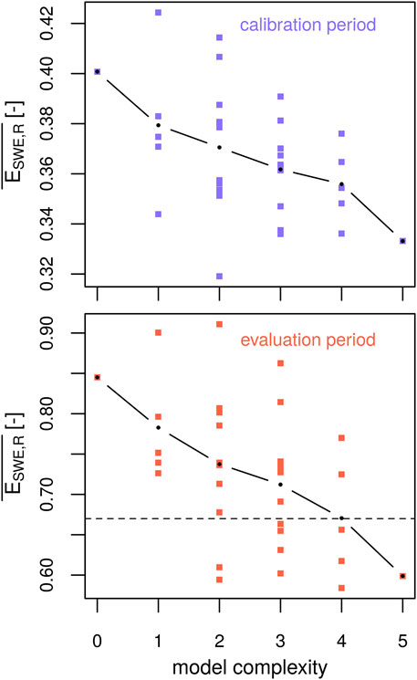
FIGURE 5. Calibration errors (upper panel) and resulting evaluation errors (lower panel) averaged over the two simulation periods for point-scale simulations of snow water equivalent and snowpack runoff $\left(\overline{E_{SWE,R}}\right)$. Models are grouped according to their complexity class and the mean of each class is indicated by the solid black line. A subset of 10 model structures with the lowest evaluation errors is located below the dashed line.

3.3 Evaluating Calibrated Model Structures at the Catchment-Scale

Another way to evaluate a model’s performance out of sample is to apply it at different locations. We expose the models to various new conditions within a spatially distributed application over the domain of the Längental and evaluate its performance integrated over the whole catchment. As described before, many considerations differ between point-scale and spatially distributed applications of snow models, e.g., about important length scales, parameter aggregation over grid elements or forcing data uncertainty. However, if a model offers a strong linkage between point-scale and catchment-scale performance, this would strengthen our trust in its robustness (i.e., in its ability to generalize).

For each model structure, parameter sets optimized against point-scale observations are applied within the spatially distributed AMUNDSEN-FSM. The snow cover in the catchment of the Längentalbach is simulated over the same period and evaluated against spatially integrated snow cover fraction and the spring water balance. In Figure 6, evaluation errors against snow cover fraction and spring water balance are shown for all 32 model structures according to their complexity class. We see a similar picture for both snow cover fraction and spring water balance compared to the point-scale evaluation errors presented in Figure 5, in that mean model errors decrease slightly with increasing model complexity, but variability within single complexity classes is substantial (e.g., complexity class 2 covers almost the whole range of errors). Evaluation errors range from 0.16 to 0.25 for snow cover fraction and from 11 to 16% for the water balance. For context, the average model error that can be expected on average, when parameters are chosen randomly is 0.35 for snow cover fraction and 17% for the spring water balance across all models. In contrast to the evaluation errors at the point-scale (Figure 5) and for snow cover fraction, where no model of class 0 or 1 is within the 10 best runs, the evaluation error against the spring water balance is lowest for one of the models of complexity class 1.

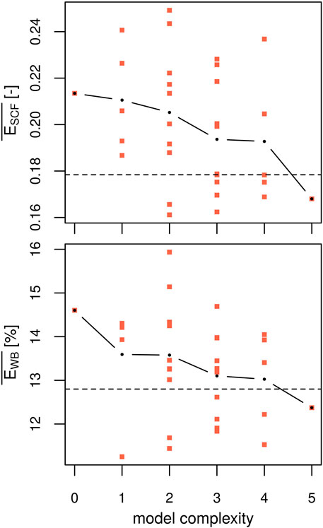
FIGURE 6. Evaluation errors of the spatially distributed simulations. Thirty two model structures are calibrated against point-scale observations of snow water equivalent and snowpack runoff and evaluated against catchment average snow cover fraction ($\overline{E_{SCF}}$; upper panel) and spring water balance ($\overline{E_{WB}}$; lower panel). Models are grouped according to their complexity class and the mean of each class is indicated by the solid black line. The 10 model structures with the lowest evaluation errors are located below the dashed line.

3.4 Can We Identify Model Structures That Perform Better Than Others?

The ten model structures that show the smallest average evaluation errors at the point and catchment-scales are selected and the options that they use are displayed in Figure 7. It is evident that there is no clear, consistent picture in terms of option usage across the three evaluation criteria, except that they do not depend very much on the thermal conductivity option used. While the option to correct for atmospheric stability seems mandatory for low evaluation errors at the point-scale (all ten runs use option 1), it has lower importance for the prediction of catchment water balance and even less so for areal snow cover fraction. In fact, only two model structures appear in all three subsets: model 7 (0,0,1,1,1) and model 31 (1,1,1,1,1).

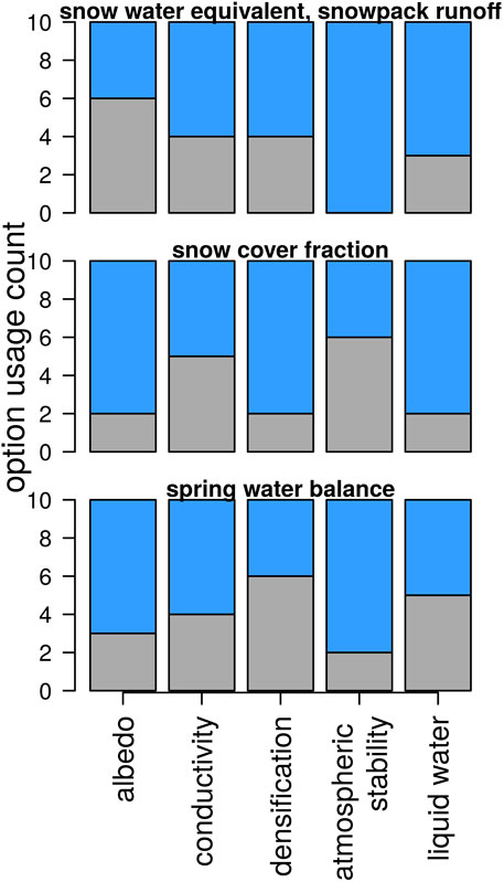
FIGURE 7. Model option occurrence (gray: option 0, blue: option 1) in the the 10 best performing model structures. Best model realizations are selected against point-scale observations of snow water equivalent and snowpack runoff (top row), catchment average snow cover fraction (center row) and spring water balance (lower row).

Evaluation performance of a previously calibrated model is a very interesting feature that allows assessment of its capability for generalization or overfitting. We acknowledge that the global error minimum within the parameter space (assuming it can be found by parameter calibration) is in some sense the only point in this space where model structures (and their responses) can be compared. However, as we argued earlier, global parameter optimization is not common in physically-based snow modeling, largely due to the notion that it is not (or at least should not be) required by these types of models, but also due to computational restrictions - even for point-scale applications of the most complex models. It is very unlikely that a global error minimum can be found when parameters are perturbed in a limited fashion around a default parameter set based on expert knowledge. Hence, considering practical limitations, the relationship between model performances across sampled parameter values can be informative for applications of such models. We therefore also sampled the model parameter space to visualize model responses over a large part of it, rather than for obtaining global minima. Parameter values were sampled by a latin hypercube (2,800–6,800 simulations per model) and the model responses for simulation periods 1 and 2 are visualized in Figure 8. Global error minima are alos indicated (red squares) for each period. Six model structures that show good performance according to the mean evaluation error (and can be found in the subset of the 10 best performing models) are presented as an example. It is evident from visual inspection that the errors for model structures 31, 27, and 19 are more strongly correlated between the simulation periods. We observe a strong correlation between all models using option 1 for albedo, atmospheric stability and liquid water storage. We acknowledge that some critical regions of the response surface remain hidden (the red squares lie outside the black circles), but model performance without calibration by downhill methods is very likely captured by the latin hypercube sample, and the density of the black circles represents a proxy for the probability of reaching a certain performance. This has implications for model intercomparison studies (of these types of snow models) where parameter sets are usually predefined. If models are compared based on the results of a single simulation, the outcome of this comparison can be manifold and will depend on the location of this simulation in the response surface. If model structures 30 and 31 are to be compared, for example, one may find that one model results in poor performance in both years and the other results in good performance in both years. However, as illustrated by the latin hypercube sample, it is also possible for model structure 30 to simultaneously show good performance in 2009/2014 and poor performance in 2004/2006, while this does not seem possible for model structure 31. Analogous graphs for all model structures can be found in the Supplementary Figure S1.

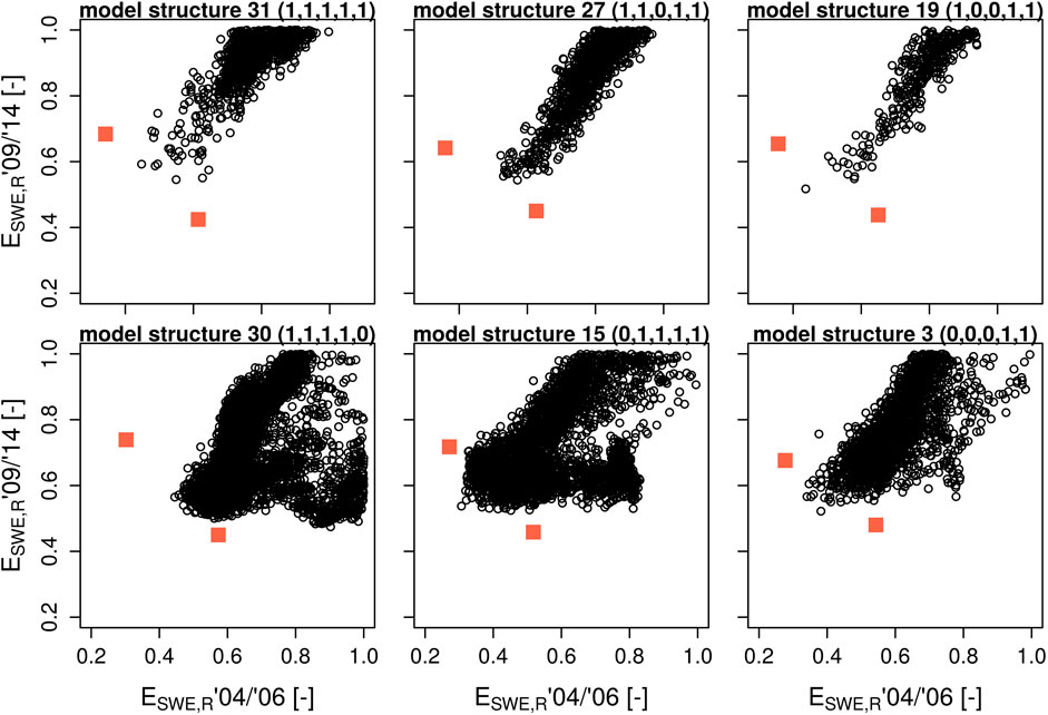
FIGURE 8. Relationships of point-scale snow water equivalent and snowpack runoff errors $\left(E_{SWE,R}\right)$ between the two simulation periods 2004/2006 and 2009/2014. Black circles are model errors for a large part of the parameter space sampled by a latin hypercube with size 400 times the number of parameters. Red squares indicate evaluation errors in one season when calibrated to minimize errors in the other season.

Concerning relationships between combined point-scale errors of snow water equivalent and snowpack runoff and catchment-scale errors of snow cover fraction and spring water balance, we can also identify specific correlation patterns and link them with individual process options (Figure 9). Computational effort for the spatially distributed application restricts the analysis to a much smaller ensemble (140–340 runs per model). When comparing mean model errors for snow water equivalent and snowpack runoff predictions with areal snow cover fraction, three basic correlation patterns emerge. All models that do not correct for atmospheric stability follow the general nonlinear pattern seen for model structure 5, where the highest model skills for point-scale simulations are associated with lower errors for snow cover fraction, but a low error in snow cover fraction does not guarantee good performance for snow water equivalent and snowpack runoff. When the atmospheric stability option is switched on but water drains immediately (storage option 0), the relationship between snow water equivalent/snowpack runoff and snow cover fraction errors shows a distinct loop-like pattern where low snow cover fraction errors can be achieved for very high snow water equivalent and snowpack runoff errors. A more linear pattern emerges when both options are switched on, especially when the albedo option is also set to 1. The same three options also prove to be relevant for determining the shape of the correlation between point-scale model errors and water balance errors. In general, the slope of the correlations tends to be positive when the atmospheric stability option is switched on (e.g., models 30 and 31) and negative when it is switched off (e.g., model 5). This correlation is stronger when the albedo option is also switched off. When water storage is enabled, it is possible to obtain low water balance errors and high point-scale errors at the same time. It is also interesting to note that all model structures that do not correct the turbulent fluxes for atmospheric stability show much smaller maximum errors for snow cover fraction and the water balance, compared to all model structures where this option is switched on. Again, analogous graphs for all model structures can be found in the Supplementary Material of this manuscript.

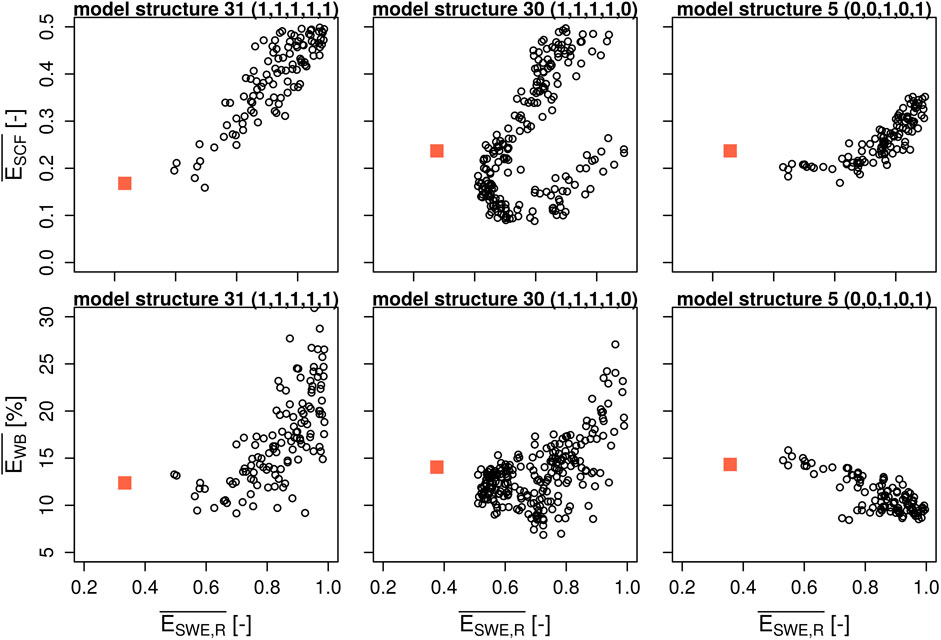
FIGURE 9. Relationship of mean model errors between point-scale snow water equivalent and snowpack runoff predictions $\left(\overline{E_{SWE,R}}\right)$ and catchment snow cover fraction ($\overline{E_{SCF}}$; top row) and catchment spring water balance ($\overline{E_{WB}}$; bottom row) for three different model structures. Black circles are model errors for a part of the parameter space sampled by a latin hypercube of size 20 times the number of parameters. Red squares indicate mean evaluation errors when parameters have been calibrated at the point-scale with a differential evolution algorithm.

4 Discussion

4.1 Parameter Uncertainty and Model Performance

We have proved that it is possible to get a variety of snow model structures close to an optimum value of an error function for snow water equivalent and snowpack runoff prediction by parameter optimization. Although the global error minimum was not as wide as previously expected for the analyzed model structures and finding it required specific sampling (i.e., calibration), this shows that there are enough degrees of freedom to do so within a physically meaningful parameter space. Some model structures might converge earlier than others, but final performances are close enough that meaningful separation of model structures becomes questionable.

We extended the analysis further and showed that this is even possible when the models are forced with considerably flawed input data. Across a range of input biases, many models were still able to reach a comparable performance optimum after calibration. Even at monitoring stations with high-end equipment and frequent visits, the quality of recorded data will always be uncertain to some degree. This holds true even more when unmeasured forcing variables have to be approximated and for spatially distributed applications in which various assumptions have to be made to extrapolate point measurements. The applied forcing biases might seem high when a model is run at the location of a climate station, but they were selected to represent a range of errors expected when observations are missing (e.g., in spatially distributed applications). The ability to compensate for erroneous forcing data is certainly not a desirable model feature, but we have shown that compensation effects do exist and can be substantial. Such compensation effects can hide even large errors in the input data (if the models are not evaluated out of sample). Surprisingly, even higher performances can be achieved with deliberately modified input data after calibration for some model options because they favor the compensation of specific forcing errors. Our results confirm an increase in model performance variability only for some error scenarios (as illustrated in Figure 4).

Comparing models based on their performance out of sample, as is common for conceptual models, is a more promising endeavor. This is of course well recognized, and in recent snow model intercomparison studies (Krinner et al., 2018) several snow models have been compared at different locations with very different climatic characteristics (and consequently differing importance of processes), while preventing parameter optimization by withholding evaluation data sets. In this work, we perturbed parameters over a whole range of physically meaningful values to highlight that parameter uncertainty can compensate structural deficiencies for physically-based snow models. However, if parameter uncertainty is reduced (e.g., by fixing or reducing the ranges of the measured parameters), we also expect that differences in model structures will become more visible in the results. Still, the point that there will be compensation effects to some degree remains valid. Consequently, this study shows that model intercomparisons in the face of parameter uncertainty should ideally not be based on comparing single, uncalibrated model realizations even for physically-based snow models, and the impact of parameter uncertainty should be considered. A comparison strategy based on an ensemble of simulations could be a way forward.

4.2 The Role of Model Complexity

Previous model comparison studies have found that model complexity above a certain minimum is required for good results, but a higher model complexity does not necessarily increase model performance (Essery et al., 2013; Magnusson et al., 2015). In this study, we extend their analyses by including parameter uncertainty and compare performances of previously calibrated models. Our results confirm the findings in that simpler models (of class 0 and 1) can be found less frequently in a group of well performing simulations when evaluated out of sample, and models of higher complexity do perform better more frequently. The highest model complexity, represented by model structure 31, does not show the highest model performance for every evaluation criterion. Less complex models often achieve better results. However, model structure 31 is found along with model structure 7 (complexity class 3) in all well performing subsets.

Furthermore, a model of higher complexity does not always produce good or even acceptable results, even when parameters are just perturbed within a physical meaningful space. When looking at the whole model ensemble for the baseline input scenario, we can find model realizations for each complexity class resulting in unsatisfactory model performance (E_SWE,E > 1.5, E_SCF > 0.4, and E_WB > 30%). In fact, the highest errors can be achieved by the more complex models. Model realizations using the options for the atmospheric stability correction and water storage in snow can produce high error values. When air temperature is higher than the snow surface temperature, the atmospheric stability option limits the transfer of energy to the snow surface from the lower atmosphere, which can delay modeled snowmelt for stable conditions. When this option is switched off, stratification is neglected and there is no effective limitation of the turbulent fluxes in stable conditions. Surface temperature then reacts much faster to air temperature signals. Liquid water storage inside the snowpack (option 1) allows for refreezing of liquid water, e.g., during nighttime. For sites with a strong diurnal cycle of energy input, or with very deep snowpacks, this refreezing might be crucial for their mass balance. However, large snow masses can build up and melt can be delayed when refreezing is not parameterized correctly. Although the combination of both options can lead to large errors for snow water equivalent/snowpack runoff, snow cover fraction and spring water balance, this combination can also be commonly found in the subsets of the 10 best performing models. Interestingly, all models that are never found in any of the three 10 best model subsets do not utilize both options together. This emphasizes that model complexity (or at least the complexity proxy used here) is not sufficient to predict well performing model structures. As each of the complexity classes 1–4 include multiple model structures, they also include both options for every process representation.

While the focus of this study lies on the intercomparion of energy-balance snow models, for context we provide the results of an analogous analysis for a simple temperature index (t-index) snow model. The t-index model, consisting of an air temperature threshold value and a varying air temperature-based snow melt factor for early season and late season, is run at a daily time-step. We found that for point-scale simulations of snow water equivalent and snowpack runoff the t-index model did not lead to lower error values as its physically-based counterparts, neither in the calibration nor in the evaluation period ($\overline{E_{SWE,R}}$ = 0.7 and 1.05, respectively). However, as suggested by Seibert et al. (2018) for benchmarking hydrological models, when run with randomly chosen parameter-sets (n = 1,000), the average time-series of the resulting t-index ensemble performs surprisingly well ($\overline{E_{SWE,R}}$ = 0.95). In fact, for snow cover fraction this ensemble average performs better than most individual realizations of the physically-based models ($\overline{E_{SCF}}$ = 0.13). Simpler models (or model options) are usually computationally cheaper, and hence, facilitate the use of ensemble-based methods (e.g., in operational applications). Hence, future snow model intercomparison studies could allow model output aggregation (e.g., ensemble statistics) for simpler models and explore their benefits in more detail.

4.3 Which Process Options are Used by Well Performing Models?

What is a good model might depend upon the specific application of the model, e.g., for certain types of melt events, large domain simulations or individual (critical) events (Bennett et al., 2013). In this study, we asses model performance for the combined prediction of point-scale snow water equivalent and snowpack runoff, and catchment-wide snow cover fraction and water balance over multiple seasons. Evaluating previously calibrated model structures in time (during different seasons) and space (in a spatially distributed application) did not reveal many consistent results other than that the choice of model structures 7 (0,0,1,1,1) or 31 (1,1,1,1,1) yield good evaluation results for all error criteria. The visualization of model responses across a sample of the parameter space (Figures 8 and 9) allowed the exploration of model behavior beyond the singular relation of calibration-evaluation performance. In this study, we did not present a methodology to analyze the resulting correlation pattern rigorously. To be robust, the development of such a strategy would be best done at multiple sites with quality-checked forcing and evaluation data, and where parameter uncertainty can be reduced by observations. Instead, we primarily want to show that there are distinct differences between model structures which remain hidden if only single (calibrated or uncalibrated) model realizations are evaluated. In our case, the response surfaces identified that all four model structures that utilize the prognostic option for albedo decay, correction of turbulent fluxes for atmospheric stability and liquid water storage in snow (1,x,x,1,1) offer a more distinct correlation between the two simulation periods and between snow water equivalent/snowpack runoff and areal snow cover fraction errors, and at least do not have negative correlations between snow water equivalent/snowpack runoff and water balance errors. Again, how robust these findings are for other seasons and different climates remains to be assessed in future studies.

4.4 What Prevents us From Obtaining More Consistent Results?

In our analysis of a large snow model ensemble, consistent findings across different performance metrics are rare. Optimum model performance values achieved through calibration are all below unity, with errors being slightly smaller for period 1 (2004/2006) compared to period 2 (2009/2014). Optimal skill values are not just governed by deficiencies in the model setup (i.e., model structure and parameter values), but also further degraded by input and evaluation data quality. How much these individual components contribute to the degradation of the optimum value remains unknown, but it is clear that the forcing and evaluation data might play a major role for the analyzed dataset. Some of the required inputs are not directly observed and need to be approximated (precipitation phase, longwave irradiance, wind speed; see Section 2.2). Also, there might be erroneous recordings in the evaluation data. It is possible that our “baseline” forcing scenario includes enough uncertainty that findings might differ substantially when models are forced with perfect (or better) data. An implicitly accepted forcing (or evaluation) data error during the calibration phase might have nonlinear consequences. There might be model structures that are not sensitive to a specific kind of error or even profit from such errors as they can compensate some of their structural uncertainty. Indeed, we showed that some model options can compensate specific forcing biases better than others for the calibration period. Extending the analysis to better equipped climate stations could be a valuable test, as the correlated uncertainties of forcing data, model structure and parameter choice could be reduced.

Assessing a model’s ability to predict a certain output by condensing the deviations between a simulation and observations to a single performance measure is always a difficult task, as different performance metrics are sensitive to different kind of errors. It also introduces equifinality in the evaluation, as identical performance values can often be achieved by different errors (e.g., over- and underestimation of a variable can lead to the same Kling-Gupta efficiency value). This is especially obvious when time series (e.g., snow seasons) are compared. Just as different errors in the accumulation and ablation season can lead to the same skill values for individual years, combining evaluation results over multiple seasons can yield the same values for a whole range of single year performances. Aggregating results further into multi-objective performance metrics results in the same kind of equifinality. Lafaysse et al. (2017) illustrated equifinality in snow model simulations by comparing two different model structures. The authors showed that very different contributions of energy fluxes to the energy balance can result in very similar evaluation results and highlighted that this increases the difficulty of selecting a best model.

5 Conclusions

Previous studies have already investigated performances of different snow model structures within multi-physics model frameworks (Essery et al., 2013; Magnusson et al., 2015; Lafaysse et al., 2017). However, parameter uncertainty was not addressed in any of these analyses. As shown by Günther et al. (2019), the uncertainty introduced by parameter choices substantially contributes to variability in simulation accuracy.

In this study, we demonstrate that the influence of parameter uncertainty is substantial even for physically-based snow models. Due to parameter uncertainty, no model structure guarantees sufficient model performance, and care should be taken when selecting appropriate parameter values. When sampling parameters from a physically meaningful parameter space, models of different structures and various degrees of complexity all reached similar good performance values. We further showed that this is even possible (to some degree) when forcings are biased. This indicates that parameter uncertainty has a substantial capability to compensate for input errors. This compensation can even hide large errors and could potentially lead to good results for the wrong reasons.

We acknowledge that there are conflicting schools of thought about how to derive parameters for physically-based models - e.g., various types of modellers have been outlined by Pappenberger and Beven (2006) according to their willingness to accept uncertainty analysis and parameter calibration. However, we argue that for energy-balance snow models of medium complexity (as represented by the multi-physics model used here) a categorical rejection of parameter optimization or perturbation is untenable, given the degree of conceptualization with which physical processes are represented in parts. Consequently, we argue that future intercomparisons of physically-based snow models need to consider this in their design. Evaluation of previously calibrated models against point-scale observations of snow water equivalent and snowpack runoff, areal snow cover fraction and catchment spring water balance did not yield many consistent results. Only two model structures could be found within subsets of the 10 best performing models for all three evaluation metrics (structures 31 and 7). We further reason that, instead of comparing model responses for single realizations (as has been done in the previously stated studies), comparison of model ensembles covering possible parameter values (which might be further restricted by measurements) could be a way forward. Analyzing relationships in model responses between different outputs (e.g., between different seasons, during different kinds of melt events, or between different state variables) while considering parameter uncertainty (e.g., through ensemble simulations) might offer a possibility to compare across model structures in a more comprehensive way. However, such a robust methodology is yet to be developed for this. We have merely introduced the idea and shown exemplary results for our dataset.

Data Availability Statement

The datasets generated for this study are available on request to the corresponding author.

Author Contributions

DG and RE conceived the original idea. RE provided technical insights into the multi-physics snow model. FH helped with developing the computational framework and the set up on a high performance cluster. DG performed model simulation and evaluation and prepared all analysis. DG wrote the manuscript with support from all co-authors. US supervised the project.

Funding

This work was supported by the EUREGIO research project CRYOMON-SciPro FIPN000100. Development of FSM is supported by NERC Grant NE/P011926/1. Publication of the manuscript is gratefully supported by the University of Innsbruck. The computational results presented were achieved in part using the Vienna Scientific Cluster (VSC).

Conflict of Interest

The authors declare that the research was conducted in the absence of any commercial or financial relationships that could be construed as a potential conflict of interest.

Supplementary Material

The Supplementary Material for this article can be found online at: https://www.frontiersin.org/articles/10.3389/feart.2020.542599/full#supplementary-material

References

Barnett, T. P., Adam, J. C., and Lettenmaier, D. P. (2005). Potential impacts of a warming climate on water availability in snow-dominated regions. Nature 438, 303–309. doi:10.1038/nature04141
Bartelt, P., and Lehning, M. (2002). A physical SNOWPACK model for the Swiss avalanche warning: Part I: numerical model. Cold Reg. Sci. Technol. 35, 123–145. doi:10.1016/S0165-232X(02)00074-5
Beniston, M. (2012). Is snow in the Alps receding or disappearing? WIREs Clim. Change 3, 349–358. doi:10.1002/wcc.179
Bennett, N. D., Croke, B. F. W., Guariso, G., Guillaume, J. H. A., Hamilton, S. H., Jakeman, A. J., et al. (2013). Characterising performance of environmental models. Environ. Model. Softw. 40, 1–20. doi:10.1016/J.ENVSOFT.2012.09.011
Beven, K. (2012). Rainfall-runoff modelling: the primer. 2nd Edn. Chichester, United Kingdom: John Wiley and Sons. doi:10.1002/9781119951001
De Gregorio, L., Günther, D., Callegari, M., Strasser, U., Zebisch, M., Bruzzone, L., et al. 2019). Improving SWE estimation by fusion of snow models with topographic and remotely sensed data. Remote Sens. 11, 2033. doi:10.3390/rs11172033
Endrizzi, S., Gruber, S., Dall’Amico, M., and Rigon, R. (2014). GEOtop 2.0: simulating the combined energy and water balance at and below the land surface accounting for soil freezing, snow cover and terrain effects. Geosci. Model Dev. 7, 2831–2857. doi:10.5194/gmd-7-2831-2014
Essery, R. (2015). A factorial snowpack model (FSM 1.0). Geosci. Model Dev. 8, 3867–3876. doi:10.5194/gmd-8-3867-2015
Essery, R., Morin, S., Lejeune, Y., and B Ménard, C. (2013). A comparison of 1701 snow models using observations from an alpine site. Adv. Water Resour. 55, 131–148. doi:10.1016/j.advwatres.2012.07.013
Finger, D., Vis, M., Huss, M., and Seibert, J. (2015). The value of multiple data set calibration versus model complexity for improving the performance of hydrological models in mountain catchments. Water Resour. Res. 51, 1939–1958. doi:10.1002/2014WR015712
Günther, D., Marke, T., Essery, R., and Strasser, U. (2019). Uncertainties in snowpack simulations―assessing the impact of model structure, parameter choice, and forcing data error on point-scale energy balance snow model performance. Water Resour. Res. 55, 2779–2800. doi:10.1029/2018WR023403
Geitner, C., Mergili, M., Lammel, J., Moran, A., Oberparleitner, C., Meißl, G., et al. (2009). “Modelling peak runoff in small Alpine catchments based on area properties and system status.” in Sustainable natural hazard management in alpine environments. Berlin, Heidelberg: Springer, Vol. 5, 103–134. doi:10.1007/978-3-642-03229-5
Gupta, H. V., Kling, H., Yilmaz, K. K., and Martinez, G. F. (2009). Decomposition of the mean squared error and NSE performance criteria: implications for improving hydrological modelling. J. Hydrol. 377, 80–91. doi:10.1016/j.jhydrol.2009.08.003
Hamlet, A. F., and Lettenmaier, D. P. (2007). Effects of 20th century warming and climate variability on flood risk in the western U.S. Water Resour. Res. 43, 14–19. doi:10.1029/2006WR005099
Hanzer, F., Helfricht, K., Marke, T., and Strasser, U. (2016). Multilevel spatiotemporal validation of snow/ice mass balance and runoff modeling in glacierized catchments. Cryosphere 10, 1859–1881. doi:10.5194/tc-10-1859-2016
Kann, A., and Haiden, T. (2011). INCA—an operational nowcasting system for hydrology and other applications and other applications. Berichte Geol. B.-A. 88, 7–16.
Kirchner, J. W. (2006). Getting the right answers for the right reasons: linking measurements, analyses, and models to advance the science of hydrology. Water Resour. Res. 42, W03S04. doi:10.1029/2005WR004362
Krinner, G., Derksen, C., Essery, R., Flanner, M., Hagemann, S., Clark, M., et al. (2018). ESM-SnowMIP: assessing snow models and quantifying snow-related climate feedbacks. Geosci. Model Dev. 11, 5027–5049. doi:10.5194/gmd-11-5027-2018
Kumar, M., Marks, D., Dozier, J., Reba, M., and Winstral, A. (2013). Evaluation of distributed hydrologic impacts of temperature-index and energy-based snow models. Adv. Water Resour. 56, 77–89. doi:10.1016/j.advwatres.2013.03.006
Lafaysse, M., Cluzet, B., Dumont, M., Lejeune, Y., Vionnet, V., and Morin, S. (2017). A multiphysical ensemble system of numerical snow modelling. Cryosphere 11, 1173–1198. doi:10.5194/tc-11-1173-2017
Lehning, M., Völksch, I., Gustafsson, D., Nguyen, T. A., Stähli, M., and Zappa, M. (2006). ALPINE3D: a detailed model of mountain surface processes and its application to snow hydrology. Hydrol. Process. 20, 2111–2128. doi:10.1002/hyp.6204
Liston, G. E., and Elder, K. (2006). A distributed snow-evolution modeling system (SnowModel). J. Hydrometeorol. 7, 1259–1276. doi:10.1175/JHM548.1
Magnusson, J., Wever, N., Essery, R., Helbig, N., Winstral, A., and Jonas, T. (2015). Evaluating snow models with varying process representations for hydrological applications. Water Resour. Res. 51, 2707–2723. doi:10.1002/2014WR016498
Marks, D., Domingo, J., Susong, D., and Link, T., and Garen, D. (1999). A spatially distributed energy balance snowmelt model for application in mountain basins. Hydrol. Process. 13, 1935–1959. doi:10.1002/(sici)1099-1085(199909)13:12/13<003C1935::aid-hyp868>3.0.co;2-c
Meißl, G., Formayer, H., Klebinder, K., Kerl, F., Schöberl, F., Geitner, C., et al. (2017). Climate change effects on hydrological system conditions influencing generation of storm runoff in small Alpine catchments. Hydrol. Process. 31, 1314–1330. doi:10.1002/hyp.11104
Mosier, T. M., Hill, D. F., and Sharp, K. V. (2016). How much cryosphere model complexity is just right? exploration using the conceptual cryosphere hydrology framework. Cryosphere 10, 2147–2171. doi:10.5194/tc-10-2147-2016
Notarnicola, C., Duguay, M., Moelg, N., Schellenberger, T., Tetzlaff, A., Monsorno, R., et al. (2013). Snow cover maps from MODIS images at 250 m resolution, part 1: algorithm description. Remote Sens. 5, 110–126. doi:10.3390/rs5010110
Pappenberger, F., and Beven, K. J. (2006). Ignorance is bliss: or seven reasons not to use uncertainty analysis. Water Resour. Res. 42, W05302. doi:10.1029/2005WR004820
Parajka, J. (2017). The Kühtai dataset: 25 years of lysimetric, snow pillow and meteorological measurements. Water Resour. Res. 53, 5158–5165. doi:10.5281/ZENODO.556110
Price, K. V., Storn, R. M., and Lampinen, J. A. (2005). Differential evolution: a practical approach to global optimization. Berlin, Germany: Springer.
Raleigh, M. S., Lundquist, J. D., and Clark, M. P. (2015). Exploring the impact of forcing error characteristics on physically based snow simulations within a global sensitivity analysis framework. Hydrol. Earth Syst. Sci. 19, 3153–3179. doi:10.5194/hess-19-3153-2015
Seibert, J. (2000). Multi-criteria calibration of a conceptual runoff model using a genetic algorithm. Hydrol. Earth Syst. Sci. 4, 215–224. doi:10.5194/hess-4-215-2000
Seibert, J., Vis, M., Lewis, E., and van Meerveld, H. J. (2018). Upper and lower benchmarks in hydrological modelling. Hydrol. Process. 32, 1120–1125. doi:10.1002/hyp.11476
Stoelzle, M., Schuetz, T., Weiler, M., Stahl, K., and Tallaksen, L. M. (2019). Beyond binary baseflow separation: a delayed-flow index as a fresh perspective on streamflow contributions. Hydrol. Earth Syst. Sci. Discuss. 1, 30. doi:10.5194/hess-2019-236
Strasser, U. (2008). Tech. Rep. 55. Modelling of the mountain snow cover in the Berchtesgaden National Park.
Sun, N., Yan, H., Wigmosta, M. S., Leung, L. R., Skaggs, R., and Hou, Z. (2019). Regional snow parameters estimation for large‐domain hydrological applications in the Western United States. J. Geophys. Res. Atmos. 124, 5296–5313. doi:10.1029/2018JD030140
Vionnet, V., Brun, E., Morin, S., Boone, A., Faroux, S., Le Moigne, P., et al. (2012). The detailed snowpack scheme Crocus and its implementation in SURFEX v7.2. Geosci. Model Dev. 5, 773–791. doi:10.5194/gmd-5-773-2012
Keywords: energy balance snow modelling, multi-physics model, parameter uncertainty, parameter calibration, model complexity
Citation: Günther D, Hanzer F, Warscher M, Essery R and Strasser U (2020) Including Parameter Uncertainty in an Intercomparison of Physically-Based Snow Models. Front. Earth Sci. 8:542599. doi: 10.3389/feart.2020.542599
Received: 13 March 2020; Accepted: 05 October 2020;
Published: 28 October 2020.
Edited by:
Matthias Huss, ETH Zürich, SwitzerlandReviewed by:
Jan Seibert, University of Zurich, SwitzerlandThomas Mosier, Idaho National Laboratory (DOE), United States
Copyright © 2020 Günther, Hanzer, Warscher, Essery and Strasser. This is an open-access article distributed under the terms of the Creative Commons Attribution License (CC BY). The use, distribution or reproduction in other forums is permitted, provided the original author(s) and the copyright owner(s) are credited and that the original publication in this journal is cited, in accordance with accepted academic practice. No use, distribution or reproduction is permitted which does not comply with these terms.
*Correspondence: Daniel Günther, daniel.guenther@uibk.ac.at