Detecting Optimal Leak Locations Using Homotopy Analysis Method for Isothermal Hydrogen-Natural Gas Mixture in an Inclined Pipeline

1
Department of Mathematical Sciences, Universiti Teknologi Malaysia, Johor Bahru 81310, Malaysia
2
Department of Mathematics, Universitas Airlangga, Surabaya 60115, Indonesia
*
Author to whom correspondence should be addressed.
Symmetry 2020, 12(11), 1769; https://doi.org/10.3390/sym12111769
Submission received: 18 August 2020
/
Revised: 25 September 2020
/
Accepted: 29 September 2020
/
Published: 26 October 2020
(This article belongs to the Special Issue Integral Equations: Theories, Approximations and Applications)
Abstract
:The aim of this article is to use the Homotopy Analysis Method (HAM) to pinpoint the optimal location of leakage in an inclined pipeline containing hydrogen-natural gas mixture by obtaining quick and accurate analytical solutions for nonlinear transportation equations. The homotopy analysis method utilizes a simple and powerful technique to adjust and control the convergence region of the infinite series solution using auxiliary parameters. The auxiliary parameters provide a convenient way of controlling the convergent region of series solutions. Numerical solutions obtained by HAM indicate that the approach is highly accurate, computationally very attractive and easy to implement. The solutions obtained with HAM have been shown to be in good agreement with those obtained using the method of characteristics (MOC) and the reduced order modelling (ROM) technique.
1. Introduction
One of the strategies to reduce gas transportation costs is the use of natural gas pipeline networks by petroleum companies [1]. These networks are capable of supplying gas in long distances under high pressure and through compression stations [2]. Changes in pipeline pressure are a function of gas velocity, valve closure time, and arrangement of the closing valve [3].
When the valve is closed at the end of the pipeline, there is the possibility of the occurrence of maximum pressure, which can be decreased in short times during its closure. It is of utmost importance to control factors affecting transient pressure, such as initial pressure and mass ratio. This is because the damage caused by this pressure is not evident shortly after the event [4,5,6].
Several studies have been conducted on transient flow in the mixtures of hydrogen and natural gas with the use of isothermal flow and horizontal pipelines, which is not the case in reality [2,7,8,9]. Furthermore, another study has made an attempt to study the flow of these mixtures under high pressure through inclined pipelines [10]. In most pipelines working under high pressure, there are slow and fast fluid transients. As gas properties are not constant, a one-dimensional and non-isothermal gas flow model should be presented to simulate these transients [2].
The reason for proposing hydrogen and natural gas mixtures is their transportation through the same pipelines for the purpose of cost reduction. This is while the existing lines are just designed for natural gas, whose properties are significantly different from that of hydrogen [11,12]. The solution to this problem has been the mixture of the both with a great deal of care and attention, as hydrogen is a reactive gas with high pressure that can cause leakage [13,14]. This problem is of great importance since leakage can cause many economic, environmental, and safety problems and threaten industries and citizens by wasting natural gas [14].
According to the reports, two thirds of the 375 pipeline events between 1994 and 1999 were caused by leakage [4]. In addition, high-pressure wave celerity causes pipe splitting, and even, exploding, sometimes making intense holes that lead to inward collapse of pipes, necessitating the careful study of pressure wave celerity.
Studies have been done on leakage and its location for natural gas [15,16], leading to the introduction of methods [17,18], such as the acoustic method (AM) [18,19] and the negative pressure wave method (NPW) [20,21]. Means of transients and using unsteady-state tests, which give rise to small overpressure, can be considered as an appropriate method for detecting leaks locations in pressurised pipes [22]. Autocorrelation analysis of vibro-acoustic signals measured in a test field and amplitude distortion of measured leak noise signals caused by instrumentation have been used for water leak detection in [23,24]. In water-filled small-diameter polyethylene pipes by means of acoustic Emission Measurements, [25] has been used for detecting leak locations. However, there is paucity of research on this issue for hydrogen or its mixture with natural gas [15,16]. In this regard, isothermal and non-isothermal flow models have been proposed for hydrogen and natural gas mixtures [7,8,14].
There have been several studies on the detection of leakage location through novel approaches. For example, new leakage detection using AM [26] and new algorithm based on the attenuation of NPW in isothermal cases have been introduced in recent years [27].
Accordingly, the present study made an attempt to determine leakage location in an inclined pipe for isothermal flow containing hydrogen-natural gas mixture with the use of homotpy analysis method. This method is used for solving the governing equations, leading to quick and accurate analytical solutions for nonlinear transportation equations. Factors affecting pressure and celerity waves in inclined pipes, such as inclination angles and mass ratio of mixtures, have also been discussed. The obtained results are in good agreement for isothermal flow in a horizontal pipeline. Results showed that pressure drop and leak discharge are increased with an increase in the inclination angle, while the celerity wave and the leak location do not seem to be affected.
2. Mathematical Formulation
Figure 1 shows an inclined pipeline, which has a reservoir at the top and a valve at its bottom. The governing equations consist of three partial differential equations that are all coupled, non-linear and hyperbolic. The non-isothermal flow in the pipeline, a homogenous mixture of hydrogen and natural gas, was considered to be one-dimensional that is compressible and covers transient condition [7].
2.1. Governing Equation
The governing equations for the transport of hydrogen/natural gas mixture in an inclined pipeline from the principle of conserving mass and momentum are given by the following,
with , , is density, u is the gas velocity, P is the pressure, e is the gas internal energy per unit mass, D is the diameter of the pipeline, f is the coefficient of friction, g is the gravitational force and is an angle between the friction force and the direction.
Boundary conditions of this equations depend on the types of closure and the valve operational time. The boundary conditions at the initial point and at the end point , respectively are given by,
where and are defined as density and gas velocity at the inlet pipeline, respectively and and are defined as density and gas velocity at the outlet pipeline, respectively. The initial conditions that are assumed to be in a steady state condition at are [7],
The commonly used equation of state for perfect gas is as follows:
where,
- R: is the specific gas constant.
- T: is temperature.
The equation of state for the compressible flow, where there is a celerity pressure wave, is:
The following equations are also achieved from ideal gas relation,
where,
- : is the specific heat at constant volume.
- : is the specific heat at constant pressure.
- R: is the specific gas constant.
- P: is pressure.
- : is the flow process index.
2.2. Hydrogen-Natural Gas Mixture Equation
The mass ratio and the density of hydrogen-natural gas mixture are defined as,
with , , and . Where , , and are defined as the mass of natural gas and hydrogen and volume of natural gas and hydrogen, respectively.
Therefore, the expression of the average density of the gas mixture is given by,
3. Homotopy Analysis Method
A brief description of the standard homotopy analysis method (HAM) presented by [28,29,30,31,32]. This will be followed by a description of the algorithm of the homotopy analysis method (HAM). First, we consider the following differential equation,
where are nonlinear operators, x and t denotes the independent variable, are unknown functions, and are known analytic functions. For , Equation (14) reduces to the homogeneous equation. By means of generalizing the traditional homotopy method, Liao [28] constructed the so-called zero-order deformation equation,
where is an embedding parameter, ℏ are nonzero auxiliary functions, is an auxiliary linear operator, are initial guesses of , denotes a nonzero auxiliary function and are unknown functions. It is important to note that one has great freedom to choose auxiliary objects such as ℏ and in HAM. Obviously, when and , Equation (15) becomes,
Thus, as q increases from 0 to 1, the solution varies from the initial guesses to the solutions . Expanding in Taylor series with respect to q, one has
where,
If the auxiliary linear operator, the initial guesses, the auxiliary parameters ℏ, and the auxiliary functions are so properly chosen, then series Equation (17) converges at , and one has,
which must be one of the solutions of the original nonlinear equations, as proved by Liao [28]. As and , Equation (15) becomes,
which is used mostly in the homotopy perturbation method. Define the vectors,
Differentiate the zeroth-order deformation Equation (14) m-times with respect to q and then dividing them by and finally setting , we get the following mth-order deformation equation,
where,
with,
It should be noted that the linear Equation (22), which has linear boundary conditions, governs for [33]. Boundary conditions stem from the main problem, the solution for which can be provided by Matlab, Maple, or Mathematica. The requirement for the limit of Equation (17) is that it should meet the conditions of the main equation when it is convergent at . It is noteworthy that drawing “ℏ-curves” or “curves for convergence-control parameter” aim to find a proper convergence-control parameter ℏ, a convergent series solution, or and accelerate its convergence rate. It is such that these curves with unknown quantities are drawn against ℏ to approximately find the convergence region, though they are just graphical. This is because it is not possible to find which provides the fastest convergent series (see Liao [28,34] for further reading). Another note to be made is that a unique solution is achieved when Equation (14) accepts a unique solution; otherwise, many possible solutions will be obtained from HAM.
3.1. Solving the Steady State Equations by High-Order Deformation HAM
We define the vectors,
Differentiating Equations (5) and (6) m times with respect to the embedding parameter q and then setting and finally dividing them by , we have the so-called mth-order deformation equations,
with the initial conditions,
where,
with the celerity pressure wave defined as follows,
with the following linear operators,
with the property that,
which implies that,
Now, the solution of the mth-order deformation Equations (5) and (6) becomes,
which can be easily solved by a symbolic computation software such as Matlab, Maple, and Mathematica. Therefore, we will have and as follows,
Furthermore, to construct the zeroth-order deformation equations we can define the nonlinear operators and as follows,
with the celerity pressure wave c defined as follows,
3.2. Solving Isothermal Flow of Hydrogen-Natural Gas Mixture by HAM
We define the vectors,
Differentiating Equations (1) and (2) m times with respect to the embedding parameter q and then setting and finally dividing them by , we have the so-called mth-order deformation equations,
with the initial and boundary conditions as follows,
where,
with the celerity pressure wave defined as follows,
with the following linear operators,
with the property that,
which implies that,
Now, the solution of the mth-order deformation Equations (1) and (2) becomes,
which can be easily solved by a symbolic computation software such as Matlab, Maple, and Mathematica. Therefore, we will have and as follows,
Furthermore, to construct the zeroth-order deformation equations we can define the nonlinear operators and as follows,
with the celerity pressure wave c defined as follows,
3.3. Results and Discussion
For solving the Equations (5) and (6) by suing the homotopy analysis method according the Equations (25)–(36) we can have,
therefore, pressure is as follows,
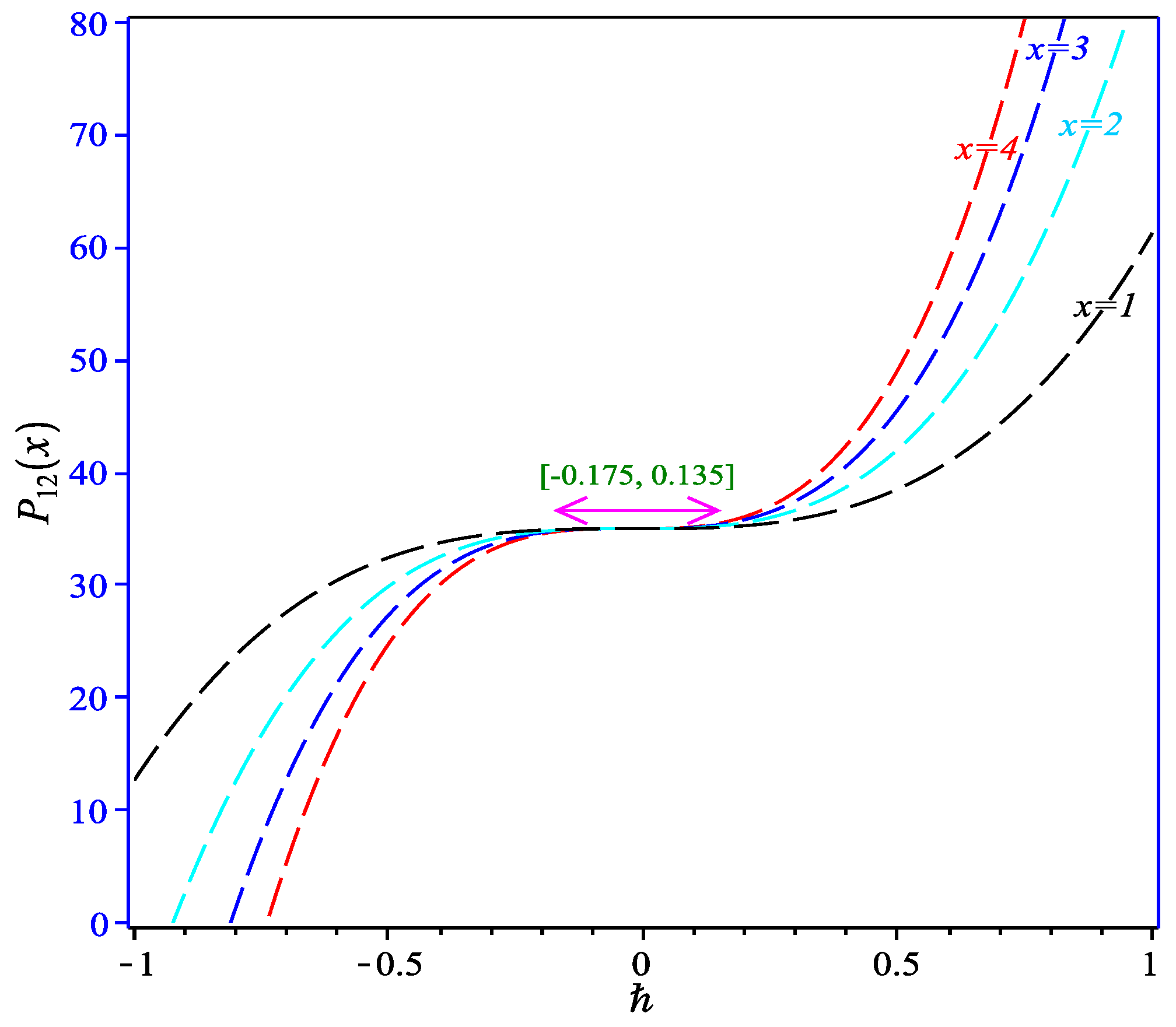
Equation (47) is a approximation solution for pressure P to the problem Equations (25)–(36) in terms of the convergence parameters ℏ and order with . To find the valid region of ℏ, the ℏ-curves given by the 12th-order HAM approximation at different values of x are drawn in Figure 2; this figure shows the interval of ℏ in which the value of is constant at certain x, and M; we chose the horizontal line parallel to x-axis (ℏ) as a valid region which provides us with a simple way to adjust and control the convergence region.
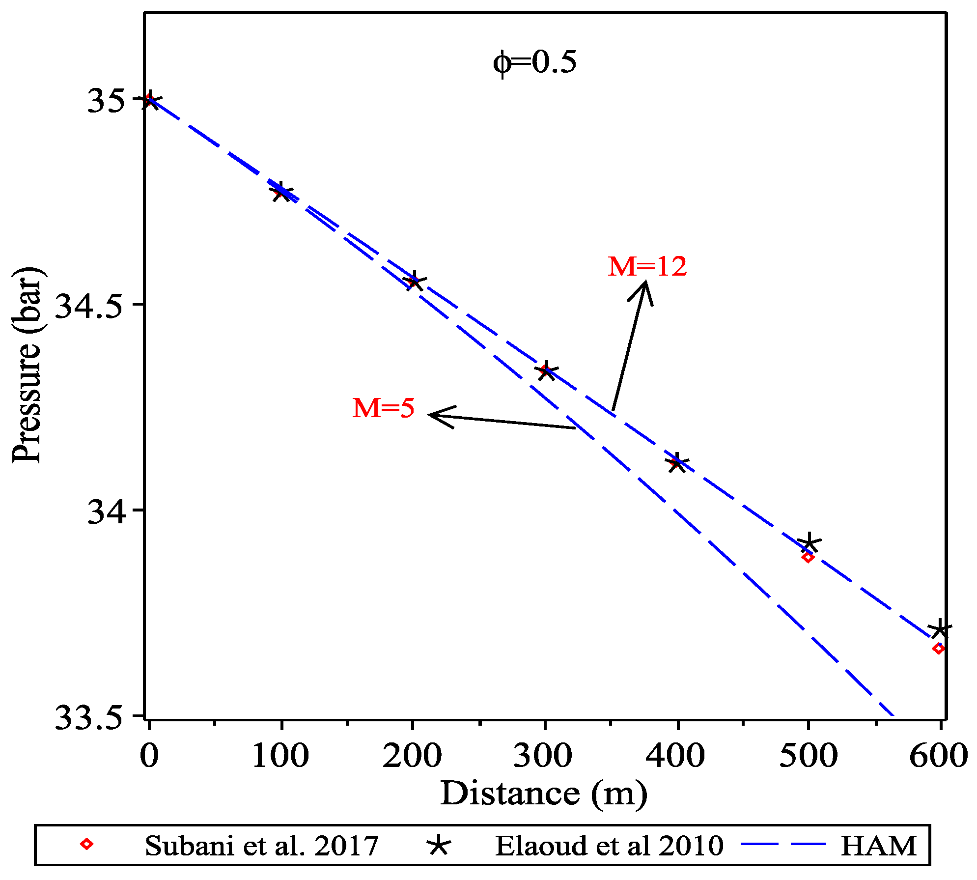
Figure 3 is showing the comparison between the homotopy analysis method with Subani et al., 2017 and Elaoud et al., 2010 methods. In this comparison the order of homotopy analysis method have been used as and . The auxiliary parameter ℏ is chosen as from the convergence interval as showed in the Figure 2. As seen from this figure, with order the homotopy analysis method is comparable with Subani et al., 2017 and Elaoud et al., 2010 methods. In this problem the auxiliary parameter is chosen equal 1.
Now we want to solve the Equations (1) and (2) with the homotopy analysis method (Equations (37)–(46)) using the following initial approximations,
we guessed the initial approximations Equations (48) and (49) using the initial and boundary conditions (for results will be as Equations (3) and (4)). Therefore, using the homotopy analysis method for solving the Equations (1) and (2) with the initial approximation Equations (48) and (49) can obtain the following results,
therefore, pressure is as follows,
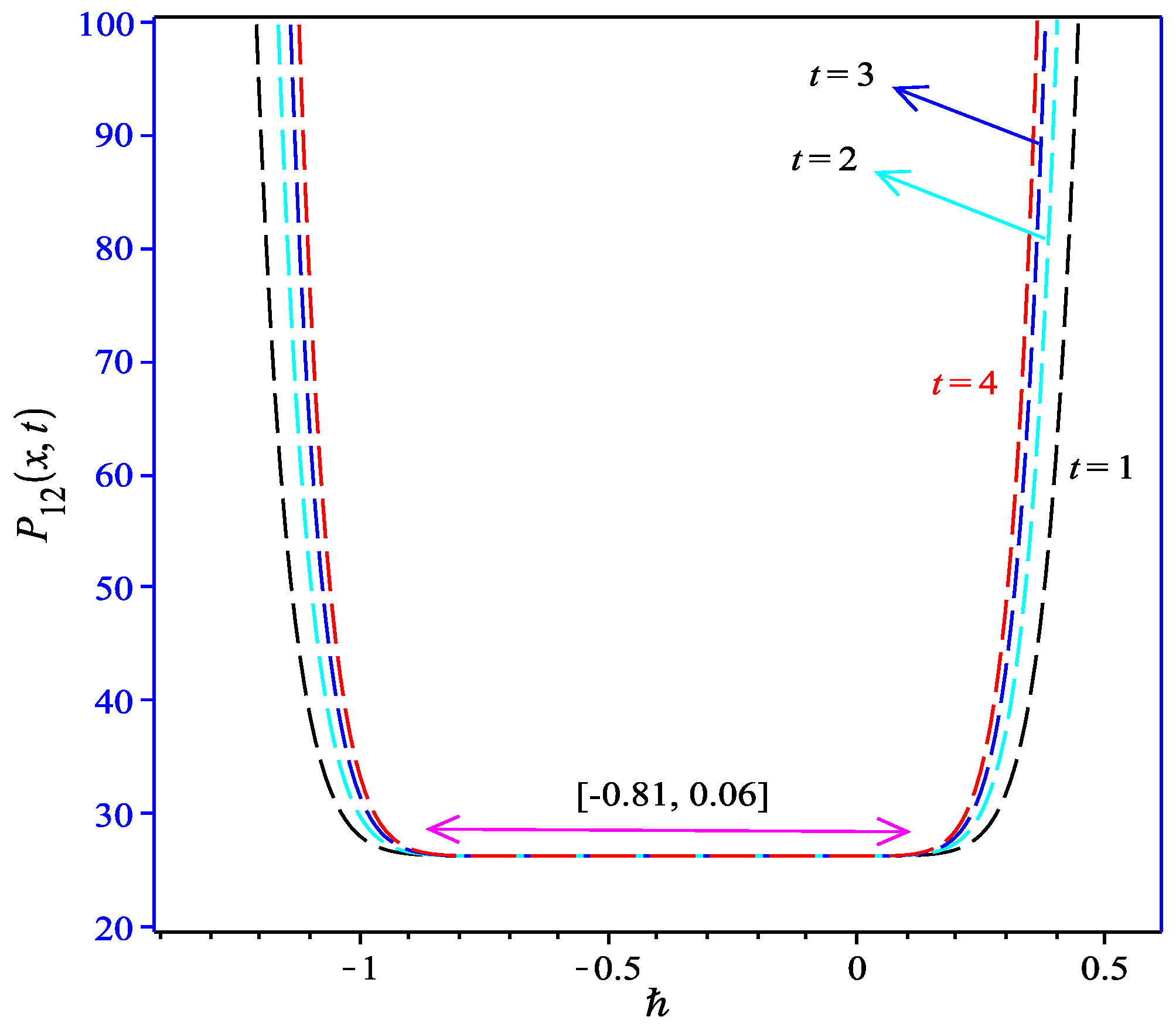
Equation (50) is a approximation solution for pressure to the problem Equations (1) and (2) in terms of the convergence parameters ℏ with . To find the valid region of ℏ, the ℏ-curves given by the 12th-order HAM approximation at different values of t and are drawn in Figure 4; this figure shows the interval of ℏ in which the value of is constant at certain t, and M; we chose the horizontal line parallel to t-axis (ℏ) as a valid region which provides us with a simple way to adjust and control the convergence region.
3.4. Leak Detection Using Homotopy Analysis Method
Because of a small orifice between the high-pressure pipeline and the environment, the orifice of leak can be simulated leaning on the flow rate. The discharged flow from the orifice can be computed by the following Equation [7],
where is the leak orifice area with radius , is the pressure of gas mixture at the leak position and is the density of gas mixture at the leak position respectively, is a discharge coefficient and is the distance of leak from the reservoir.
Analyzing transient pressure wave for hydrogen/natural gas mixtures is based on transmission and reflection properties of pressure wave effected by a downstream valves sudden closure. When the initial pressure wave reaches the leak, it will produce a reflection as it arrives back at the downstream end section. Then, the difference in time between the initial transient wave and the reflected wave is measured and the leakage position in the pipeline is computed by,
where is defined as the distance between the leak and upstream end section, is the difference of time between the initial transient wave and reflected wave and is defined as the transient celerity wave at time.
3.5. Results and Discussion
Figure 5 presents the transient pressure of hydrogen natural gas mixture for isothermal flow when leakage occurs at in horizontal pipeline. The homotopy analysis method of order with has been used. This figure shows the comparison between homotopy analysis method from order 12 and Subani et al. method [7] when and .
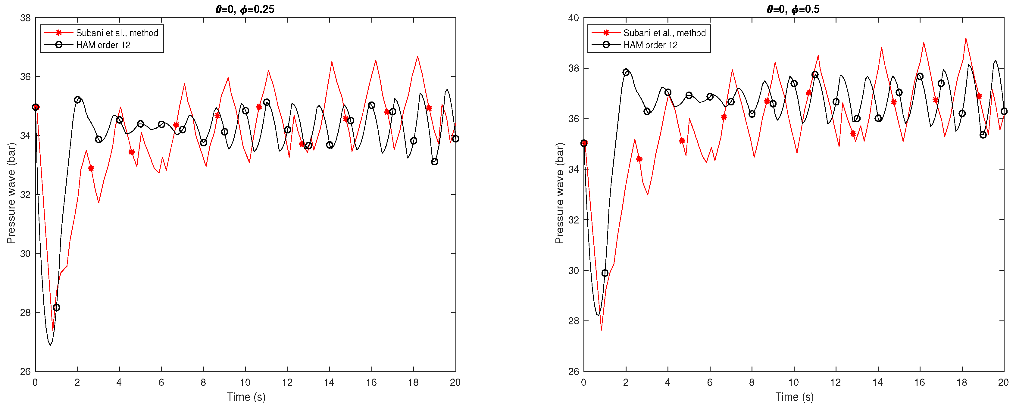
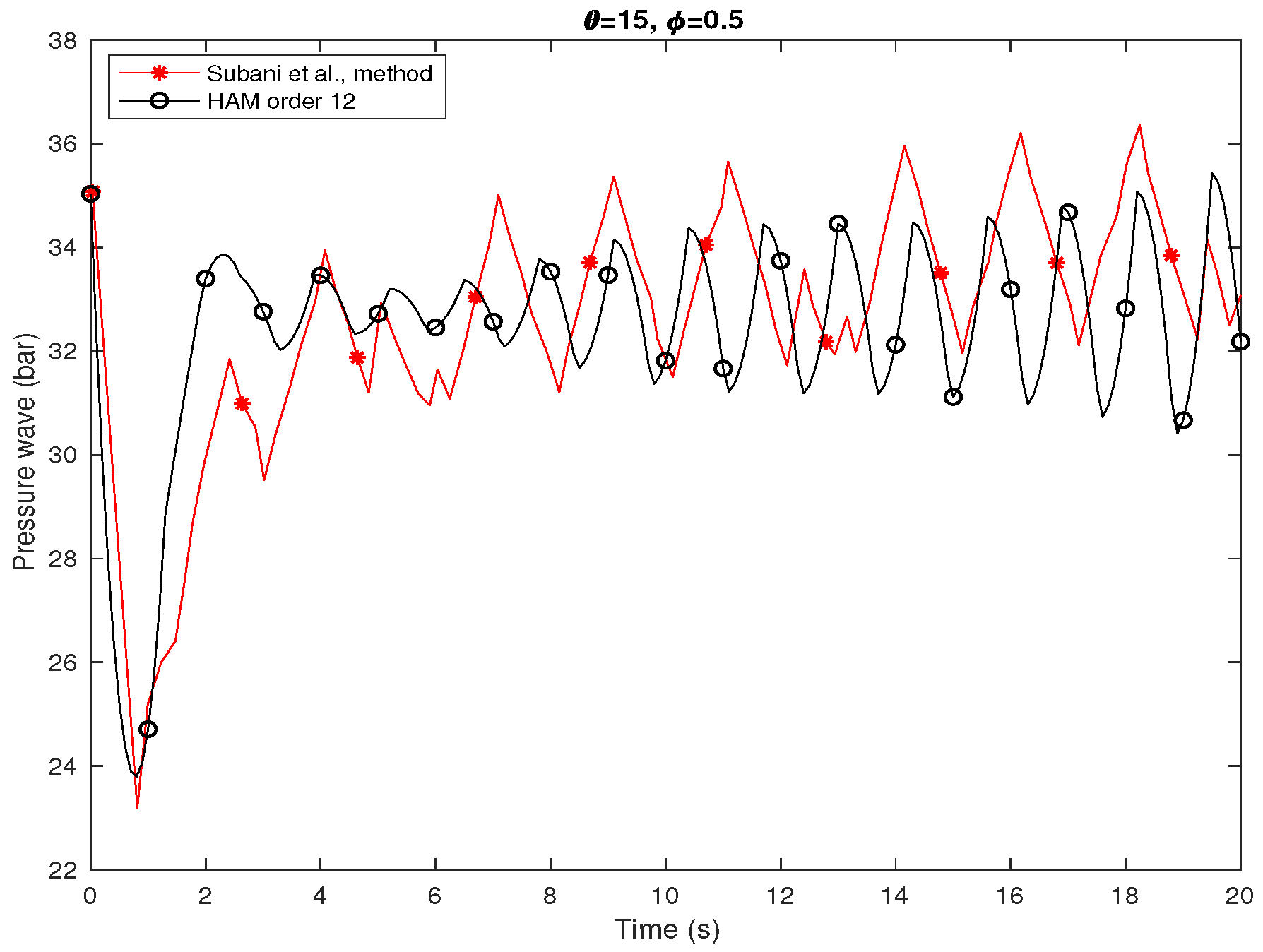
Figure 6 shows the transient pressure of hydrogen natural gas mixture () for isothermal flow when leakage occurs at in an inclined pipeline with . Black line is homotopy analysis method from order 12 with and red line is Subani et al. method. As indicated in Figure 5 and Figure 6, the leak point are estimated at and at for Subani et al. method and HAM respectively.
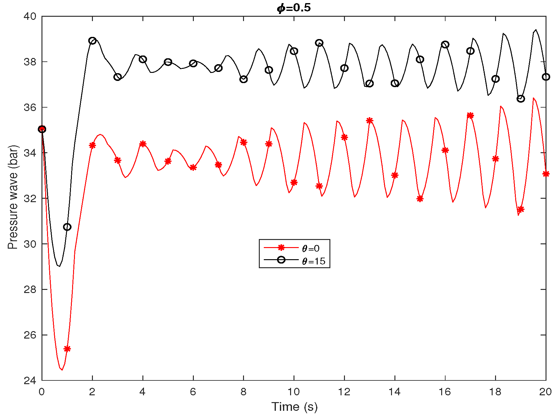
The transient pressure of mixture of natural gas and hydrogen with a mass ratio of is shown in Figure 7 in case of isothermal flow and leak location at with diverse angles. The homotopy analysis method from order 12 and has been used. Red line is for and black line is for .
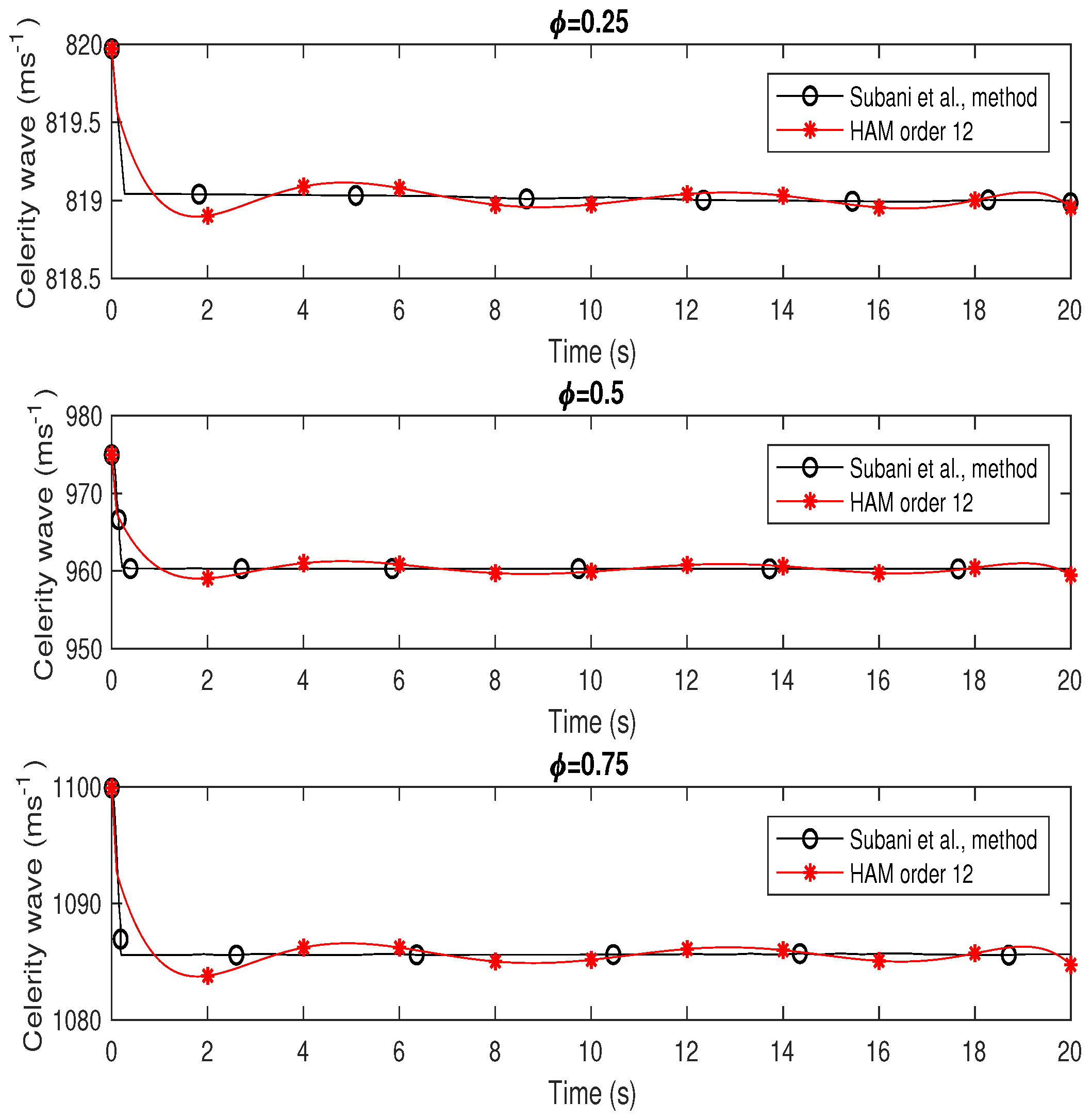
The celerity wave distribution is presented in Figure 8 as a function of time. In this case, the valve of the horizontal pipeline containing different mass ratios of a mixture of gas and hydrogen is abruptly closed when the leakage is at . The values of celerity wave of the leak point for various mass rations are 819.20 ms, 964.60 ms and 1086.60 ms for and , respectively.
As shown in Figure 6 and Figure 7, the occurrence of the leakage is possible when is equal to s. Equation (53) can be used to calculate the leak location of the mixture of natural gas and hydrogen in case of an isothermal flow in a horizontal pipeline as follows:
As seen earlier, there are various mass ratios of the mixture and various angles of the pipeline each with a specific leak location at , the values of which are presented in Table 3. It can be inferred that the leak location is not a function of pipe angle, it is rather a function of the mass ratio of the natural gas and hydrogen mixture. Therefore, mass ratio is of utmost importance here.
The real location of leak is 200 m, when the leak location is at . The leak location calculations by Subani et al. and HAM turned out to be m and m, respectively. It is a mixture of natural gas and hydrogen with a mass ratio of . When the mass ration is increased to , the leakage location is less than 200 m. Therefore, when the mass ratio is decreased, the location is greater than 200 m. This is contrary to the calculations since the calculated value is less than 200 m when the mass ratio is . This is an indication of the dependence of leak location of mass ratio of the mixture considered. As Elaoud et al., (2010) state, the most important part in early determination of a leak close to the reservoir or compressor is the bottom of the pipeline.
Figure 9 shows the leak location with respect to the gas mixture (). As can be seen from this figure, there is a steep slope for the values and , but for values there is a mild slope.
In real (physical) pipelines, noise is expected to affect measurements [35,36]. The possible effects of noisy signals on the performance of the proposed method are Brownian motion or Wiener process or White noise, as the physical model of the stochastic procedure, as an indexed collection random variables. A Wiener process (notation ) is named in the honor of Prof. Norbert Wiener; other name is the Brownian motion (notation ). Wiener process is Gaussian process. As any Gaussian process, Wiener process is completely described by its expectation and correlation functions. A Brownian motion, also called a Wiener process, is obtained as the integral of a white noise signal as follows,
The effects of noisy signals on the effectiveness of the proposed method and possible effects of noisy signals on the performance of leak locations will be proposed in the future works, by introducing white noise in the simulations.
For accurate pinpointing, we can use the zero-gradient control (ZGC) method which we have discussed in our recently published paper [6] about optimal mixture and controlling the pressure. In our next manuscript with title “Detecting Optimal Leak Locations using Delta Method and Zero Gradient Control for Non-isothermal Hydrogen/Natural Gas Mixture in an Inclined Pipeline” we used the delta method (DM) and zero gradient control (ZGC) method for detecting optimal leak locations. In our future works we will mixed the proposed methods with Artificial intelligence, Neural Network and Deep Learning [37] to predict and estimate the optimal mixture parameter for achieving more accurate pinpointing.
4. Conclusions
The homotopy analysis method used to solve the flow equations of hydrogen natural gas mixture in an inclined pipeline. To validate the approximation series for pressure compared with the Subani et al. method. The results in Figure 3, Figure 5 and Figure 6 show that the obtained results using proposed method are in good agreement with the reduced order modelling (ROM) proposed by Subani et al, in 2017. Then, homotopy analysis method is working as well as other methods and give the semi-analytical solutions.
The leak locations were detected using the homotopy analysis method for horizontal pipeline () and inclined pipeline () for gas mixture . Using the homotopy analysis method the celerity wave at leak point of the pipeline are 819.20 ms, 964.60 ms and 1086.60 ms for and , respectively.
In an inclined pipeline the leak location for gas mixture using the Subani et al. method (ROM) and homotopy analysis method respectively are 211.1 m and 210.3 m. Because of the real leak location is supposed at when the leak is located at , the result of HAM method is more accurate than ROM method. As can be seen from Figure 9, with increases the gas mixture from 0 to 1 the leak location decreases and there is a steep slope for , and a mild slope for .
The proposed HAM method is employed without using linearization, discretization, or transformation. It may be concluded that the HAM is very powerful and efficient in finding the analytical solutions for a wide class of gas transportation equations in a pipeline.
Author Contributions
Funding acquisition: N.A. and Z.I.; Methodology: S.S.C.; Software: S.S.C.; Supervision: N.A.; Writing (original draft): S.S.C.; Writing (review and editing): N.A. and Z.I. All authors have read and agreed to the published version of the manuscript.
Funding
This research received no external funding.
Acknowledgments
The authors gratefully acknowledge financial support from the Ministry of Higher Education, Malaysia and Universiti Teknologi Malaysia through Research and Innovation University Grant Scheme, UTMFR Grant (Vot No. Q.J130000.2554.21H48 and FRGS Grant (Vot No R.J130000.7854.5F255).
Conflicts of Interest
The authors declare that there was no conflict of interest regarding the publication of this paper.
References
- Elaoud, S.; Hadj-Taieb, E. Transient flow in pipelines of high-pressure hydrogen-natural gas mixtures. Int. J. Hydrog. Energy 2008, 33, 4824–4832. [Google Scholar] [CrossRef]
- Chaczykowski, M. Transient flow in natural gas pipeline the effect of pipeline thermal model. Appl. Math. Model. 2010, 34, 1051–1067. [Google Scholar] [CrossRef]
- Karney, B.W.; Ruus, E. Charts for water hammer in pipelines resulting from valve closure from full opening only. Can. Civ. Eng. 1985, 12, 241–264. [Google Scholar] [CrossRef]
- Kim, H.; Kim, S.; Kim, Y.; Kim, J. Optimization of Operation Parameters for Direct Spring Loaded Pressure Relief Valve in a Pipeline System. J. Press. Vessel Technol. 2018, 140, 051603. [Google Scholar] [CrossRef]
- Jalving, J.; Zavala, V.M. An Optimization-Based State Estimation Framework for Large-Scale Natural Gas Networks. Ind. Eng. Chem. Res. 2018, 57, 5966–5979. [Google Scholar] [CrossRef]
- Seddighi Chahrborj, S.; Amin, N. Controlling the pressure of hydrogen-natural gas mixture in an inclined pipeline. PLoS ONE 2020, 15, e0228955. [Google Scholar]
- Subani, N.; Amin, N.; Agaie, B.G. Leak detection of non-isothermal transient flow of hydrogennatural gas mixture. J. Loss Prev. Process. Ind. 2017, 48, 244–253. [Google Scholar] [CrossRef]
- Subani, N.; Amin, N. Analysis of water hammer with different closing valve laws on transient flow of hydrogen-natural gas mixture. Abstr. Appl. Anal. 2015, 2015, 1–12. [Google Scholar] [CrossRef] [Green Version]
- Subani, N.; Amin, N.; Agaie, B.G. Hydrogen-natural gas mixture leak detection using reduced order modelling. Appl. Comput. Math. 2015, 4, 135–144. [Google Scholar] [CrossRef]
- Uilhoorn, F.E. Dynamic behaviour of non-isothermal compressible natural gases mixed with hydrogen in pipelines. Int. J. Hydrog. Energy 2009, 34, 6722–6729. [Google Scholar] [CrossRef]
- Veziroglu, T.N.; Barbir, F. Hydrogen: The wonder fuel. Int. J. Hydrog. Energy 1992, 17, 391–404. [Google Scholar] [CrossRef]
- Ebrahimzadeh, E.; Shahrak, M.N.; Bazooyar, B. Simulation of transient gas flow using the orthogonal collocation method. Chem. Eng. Res. Des. 2012, 90, 1701–1710. [Google Scholar] [CrossRef]
- Elaoud, S.; Hadj-Taieb, E. Leak detection of hydrogen-natural gas mixtures in pipes using the pressure-time transient analysis. In Proceedings of the Conference and Exposition International of Ecologic Vehicles and Renewable Energy (EVRE), Monte Carlo, Monaco, 2019. [Google Scholar]
- Elaoud, S.; Hadj-Taeb, L.; Hadj-Taeb, E. Leak detection of hydrogennatural gas mixtures in pipes using the characteristics method of specified time intervals. J. Loss Prev. Process. Ind. 2010, 23, 637–645. [Google Scholar] [CrossRef]
- Turner, W.J.; Mudford, N.R. Leak detection, timing, location and sizing in gas pipelines. Math. Comput. Model. 1988, 10, 609–627. [Google Scholar] [CrossRef]
- Wilkening, H.; Baraldi, D.C.F.D. CFD modelling of accidental hydrogen release from pipelines. Int. J. Hydrog. Energy 2007, 32, 2206–2215. [Google Scholar] [CrossRef]
- Puust, R.; Kapelan, Z.; Savic, D.A.; Koppel, T. A review of methods for leakage management in pipe networks. Urban Water J. 2010, 7, 25–45. [Google Scholar] [CrossRef]
- Diao, X.; Shen, G.; Jiang, J.; Chen, Q.; Wang, Z.; Ni, L.; Mebarki, A.; Dou, Z. Leak detection and location in liquid pipelines by analyzing the first transient pressure wave with unsteady friction. J. Loss Prev. Process. Ind. 2019, 60, 303–310. [Google Scholar] [CrossRef]
- Li, S.; Zhang, J.; Yan, D.; Wang, P.; Huang, Q.; Zhao, X.; Cheng, Y.; Zhou, Q.; Xiang, N.; Dong, T. Leak detection and location in gas pipelines by extraction of cross spectrum of single non-dispersive guided wave modes. J. Loss Prev. Process. Ind. 2016, 44, 255–262. [Google Scholar] [CrossRef]
- Silva, R.A.; Buiatti, C.M.; Cruz, S.L.; Pereira, J.A. Pressure wave behaviour and leak detection in pipelines. Comput. Chem. Eng. 1996, 20, S491–S496. [Google Scholar] [CrossRef]
- Ge, C.; Wang, G.; Ye, H. Analysis of the smallest detectable leakage flow rate of negative pressure wave-based leak detection systems for liquid pipelines. Comput. Chem. 2008, 32, 1669–1680. [Google Scholar] [CrossRef]
- Brunone, B.; Ferrante, M. Detecting leaks in pressurised pipes by means of transients. J. Hydraul. Res. 2001, 39, 539–547. [Google Scholar] [CrossRef]
- Martini, A.; Rivola, A.; Troncossi, M. Autocorrelation analysis of vibro-acoustic signals measured in a test field for water leak detection. Appl. Sci. 2018, 8, 2450. [Google Scholar] [CrossRef] [Green Version]
- Brennan, M.J.; Gao, Y.; Ayala, P.C.; Almeida, F.C.L.; Joseph, P.F.; Paschoalini, A.T. Amplitude distortion of measured leak noise signals caused by instrumentation: Effects on leak detection in water pipes using the cross-correlation method. J. Sound Vib. 2019, 461, 114905. [Google Scholar] [CrossRef]
- Martini, A.; Troncossi, M.; Rivola, A. Leak detection in water-filled small-diameter polyethylene pipes by means of acoustic emission measurements. Appl. Sci. 2017, 7, 2. [Google Scholar] [CrossRef] [Green Version]
- Liu, C.; Li, Y.; Fang, L.; Xu, M. New leak-localization approaches for gas pipelines using acoustic waves. Measurement 2019, 134, 54–65. [Google Scholar] [CrossRef]
- Li, J.; Zheng, Q.; Qian, Z.; Yang, X. A novel location algorithm for pipeline leakage based on the attenuation of negative pressure wave. Process Saf. Environ. 2019, 123, 309–316. [Google Scholar] [CrossRef]
- Liao, S.J. The Proposed Homotopy Analysis Technique for the Solution of Nonlinear Problems. Ph.D. Thesis, Shanghai Jiao Tong University, Shanghai, China, 1992. [Google Scholar]
- Rana, P.; Shukla, N.; Gupta, Y.; Pop, I. Homotopy analysis method for predicting multiple solutions in the channel flow with stability analysis. Commun. Nonlinear Sci. Numer. Simul. 2019, 66, 183–193. [Google Scholar] [CrossRef]
- Yu, C.; Wang, H.; Fang, D.; Ma, J.; Cai, X.; Yu, X. Semi-analytical solution to one-dimensional advective-dispersive-reactive transport equation using homotopy analysis method. J. Hydrol. 2018, 565, 422–428. [Google Scholar] [CrossRef]
- Seddighi Chahrborj, S.; Sadat Kiai, S.M.; Abu Bakar, M.R.; Ziaeian, I.; Gheisari, Y. Homotopy analysis method to study a quadrupole mass filter. J. Mass Spectrom. 2012, 47, 484–489. [Google Scholar] [CrossRef]
- Seddighi Chahrborj, S.; Moameni, A. Spectral-homotopy analysis of MHD non-orthogonal stagnation point flow of a nanofluid. J. Appl. Math. Comput. Mech. 2018, 17. [Google Scholar] [CrossRef] [Green Version]
- Liao, S. Beyond Perturbation: Introduction to the Homotopy Analysis Method; CRC Press: Boca Raton, FL, USA, 2003. [Google Scholar]
- Mehmood, A.; Munawar, S.; Ali, A. Comments to: Homotopy analysis method for solving the MHD flow over a non-linear stretching sheet (Commun. Nonlinear Sci. Numer. Simul. 14 (2009) 26532663). Commun. Nonlinear Sci. Numer. 2010, 15, 4233–4240. [Google Scholar] [CrossRef]
- Mandal, P.C. Gas leak detection in pipelines & repairing system of titas gas. J. Appl. Eng. 2014, 2, 23–34. [Google Scholar]
- Seddighi Chahrborj, S.; Kiai, S.M.S.; Arifina, N.M.; Gheisari, Y. Applications of Stochastic Process in the Quadrupole Ion traps. Mass Spectrom. Lett. 2015, 6, 91–98. [Google Scholar] [CrossRef]
- Seddighi Chahrborj, S.; Chaharborj, S.S.; Mahmoudi, Y. Study of fractional order integro-differential equations by using Chebyshev Neural Network. J. Math. Stat. 2017, 13, 1–13. [Google Scholar] [CrossRef]
Publisher’s Note: MDPI stays neutral with regard to jurisdictional claims in published maps and institutional affiliations. |
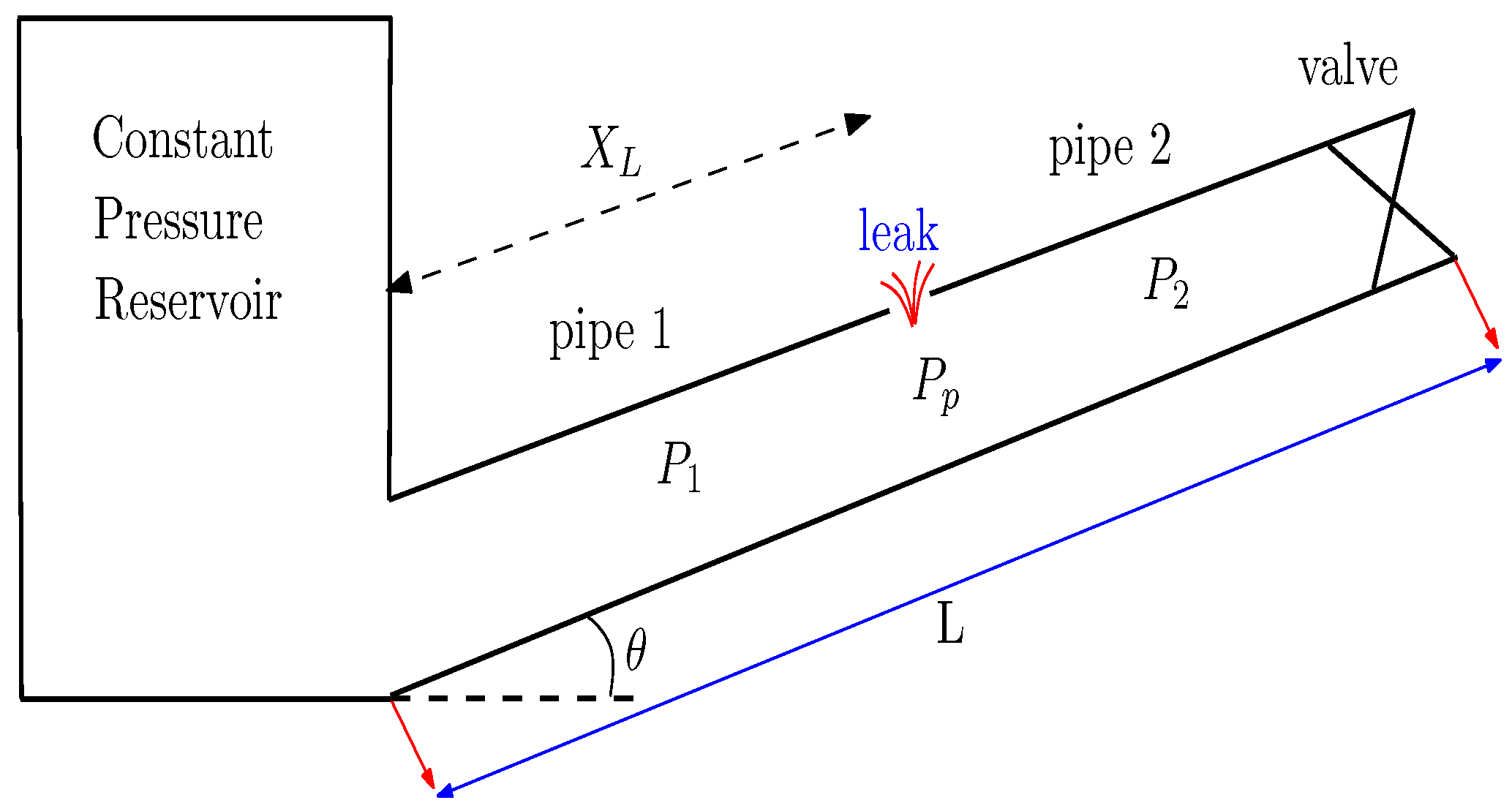
Figure 1.
An inclined pipeline with a reservoir at the top and a valve at its bottom.

Figure 2.
ℏ-curve for HAM approximation solution of the problem Equations (5) and (6) at different values of x.

Figure 3.
Comparison between homotopy analysis method of orders for ; with Subani et al., 2017 and Elaoud et al., 2010 methods.
Figure 3.
Comparison between homotopy analysis method of orders for ; with Subani et al., 2017 and Elaoud et al., 2010 methods.

Figure 4.
ℏ-curve for HAM approximation solution of the problem Equations (1) and (2) at different values of t and .

Figure 5.
Transient pressure of hydrogen natural gas mixture for isothermal flow when leakage occurs at in horizontal pipeline when and .
Figure 5.
Transient pressure of hydrogen natural gas mixture for isothermal flow when leakage occurs at in horizontal pipeline when and .

Figure 6.
Transient pressure of hydrogen natural gas mixture for isothermal flow when leakage occurs at in an inclined pipeline when and .
Figure 6.
Transient pressure of hydrogen natural gas mixture for isothermal flow when leakage occurs at in an inclined pipeline when and .

Figure 7.
Transient pressure of hydrogen natural gas mixture with for isothermal flow when leakage occurs at with different angles . HAM with order 12 and .
Figure 7.
Transient pressure of hydrogen natural gas mixture with for isothermal flow when leakage occurs at with different angles . HAM with order 12 and .

Figure 8.
Celerity wave of hydrogen natural gas mixture for isothermal flow when leakage occurs at in horizontal pipeline with different mass ratio .
Figure 8.
Celerity wave of hydrogen natural gas mixture for isothermal flow when leakage occurs at in horizontal pipeline with different mass ratio .

Figure 9.
Leak location with respect to the gas mixture ().


Table 1.
Hydrogen properties in working conditions, bar and C = 288 K (See [7]).
Table 1.
Hydrogen properties in working conditions, bar and C = 288 K (See [7]).
| Symbol | Fluid Properties | Values (J/kgK) | |
|---|---|---|---|
| Hydrogen | Natural Gas | ||
| Specific heat at constant pressure | 14,600 | 1497.5 | |
| Specific heat at constant volume | 10,440 | 1056.8 | |
| R | Gas constant | 4160 | 440.7 |
Table 2.
Parameters used for the simulation (See [7]).
Table 2.
Parameters used for the simulation (See [7]).
| Symbols | Values | Symbols | Values |
|---|---|---|---|
| Pipe length | L = 600 m | Mass ratio | |
| Time | t = 20 | Angle | |
| Pipe diameter | D = m | Mass flow | = 55 kg/s |
| Friction coefficient | Absolute pressure | = 35 bar | |
| Temperature | C = 288 K |
Table 3.
Leak location for the hydrogen-natural gas mixture for isothermal flow at leakage .
| Gas Mixture | Pipeline’s Angle | Leak Location (m) | |
|---|---|---|---|
| Subani et al., Method | HAM | ||
| 0 | 439.4 | 439.8 | |
| 439.4 | 439.8 | ||
| 0.25 | 268.3 | 269.04 | |
| 268.3 | 269.04 | ||
| 0.5 | 211.1 | 210.3 | |
| 211.1 | 210.3 | ||
| 0.75 | 160.6 | 161.01 | |
| 160.6 | 161.01 | ||
| 1 | 95.8 | 96.2 | |
| 95.8 | 96.2 | ||
© 2020 by the authors. Licensee MDPI, Basel, Switzerland. This article is an open access article distributed under the terms and conditions of the Creative Commons Attribution (CC BY) license (http://creativecommons.org/licenses/by/4.0/).
Share and Cite
MDPI and ACS Style
S. Chaharborj, S.; Ismail, Z.; Amin, N. Detecting Optimal Leak Locations Using Homotopy Analysis Method for Isothermal Hydrogen-Natural Gas Mixture in an Inclined Pipeline. Symmetry 2020, 12, 1769. https://doi.org/10.3390/sym12111769
AMA Style
S. Chaharborj S, Ismail Z, Amin N. Detecting Optimal Leak Locations Using Homotopy Analysis Method for Isothermal Hydrogen-Natural Gas Mixture in an Inclined Pipeline. Symmetry. 2020; 12(11):1769. https://doi.org/10.3390/sym12111769
Chicago/Turabian StyleS. Chaharborj, Sarkhosh, Zuhaila Ismail, and Norsarahaida Amin. 2020. "Detecting Optimal Leak Locations Using Homotopy Analysis Method for Isothermal Hydrogen-Natural Gas Mixture in an Inclined Pipeline" Symmetry 12, no. 11: 1769. https://doi.org/10.3390/sym12111769
Note that from the first issue of 2016, this journal uses article numbers instead of page numbers. See further details here.